SUSX-TH-98-001
SUSSEX-AST 98/2-4
FERMILAB-Pub-97/434-A
astro-ph/9802209

On the reliability of inflaton
potential reconstruction

Edmund J. Copeland

Centre for Theoretical Physics, University of Sussex
Falmer, Brighton BN1 9QH, United Kingdom

Ian J. Grivell

Astronomy Centre, University of Sussex
Falmer, Brighton BN1 9QJ, United Kingdom

Edward W. Kolb

NASA/Fermilab Astrophysics Center, Fermi National Accelerator Laboratory
Batavia, Illinois 60510
and
Department of Astronomy and Astrophysics and Enrico Fermi Institute
The University of Chicago, Chicago, Illinois 60637

Andrew R. Liddle

Astronomy Centre, University of Sussex
Falmer, Brighton BN1 9QJ, United Kingdom

If primordial scalar and tensor perturbation spectra can be inferred from observations of the cosmic background radiation and large-scale structure, then one might hope to reconstruct a unique single-field inflaton potential capable of generating the observed spectra. In this paper we examine conditions under which such a potential can be reliably reconstructed. For it to be possible at all, the spectra must be well fit by a Taylor series expansion. A complete reconstruction requires a statistically-significant tensor mode to be measured in the microwave background. We find that the observational uncertainties dominate the theoretical error from use of the slow-roll approximation, and conclude that the reconstruction procedure will never insidiously lead to an irrelevant potential.

PACS numbers: 98.70.Vc, 98.80.Cq

1 Inflation and Perturbations

Inflation produces metric perturbations, which are presently the most plausible cause of the observed temperature fluctuations in the cosmic background radiation (CBR) and which may act as the seeds for structure formation. During inflation the Hubble radius $H^{-1}$ ($H=\dot{a}/a$ is the expansion rate) must have increased more slowly than the scale factor $a$, while during the radiation and matter eras it increased as $a^{2}$ and $a^{3/2}$, respectively. The dynamics of the evolution of the Hubble radius (or, equivalently, the evolution of the expansion rate $H$) during inflation is usually modelled by assuming that the energy density is dominated by scalar-field potential energy. The number of dynamical degrees of freedom associated with the evolution of the scalar-field potential energy (and hence the Hubble radius) is unknown. If there is only one relevant degree of freedom, that degree of freedom is called the inflaton, and the scalar-field potential is called the inflaton potential.

Inflation models where a single inflaton field slowly evolves under the influence of the inflaton potential are called single-field slow-roll models. Such models are very attractive because of their simplicity, because they arise naturally in a host of particle physics models, and because other more complicated models can often be expressed in terms of an effective single-field slow-roll model.

The assumption that only a single scalar field is dynamically relevant can, at least in principle, be tested by a series of consistency relations which represent relations between the scalar and tensor perturbations produced in single-field models [1, 2]. Inflation models where more than one scalar field is dynamically important are phenomenologically much more complicated, and almost certainly must be studied on a case-by-case basis. In this paper we shall restrict our discussion to the single-field case, where the scalar potential $V(\phi)$ is the only piece of information to be specified.

Reconstruction of the inflaton potential (see Ref. [2] for a review) refers to the process of using observational data, especially microwave background anisotropies, to determine the inflaton potential capable of generating the perturbation spectra inferred from observations [1]. Of course there is no way to prove that the reconstructed inflaton potential was the agent responsible for generating the perturbations. What can be hoped for is that one can determine a unique (within observational errors) inflaton potential capable of producing the observed perturbation spectra. The reconstructed inflaton potential may well be the first concrete piece of information to be obtained about physics at scales close to the Planck scale.

As is well known, inflation produces both scalar and tensor perturbations, which each generate microwave anisotropies (see Ref. [3] for a review). As reviewed in the next section, if $V(\phi)$ is given the perturbation spectra can be computed exactly in linear perturbation theory through integration of the relevant mode equations. If the scalar field is rolling sufficiently slowly, the solutions to the mode equations may be approximated using the slow-roll expansion [4, 5, 6]. The standard reconstruction program makes use of the slow-roll expansion, taking advantage of a calculation of the perturbation spectra by Stewart and Lyth [7], which gives the next-order correction to the usual lowest-order slow-roll results.

The biggest hurdle for successful reconstruction is that many inflation models predict a tensor perturbation amplitude well below the expected threshold for detection, and as we will see, even above detection threshold the errors can be considerable. If the tensor modes cannot be identified a unique reconstruction is impossible, as the scalar perturbations are governed not only by $V(\phi)$, but by the first derivative of $V(\phi)$ as well. Knowledge of only the scalar perturbations leaves an undetermined integration constant in the non-linear system of reconstruction equations. Another problem is that simple potentials usually lead to a nearly exact power-law scalar spectrum with the spectral index close to unity. In such a scenario only a very limited amount of information could be obtained about high energy physics from astrophysical observations.

Recently, Wang et al. [8] suggested an alternative danger to reconstruction. They studied the possibility that the potential might be sufficiently complicated that the slow-roll expansion breaks down, and a full integration of the mode functions is necessary to calculate the perturbation spectra to the accuracy expected by the next round of satellite observations by map and Planck.

It is, of course, clear that any perturbative procedure such as the slow-roll expansion has some limit to its validity. But here, the breakdown of the slow-roll expansion is particularly troublesome; firstly because of the technical difficulty that there is no known method of computing yet higher-order corrections, and secondly because there is a general possibility that for sufficiently complicated potentials the perturbation series may not converge at all. However, the key concern for reconstruction is whether such a situation will lead to a misconstruction of the inflaton potential.

In this paper, we shall argue that for the purpose of reconstruction the breakdown of the slow-roll approximation is in many senses desirable. First of all, we show that there is no practical danger that one can be misled into thinking perturbative reconstruction is working when in fact it is not. Secondly, the very failure of the perturbative approach implies that extra parameters are required in order to explain the observed data set, and hence there is the prospect of obtaining a greater amount of information about the inflationary model. Finally, we will demonstrate that the theoretical errors from the use of slow-roll equations are sub-dominant to the expected observational errors from a satellite experiment such as Planck.

Wang et al. [8] described a particular, admittedly rather ad hoc, scalar field potential, for which they demonstrated that the result of exact mode equation integration differed significantly, by the standards of say the Planck satellite, from the slow-roll expansion. We shall largely concentrate on that potential as a means of concrete illustration of the very general points we shall make.

2 The slow-roll expansion

Two crucial ingredients for reconstruction are the primordial scalar and tensor perturbation spectra $A_{S}(k)$ and $A_{T}(k)$ which we define as in Ref. [2]. We define slow-roll parameters $\epsilon$, $\eta$, and $\xi$ as

$$\epsilon(\phi) \equiv \frac{m_{{\rm Pl}}^{2}}{4\pi}\left[\frac{H^{\prime}(\phi)}{H(\phi)}\right]^{2}$$ (2.1)

$$\eta(\phi) \equiv \frac{m_{{\rm Pl}}^{2}}{4\pi}\frac{H^{\prime\prime}(\phi)}{H(\phi)}$$ (2.2)

$$\xi(\phi) \equiv \frac{m_{{\rm Pl}}^{2}}{4\pi}\left(\frac{H^{\prime}(\phi)H^{\prime\prime\prime}(\phi)}{H^{2}(\phi)}\right)^{1/2}\ ,$$ (2.3)

where here and throughout the paper the prime superscript implies $d/d\phi$. As long as these parameters are small compared to unity, $A_{S}(k)$ and $A_{T}(k)$ are given by [7]

$$A_{S}^{2}(k) \simeq \frac{4}{25\pi}\left(\frac{H}{m_{{\rm Pl}}}\right)^{2}\left(\frac{1}{\epsilon}\right)\left[1-(2C+1)\epsilon+C\eta\right]^{2}$$ (2.4)

$$A_{T}^{2}(k) \simeq \frac{4}{25\pi}\left(\frac{H}{m_{{\rm Pl}}}\right)^{2}\left[1-(C+1)\epsilon\right]^{2}\ ,$$ (2.5)

where $H(\phi)$, $\epsilon(\phi)$, and $\eta(\phi)$ are to be determined at the value of $\phi$ when $k=aH$ during inflation, and where $C=-2+\ln 2+\gamma\simeq-0.73$ is a numerical constant, $\gamma$ being the Euler constant. These equations are the basis of the reconstruction process and provide an analytic alternative to integration of the full mode equations.

The expressions for $A^{2}_{S}(k)$ and $A^{2}_{T}(k)$ are in terms of $H(\phi)$ and the slow-roll parameters $\epsilon(\phi)$ and $\eta(\phi)$, but what is usually known is the potential $V(\phi)$. Since $H$ can be written exactly in terms of $V$ and $\epsilon$:

$$\frac{H^{2}(\phi)}{m_{{\rm Pl}}^{2}}=8\pi\,\frac{V(\phi)}{m_{{\rm Pl}}^{4}}\,\frac{1}{3-\epsilon(\phi)}\ ,$$ (2.6)

the problem reduces to finding $\epsilon$ and $\eta$ in terms of $V$ and its derivatives.

There are two methods to determine $H$ and the slow-roll parameters. The first is an analytic approach studied by Kolb and Vadas [9] and by Liddle et al. [6]. (The results are identical; here we follow the notation of the later paper.) The approach involves an infinite hierarchy of potential slow-roll parameters:

$$\epsilon_{\scriptscriptstyle V}(\phi)=\frac{m_{{\rm Pl}}^{2}}{16\pi}\left(\frac{V^{\prime}}{V}\right)^{2}\qquad \qquad\eta_{\scriptscriptstyle V}(\phi)=\frac{m_{{\rm Pl}}^{2}}{8\pi}\,\frac{V^{\prime\prime}}{V}\,,$$ ;

$$\xi^{2}_{{\scriptscriptstyle V}}(\phi)=\frac{m^{2}_{{\rm Pl}}}{8\pi}\,\frac{\left(V^{\prime}\right)^{1}V^{(3)}}{V^{2}}\qquad \qquad\sigma^{3}_{{\scriptscriptstyle V}}(\phi)=\frac{m^{2}_{{\rm Pl}}}{8\pi}\,\frac{\left(V^{\prime}\right)^{2}V^{(4)}}{V^{3}}\,,$$ ; (2.7)

and so on, where $V^{(n)}=d^{n}V/d\phi^{n}$.

The slow-roll parameters of Eqs. (2.1-2.3) involve an infinite number of potential slow-roll parameters, and to obtain an analytic expression it is necessary to truncate the expression by neglecting potential slow-roll parameters above a given order. For most potentials the higher derivatives become small rapidly, and the expressions can be terminated after only a few terms. For instance, to fourth order in $H^{2}$ [6]

$$H^{2}(\phi) = \frac{8\pi}{3m_{{\rm Pl}}^{2}}V(\phi)\left[1+\frac{1}{3}\epsilon_{{\scriptscriptstyle V}}-\frac{1}{3}\epsilon^{2}_{{\scriptscriptstyle V}}++\frac{2}{9}\epsilon_{{\scriptscriptstyle V}}\eta_{{\scriptscriptstyle V}}+\frac{25}{27}\epsilon^{3}_{{\scriptscriptstyle V}}\right.$$ (2.8)

$$+\frac{5}{27}\epsilon_{{\scriptscriptstyle V}}\eta^{2}_{{\scriptscriptstyle V}}-\frac{26}{27}\epsilon^{2}_{{\scriptscriptstyle V}}\eta_{{\scriptscriptstyle V}}+\frac{2}{27}\epsilon_{{\scriptscriptstyle V}}\xi^{2}_{{\scriptscriptstyle V}}-\frac{327}{81}\epsilon^{4}_{{\scriptscriptstyle V}}+\frac{460}{81}\epsilon^{3}_{{\scriptscriptstyle V}}\eta_{{\scriptscriptstyle V}}-\frac{172}{81}\epsilon^{2}_{{\scriptscriptstyle V}}\eta^{2}_{{\scriptscriptstyle V}}$$

$$+\left.\frac{14}{81}\epsilon_{{\scriptscriptstyle V}}\eta^{3}_{{\scriptscriptstyle V}}-\frac{44}{81}\epsilon^{2}_{{\scriptscriptstyle V}}\xi^{2}_{{\scriptscriptstyle V}}+\frac{2}{9}\epsilon_{{\scriptscriptstyle V}}\eta_{{\scriptscriptstyle V}}\xi^{2}_{{\scriptscriptstyle V}}+\frac{2}{81}\epsilon_{{\scriptscriptstyle V}}\sigma^{3}_{{\scriptscriptstyle V}}+\cdots\,\right]$$

and similar expressions can be found in Refs. [6, 9] for $\epsilon(\phi)$, $\eta(\phi)$, etc.

In practice, one would calculate the first few potential slow-roll parameters, and if the ones involving higher derivatives become small, the series may be truncated. However if the higher-derivative slow-roll parameters do not become small, then it is necessary to perform a numerical calculation.

The slow-roll parameters may be calculated numerically quite easily by expressing Eq. (2.6) as an equation for $\epsilon$:

$$\epsilon(\phi)=3-8\pi\frac{V(\phi)}{m^{2}_{{\rm Pl}}H^{2}(\phi)}\ ,$$ (2.9)

taking the derivative with respect to $\phi$, using the expressions for $H^{\prime}$ and $H$ in terms of $\epsilon$ [Eq. (2.1) and Eq. (2.6)] to yield a first-order differential equation satisfied by $\epsilon$,

$$\epsilon^{\prime}=\left(\frac{m_{{\rm Pl}}V^{\prime}}{V}+\sqrt{16\pi\epsilon}\right)(\epsilon-3).$$ (2.10)

It is easy to show that $\eta=\epsilon-m_{{\rm Pl}}\,\epsilon^{\prime}/\sqrt{16\pi\epsilon}$, so using Eq. (2.10) for $\epsilon^{\prime}$ and integrating it to find $\epsilon$, $\eta$ is found. The slow-roll parameter $\xi$ can be expressed in terms of $\epsilon$, $\eta$, and $\eta^{\prime}$ as $\xi^{2}=\epsilon\eta-m_{{\rm Pl}}\eta^{\prime}\sqrt{\epsilon/4\pi}$. For this expression the additional function $\epsilon^{\prime\prime}$ is required, which can be expressed as

$$m^{2}_{{\rm Pl}}\epsilon^{\prime\prime}=\left[\frac{m^{2}_{{\rm Pl}}V^{\prime\prime}}{V}-\left(\frac{m_{{\rm Pl}}V^{\prime}}{V}\right)^{2}+\frac{8\pi m_{{\rm Pl}}\,\epsilon^{\prime}}{\sqrt{16\pi\epsilon}}\right](\epsilon-3)+\left[\frac{m_{{\rm Pl}}V^{\prime}}{V}+\sqrt{16\pi\epsilon}\right].$$ (2.11)

method	$H$; $\epsilon$; $\eta$	$A^{2}_{S}(k)$ and $A^{2}_{T}(k)$
numerical	numerical: Eq. (2.6)	mode equations
semi-analytic	numerical: Eq. (2.6)	slow-roll expressions [Eqs. (2.4) & (2.5)]
higher-order	$H$: Eq. (2.8)
analytic	$\epsilon$: Refs. [6, 9]	slow-roll expressions [Eqs. (2.4) &(2.5)]
	$\eta$: Refs. [6, 9]
lowest-order	$H=8\pi V/3m^{2}_{{\rm Pl}}$	truncation of slow-roll expressions
analytic	$\epsilon=\epsilon_{V}$	[Eqs. (2.4) & (2.5)]
	$\eta=\epsilon_{V}-\eta_{V}$

Table 1: Different approaches to computing the power spectrum from a potential $V(\phi)$.

For the calculation of $A_{S}(k)$ and $A_{T}(k)$ there are three levels of ease/accuracy one may employ as indicated in Table 1. The simplest, but least accurate, method is an analytic approach, using Eq. (2.8) and corresponding ones for $H$, $\epsilon$, and $\eta$, and the slow-roll expressions, Eqs. (2.4) and (2.5), for $A^{2}_{S}(k)$ and $A^{2}_{T}(k)$. This will be accurate if the potential slow-roll parameters $\epsilon_{{\scriptscriptstyle V}}$, $\eta_{{\scriptscriptstyle V}}$, etc. become small, so that a truncation can be performed in the expressions (the analogues of Eq. (2.8)) for the slow-roll parameters $\epsilon$ and $\eta$, and provided the slow-roll parameters are smaller than unity. If $\epsilon$ and $\eta$ are small enough, the square brackets in Eqs. (2.4) and (2.5) may be replaced by unity and the expressions simplify further.

The most accurate and reliable, but most involved, is a numerical calculation in which the slow-roll parameters are calculated numerically and used in a numerical integration of the mode equations.

For some potentials, it may be desirable to perform something we call a semi-analytic calculation, which involves calculating $\epsilon$ and $\eta$ numerically, and using the numerical values in the slow-roll expression for $A^{2}_{S}(k)$ and $A^{2}_{T}(k)$. This will be useful if the higher-order potential slow-roll parameters become large but the actual values of $\epsilon$, $\eta$, and $\xi$ are small. Only one numerical integration is required to compute the spectrum, whereas the mode equation integration must be done for each $k$.

3 The potential

Figure 1: The potential of Eq. 3.1.

Wang et al. [8] consider an inflaton potential of the form

$$V(\phi)=\Lambda^{4}\left(1-\frac{2}{\pi}\,\tan^{-1}\frac{5\phi}{m_{{\rm Pl}}}\right)\,,$$ (3.1)

which is shown in Fig. 1. We shall take $\Lambda=1$; results could be rescaled if desired to match the COBE normalization. With this potential, inflation is everlasting. Wang et al. [8] envisage extra physics, such as a hybrid inflation mechanism [10], intervening to end inflation at some point, and assume that the field’s location at the time observable perturbations were formed can be placed anywhere on the potential. As a specific example, they choose $\phi=-0.3m_{{\rm Pl}}$ to be the value of the field when the present Hubble radius equalled the Hubble radius during inflation. We adopt their choice for the end of inflation.

Fig. 2 shows the potential slow-roll parameters of Eq. (2), $\tau_{{\scriptscriptstyle V}}$ and $\zeta_{{\scriptscriptstyle V}}$ being the next two in the hierarchy. Since potential slow-roll parameters become large, the truncation necessary to calculate the slow-roll parameters in terms of the potential slow-roll parameters is not reliable in the vicinity of the origin, though they have chosen the potential carefully so that the violation is not sufficient to even temporarily end inflation by driving $\epsilon$ larger than unity.

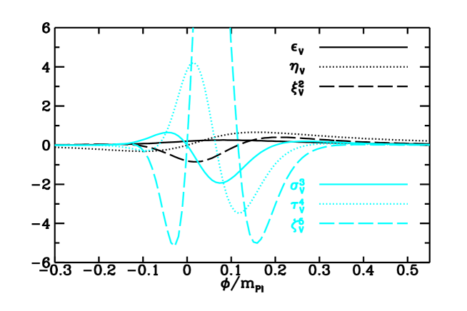
Figure 2: The first six slow-roll parameters.

Given the approximation of linear perturbation theory, the perturbation spectrum can be computed exactly taking the inflationary dynamics into account by using the mode equation formalism of Mukhanov [11]. Numerical solution of this equation was described by Grivell and Liddle [12] and Wang et al. [8]. The scalar and tensor perturbations generated by this potential are shown in Fig. 3. We also show the result of the best available semi-analytic technique as described above, which uses numerical solution of the background field equations as input to the Stewart–Lyth formula and which gives an error of more than ten percent at some $k$. We see that the matter power spectrum is very far from the scale-invariant form, featuring a sharp downturn and then bending back up again. In fact, this deviation from scale-invariance is already too large to be permitted by observational data; for example, in a COBE-normalized CDM-like cosmology the perturbations at $8h^{-1}$ Mpc are only $\sigma_{8}\simeq 0.3$. It still serves as a useful example however.

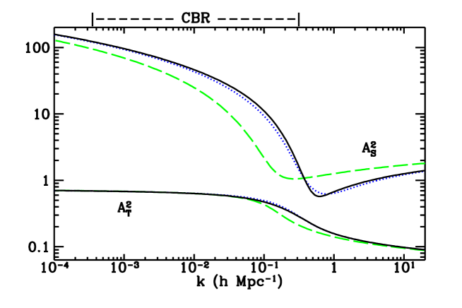
Figure 3: The perturbation spectra obtained by mode equation integration (solid curves) compared to the semi-analytic results (dotted curves) and the lowest-order analytic results (dashed curves). Since the amplitude of the power spectra are proportional to the unknown parameter $\Lambda$ in the potential, $A_{S}^{2}$ and $A_{T}^{2}$ may be adjusted up and down by a common factor. Since inflation is terminated by hand, the spectra can also be shifted left or right. Shown in the figure are the spectra analyzed in subsection 5.1. The spectra analyzed in subsection 5.2 are shifted to the left by a factor of 30 so that the dip in $A_{S}^{2}$ is near $k=0.02h$ Mpc^-1.

Any set of observations will be able to probe only a range of scales, and we shall use the capabilities of the Planck satellite as a benchmark. Planck can probe the microwave anisotropy multipoles from the quadrupole $\ell=2$ up to around $\ell=2000$. The corresponding $k$ range sampled is from $k=a_{0}H_{0}$ to $k=1000\,a_{0}H_{0}$. Using $a_{0}H_{0}=h/3000\,{\rm Mpc}^{-1}$, the range of $k$ probed by Planck is shown in Fig. 3. We see that in fact Planck would be able to see more or less to the bottom of the dip, but not the subsequent rise. So the part of the spectrum to be probed does not contain any very strong features. Fig. 4 shows the predicted $C_{\ell}$ curves, both exact and approximate, calculated using a modified version of the cmbfast code [13]. The slight differences from the equivalent figure in Ref. [8] are presumably from slightly different choices of parameters such as the baryon density. The basic slow-roll method does extremely poorly.

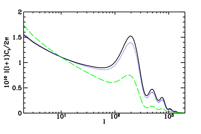
Figure 4: Predicted microwave anisotropies from the power spectra computed under different assumptions summarized in Table 1: from top to bottom they are numerical, semi-analytic, and lowest-order analytic, corresponding to the scalar and tensor spectra shown in Fig. 3.

To illustrate how to recognize when reconstruction is impossible, we shall later consider the case where the scales left the horizon a little further down the scalar field potential, corresponding to shifting the spectrum leftwards by a factor of 30 and bringing the main feature of the spectrum into the observable range.

4 The Reconstruction Procedure

In this section we review the general reconstruction procedure, and extend results for high derivatives of $V$ to higher-order in slow-roll than previously given. Perturbative reconstruction requires that one fits an expansion, usually a Taylor series of the form

$$\ln A_{S}^{2}(k) = \ln A_{S}^{2}(k_{*})+(n_{*}-1)\ln\frac{k}{k_{*}}+\frac{1}{2}\,\left.\frac{dn}{d\ln k}\right|_{*}\ln^{2}\!\frac{k}{k_{*}}$$ (4.1)

$$+\frac{1}{6}\left.\frac{d^{2}n}{d(\ln k)^{2}}\right|_{*}\ln^{3}\!\frac{k}{k_{*}}+\frac{1}{24}\left.\frac{d^{3}n}{d(\ln k)^{3}}\right|_{*}\ln^{4}\!\frac{k}{k_{*}}+\cdots\,,$$

to the observed spectrum in order to extract the coefficients, where stars indicate the value at $k_{*}$. The scale $k_{*}$ is most wisely chosen to be at the (logarithmic) center of the data, so we take $k_{*}=0.01\,h$ Mpc^-1.

How far the series should be taken is governed by how many of the coefficients can be obtained with error bars inconsistent with zero. Planck can in principle measure the $C_{\ell}$ at the percent level of much of its range, though degeneracies with other parameters will weaken the determination of the spectrum somewhat. This sets a ballpark figure for how far the series should go, and for almost all known inflation models only the amplitude and spectral index are required.

In general one should similarly fit the tensor amplitude. The relative amplitude of tensors and scalars is important for reconstruction. If more information about the tensors can be determined than just the amplitude, then the extra information is degenerate with information in the scalars and the consistency relations can be tested, though it seems extremely unlikely that observations will permit this [2, 14, 15].

From these, we reconstruct the potential, using the equations set down in Ref. [2] plus similar equations for $V^{\prime\prime\prime}$ and $V^{\prime\prime\prime\prime}$. This requires the exact relation connecting changes in $\phi$ with changes in $k$ [2],

$$\frac{d\phi}{d\ln k}=\frac{m_{{\rm Pl}}^{2}}{4\pi}\frac{H^{\prime}}{H}\frac{1}{\epsilon-1}\simeq\sqrt{\frac{R_{*}}{4\pi}}\,(1+R_{*})\,,$$ (4.2)

The reconstruction equations, using the notation $n_{*}^{(i)}$ to indicate $\left.d^{i}n/d\ln k^{i}\right|_{*}$ and $R_{*}=A_{T}^{2}(k_{*})/A_{S}^{2}(k_{*})$, are

$$m_{{\rm Pl}}^{-4}\,V(\phi_{*}) \simeq \frac{75}{32}A_{S}^{2}(k_{*})R_{*}\left\{1+\left[0.21R_{*}\right]\,\right\}$$

$$m_{{\rm Pl}}^{-3}\,V^{\prime}(\phi_{*}) \simeq -\frac{75\sqrt{\pi}}{8}A_{S}^{2}(k_{*})R_{*}^{3/2}\left\{1-\left[0.85R_{*}-0.53(1-n_{*})\right]\,\right\}$$

$$m_{{\rm Pl}}^{-2}\,V^{\prime\prime}(\phi_{*}) \simeq \frac{25\pi}{4}A_{S}^{2}(k_{*})R_{*}\left\{9R_{*}-1.5(1-n_{*})\phantom{n_{*}^{(1)}}\right.$$

$$\left.-\left[24.3R_{*}^{2}+0.25(1-n_{*})^{2}-14.8R_{*}(1-n_{*})-1.6\,n_{*}^{(1)}\right]\,\right\}$$

$$m_{{\rm Pl}}^{-1}\,V^{\prime\prime\prime}(\phi_{*}) \simeq -\frac{75\pi^{3/2}}{4}A_{S}^{2}(k_{*})R_{*}^{1/2}\left\{24R_{*}^{2}-8R_{*}(1-n_{*})-n_{*}^{(1)}\right.$$

$$+\left[91R_{*}^{2}(1-n_{*})-9.2R_{*}(1-n_{*})^{2}-128R_{*}^{3}\right.$$

$$\left.\left.+12.3R_{*}\,n_{*}^{(1)}+0.03(1-n_{*})\,n_{*}^{(1)}-1.1n_{*}^{(2)}\right]\,\right\}$$

$$V^{\prime\prime\prime\prime}(\phi_{*}) \simeq 75\pi^{2}A_{S}^{2}(k_{*})\left\{60R_{*}^{3}-30R_{*}^{2}(1-n_{*})-4.5R_{*}\,n_{*}^{(1)}\right.$$ (4.3)

$$+2R_{*}(1-n_{*})^{2}-0.25(1-n_{*})\,n_{*}^{(1)}+\ 0.5\,n_{*}^{(2)}$$

$$+\left[-524R_{*}^{4}+446R_{*}^{3}(1-n_{*})+0.55\,n_{*}^{(3)}\right.$$

$$+0.02(n_{*}^{(1)})^{2}-83.8R_{*}^{2}(1-n_{*})^{2}+65.7R_{*}^{2}\,n_{*}^{(1)}$$

$$+1.6R_{*}(1-n_{*})^{3}-6.8R_{*}\,n_{*}^{(2)}-0.5(1-n_{*})\,n_{*}^{(2)}$$

$$\left.\left.+0.1(1-n_{*})^{2}\,n_{*}^{(1)}-11.1R_{*}(1-n_{*})n_{*}^{(1)}\phantom{R_{*}^{2}}\right]\right\}$$

We can assign a bookkeeping parameter to keep track of the order of the terms appearing in Eq. (4). $R_{*}$ and $1-n_{*}$ is of order 1, and $n_{*}^{(j)}$ is of order $j+1$. One can see that Eq. (4) is arranged so that the higher-order corrections appear in square brackets. Since the fit we use for the scalar power spectrum only goes up to $n_{*}^{(2)}$, we have no information about $n_{*}^{(3)}$, hence for consistency we only use the lowest-order expression for $V^{\prime\prime\prime\prime}$.

$R_{*}$, $n_{*}$, $n_{*}^{(1)}$, $\ldots$ are to be determined from observations. Fortunately, parameter estimation from the microwave background has been explored in some detail [14, 15]. We shall use error estimates for Planck assuming polarized detectors are available, following the analysis of Zaldarriaga et al. [15]. Most analyses have assumed that $R_{*}$ and $n_{*}$ are the only parameters needed to describe the spectra. In a related publication [16], we have generalized their treatment to allow the power spectrum to deviate from scale-invariance. Including extra parameters leads to a deterioration in the determination of all the parameters, as it introduces extra parameter degeneracies. Fortunately, for most parameters the uncertainty is not much increased by including the first few derivatives of $n$ [16], but we have found that the parameter $n$ itself has a greatly increased error bar. If a power-law is assumed it can be determined to around $\Delta n\simeq 0.004$ [15, 16], but including scale dependence increases this error bar by a factor of ten or more. Notice that unless one assumes a perfect power-law behaviour, this increase in uncertainty is applicable even if the deviation from power-law behaviour cannot be detected within the uncertainty.

From Ref. [16], an estimate of the relevant uncertainties is

$$\Delta(R_{*})\simeq 0.004\;\; \;\;\Delta n\simeq 0.14$$ ;

$$\Delta(dn/d\ln k)\simeq 0.04\;\; \;\;\Delta[d^{2}n/d(\ln k)^{2}]\simeq 0.005\,.$$ ; (4.4)

Note that $r_{{\rm ts}}$ in Ref. [16] is 14 times $R_{*}$.

5 Two Reconstruction Examples

In this section we consider two reconstruction attempts of regions of the potential in Fig. 1. One is successful and the other unsuccessful. We demonstrate that this is to be expected and is perfectly consistent with the reconstruction procedure we have adopted, indicating that it is virtually impossible to misconstruct the potential.

5.1 Successful reconstruction

In this subsection we reconstruct the potential shown in Fig. 1 that led to the spectra of Fig. 3. We find that the observational errors dominate over the errors introduced by using the slow-roll approximations for the spectra. We do not agree with claims in Ref. [8] that the breakdown of the slow-roll approximation for this potential illustrates that reconstruction is not valid for general potentials. We also find that, as expected, the shape of the potential is better determined than the amplitude.

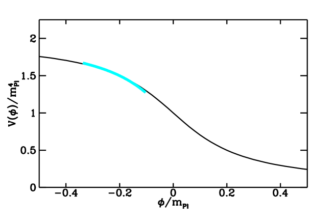
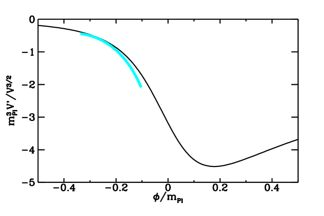
Figure 5: The original potential is compared with the fragment reconstructed from Eq. (4) using the parameter determination in Eq. (5.1). The lower figure is the reconstructed $m_{Pl}^{3}V^{\prime}/V^{3/2}$. The difference between the reconstructed fragments and the true potential is due to the use of the slow-roll expansion in reconstruction.

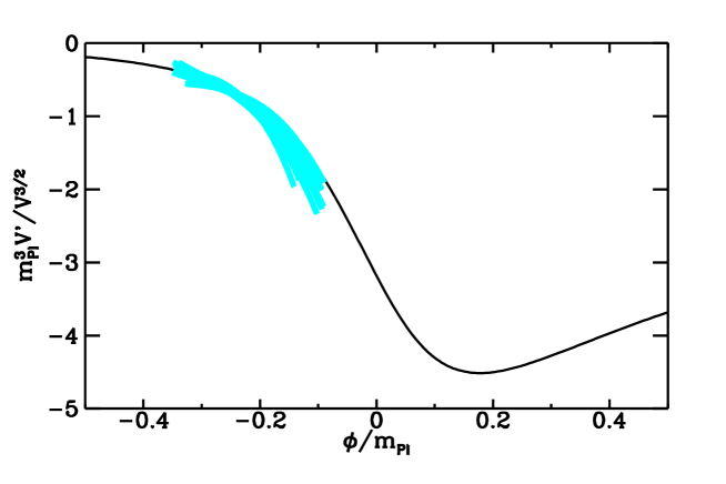
Figure 6: A set of ten reconstructed potential fragments compared with the true potential. The spread in the reconstructed potentials compared to the reconstructed potential in Fig. 5 illustrated our point that the uncertainty in the parameter determination will overwhelm the error introduced by using the slow-roll formalism in reconstruction.

To estimate the errors introduced by the slow-roll formalism, we treat the exact power spectra of Fig. 3 as the ‘observations’, and imagine that we do not know the potential from which they derive. We shall later use estimated uncertainties assuming the spectra are measured via the microwave anisotropies, but for now we shall imagine that the power spectra have been measured exactly in order to assess the errors arising from uncertainties in the theoretical power spectrum determination.

We have fit a Taylor expansion of the above form to the exact spectrum, using $k_{*}$ as above, and found the following results:

$$\ln A_{S}^{2}(k_{*})=3.84\quad;\quad R_{*}=0.014\quad;$$

$$n_{*}=0.579\quad;\quad\left.\frac{dn}{d\ln k}\right|_{*}=-0.134\quad;\quad\left.\frac{d^{2}n}{d(\ln k)^{2}}\right|_{*}=-0.052\ .$$ (5.1)

From the estimated observational uncertainties of Eq. (4), we see that all these coefficients are successfully determined at high significance and a simple “chi–by–eye” demonstrates that the spectrum reconstructed from these data is an adequate fit to the observed spectrum. This stresses the point that the more unusual a potential is, the more information one is likely to be able to extract about it, though the uncertainties on the individual pieces of information may be greater.

We reconstruct the potential in a region about $\phi_{*}=-0.22$ (the reconstruction program does not determine $\phi_{*}$), the width of the region given via Eq. (4.2). The results for the reconstructed potential without observational errors are shown in Fig. 5, where it can immediately be seen that the reconstruction has been very successful in reproducing the main features of the potential while perturbations on interesting scales are being developed.

Thus far we have assumed perfect observations, but of course in practice the measurement of the power spectrum is subject to observational errors. To illustrate visually the effect of the observational errors, we use a Monte Carlo procedure where we draw ‘observed’ parameter values from gaussian distributions about the true value with the appropriate variance. These observed parameters, which include fully the effects of cosmic variance and the modelled instrument noise, are then fed into the reconstruction process. Fig. 6 shows ten such reconstructions about the true value. The uncertainty is indicated by the wide spread in the results. Note the width of the reconstructed region is correlated with the height of the potential; if the observed $R_{*}$ happens by chance to be low the potential is lower and flatter, so the field rolls more slowly as the perturbations are generated.

The uncertainty is dominated by that of $A_{T}^{2}(k_{*})$; although the gravitational waves are detectable in this model, it is only about a three-sigma detection and the error bar is thus large. Since the overall magnitude of the potential is proportional to $A_{T}^{2}$, the visual impression is of a large uncertainty.

Fortunately, information in combinations of the higher derivatives is more accurately determined. Fig. 6 also shows the reconstruction of $V^{\prime}/V^{3/2}$ with observational errors; this combination is chosen as it is independent of the tensors to lowest order. Not only is it reconstructed well at the central point, but both the gradient and curvature are well fit too, confirming useful information has been obtained about not just $V^{\prime\prime}$ but $V^{\prime\prime\prime}$ as well, which is only possible because of the extra information contained in the scale-dependence of the power spectrum. So despite the poor visual impression given by Fig. 6, rather accurate information is being obtained about the potential.

To compare these observational errors with the purely theoretical errors of the slow-roll approximation, one can compare to Fig. 5. From this we conclude that the error introduced by using the bessel function approximation in reconstruction is a small part of the error budget.

5.2 An example where reconstruction is impossible

What we have seen in the example of Subsection 5.1 is that despite slow-roll not working very well, and hence generating significant errors in the normal estimation of the power spectrum, the reconstructed potential still looks very good, especially in the light of expected observational error bars. The main reason for this is that although the spectrum is quite far from scale-invariance, it could still be reasonably fit by just a few terms in the Taylor expansion.

The truly awkward situation would be a spectrum which could not be adequately fit that way, for then perturbative reconstruction would break down. This is no surprise—there is always a limit beyond which a perturbative process cannot be taken. An example, alluded to above, would be if inflation ended just a little later on the potential we have been considering, so that the spectrum is shifted to the left bringing the minimum into the observable range.

We have examined this case and found that indeed the spectrum cannot be fit by a Taylor series to any reasonable order. That reconstruction fails is completely obvious, because we can’t even start. There is no danger of trying to carry out a reconstruction, and obtaining an answer which has no connection to reality. If the observations take this unfortunate turn, then one has a number of options to try. Perhaps single-field inflation is not correct at all, and some other theory such as topological defects or isocurvature fits better. Or perhaps we do believe that a complicated inflaton potential is at work, in which case a non-perturbative technique (e.g. fitting the power in different wavebands) would be more appropriate. Or a multi-field inflation model might be responsible, and one could test them on a model-by-model basis to see if they were compatible with the data.

6 Conclusions

We have found that a complicated potential, such as the example used by Wang et al. [8], would be a boon to reconstruction of the inflaton potential, as it would provide extra information accessible to observations, in the form of scale-dependence of the density perturbations. Such potentials are also more likely to have tensor modes at a detectable level, which is required for a complete reconstruction to be performed.

We have analyzed the impact of observational errors on the reconstruction, and conclude that any theoretical errors from use of the slow-roll equations are likely to be sub-dominant. One might even be able to test this be solving the mode equation for the reconstructed potential, though we have not tried to pursue that route here.

Finally, it has always been clear that there must be some limits to the applicability of perturbative reconstruction, although it does a good job even for the Wang et al. potential. However, such a failure should be immediately evident from the data, as one would not be able to successfully match observations with a truncated Taylor series expansion of the power spectra. It would appear, therefore, that there is no danger that perturbative reconstruction might appear to be working, but in fact be producing an irrelevant potential.

References

- [1] E. J. Copeland, E. W. Kolb, A. R. Liddle and J. E. Lidsey, Phys. Rev. Lett. 71, 219 (1993), Phys. Rev. D 48, 2529 (1993), 49, 1840 (1994); M. S. Turner, Phys. Rev. D 48, 5539 (1993).
- [2] J. E. Lidsey, A. R. Liddle, E. W. Kolb, E. J. Copeland, T. Barreiro and M. Abney, Rev. Mod. Phys. 69, 373 (1997).
- [3] A. R. Liddle and D. H. Lyth, Phys. Rep. 231, 1 (1993).
- [4] D. S. Salopek and J. R. Bond, Phys. Rev. D 42, 3936 (1990).
- [5] A. R. Liddle and D. H. Lyth, Phys. Lett. B 291, 391 (1992).
- [6] A. R. Liddle, P. Parsons and J. D. Barrow, Phys. Rev. D 50, 7222 (1994).
- [7] E. D. Stewart and D. H. Lyth, Phys. Lett. B 302, 171 (1993).
- [8] L. Wang, V. F. Mukhanov and P. J. Steinhardt, Phys. Lett. B 414, 18 (1997).
- [9] E. W. Kolb and S. Vadas, Phys. Rev. D 50, 2479 (1994).
- [10] A. D. Linde, Phys. Lett. B 259, 38 (1991), Phys. Rev D 49, 748 (1994); E. J. Copeland, A. R. Liddle, D. H. Lyth, E. D. Stewart and D. Wands, Phys. Rev D 49, 6410 (1994).
- [11] V. F. Mukhanov, Pis’ma Zh. Eksp. Teor. Fiz. 41, 402 (1985) [Sov. Phys. JETP Lett. 41, 493 (1985)], Zh. Eksp. Teor. Fiz. 94, 1 (1988) [Sov. Phys. JETP 67, 1297 (1988)].
- [12] I. J. Grivell and A. R. Liddle, Phys. Rev. D 54, 7191 (1996).
- [13] U. Seljak and M. Zaldarriaga, Astrophys. J. 469, 437 (1996).
- [14] G. Jungman, M. Kamionkowski, A. Kosowsky and D. N. Spergel, Phys. Rev. D 54, 1332 (1996); J. R. Bond, G. Efstathiou and M. Tegmark, Mon. Not. R. Astron. Soc. 291, L33 (1997).
- [15] M. Zaldarriaga, D. Spergel and U. Seljak, Astrophys. J. 488, 1 (1997).
- [16] E. J. Copeland, I. J. Grivell and A. R. Liddle, Sussex preprint astro-ph/9712028 (1997).