Cherenkov-drift emission mechanism

Abstract

Emission of a charged particle propagating in a medium with a curved magnetic field is reconsidered stressing the analogy between this emission mechanism and collective Cherenkov-type plasma emission. It is explained how this mechanism differs from conventional Cherenkov, cyclotron or curvature emission and how it includes, to some extent, the features of each of these mechanisms. Presence of a medium supporting subluminous waves is essential for the possibility of wave amplification by particles streaming along the curved magnetic field with a finite curvature drift. We suggest an analogy between the curvature drift emission and the anomalous cyclotron-Cherenkov emission. Treating the emission in cylindrical coordinates in the plane-wave-like approximation allows one to compute the single particle emissivity and growth rate of the Cherenkov-drift instability. We compare the growth rates calculated using the single particle emissivity and using the dielectric tensor of one dimensional plasma streaming along the curved field. In calculating the single particle emissivity it is essential to know the normal modes of the medium and their polarization which can be found from the dielectric tensor of the medium. This emission mechanism may be important for the problem of pulsar radio emission generation.

1 April 1997

I Introduction

Studies of relativistic strongly magnetized plasma in astrophysical setting (like pulsar magnetosphere) have shown the possibility of a new mechanism of electromagnetic wave generation. This new mechanism, which combines features of conventional Cherenkov, cyclotron and curvature radiation, deserves more detailed consideration from the fundamental physics point of view. Besides investigating the physical nature of this process, we also reconcile different available approaches to this problem.

In this work we discuss this novel emission mechanism of a charged particle streaming with relativistic velocity along curved magnetic field line in a medium. A weak inhomogeneity of the magnetic field results in a curvature drift motion of the particle perpendicular to the local plane of the magnetic field line. A gradient drift (proportional to ${\bf\nabla\cdot B}$) is much smaller than the curvature drift and will be neglected. When the motion of the particle parallel to the magnetic field is ultrarelativistic the drift motion even in the weakly inhomogeneous field can become weakly relativistic resulting in a new type of generation of electromagnetic, vacuumlike waves. Presence of three ingredients ( strong but finite magnetic field, inhomogeneity of the field and a medium with the index of refraction larger than unity) is essential for the emission. We will call this mechanism Cherenkov-drift emission stressing the fact that microphysically it is virtually Cherenkov-type emission process.

Conventional consideration of the curvature emission ([1], [2], [3], [4]) emphasize the analogy between curvature emission and conventional cyclotron emission. To our opinion this approach, though formally correct, has limited applicability and misses some important physical properties of the emission mechanism. In a separate approach Kazbegi et al. [5] considered this process calculating a dielectric tensor of the inhomogeneous magnetized medium, thus treating the emission process as a collective effect. They showed that maser action is possible only if a medium supports subluminous waves. In this work we show how these two approaches can be reconciled and argue that the dielectric tensor approach, which treats the Cherenkov-drift emission as a collective process, has a wider applicability.

The interplay between cyclotron (or synchrotron) and Cherenkov radiation has been a long-standing matter of interest. Schwinger et al. [6] discussed the relation between these two seemingly different emission mechanisms. They showed that conventional synchrotron emission and Cherenkov radiation may be regarded as respectively limiting cases of $|n-1|\,\ll\,1$ and $B=\,0$ of a synergetic (using the terminology of Schwinger et al. [6]) cyclotron-Cherenkov radiation. In another work [7] this analogy has been discussed to include cyclotron-Cherenkov emission at the anomalous Doppler resonance. An important new aspect of our work (as compared with [6] and [7] ) is that we take into account inhomogeneity of the medium.

Physical origin of the emission in the case of Cherenkov-type and synchrotron-type processes is quite different. In the case of Cherenkov-type process the emission may be attributed to the electromagnetic polarization shock front that develops in a dielectric medium due to the passage of a charged particle with speed larger than phase speed of waves in a medium. It is virtually a collective emission process. In the case of synchrotron-type process, the emission may be attributed to the Lorentz force acting on a particle in a magnetic field. Cherenkov-type emission is impossible in vacuum and in a medium with the refractive index smaller than unity.

Cyclotron emission at the anomalous Doppler effect (cyclotron-Cherenkov emission) is an interesting example of Cherenkov-type emission process of a particle in a magnetic field. It is impossible in vacuum and requires a superluminous motion of a particle along the magnetic field. Thus, the emission at the anomalous Doppler effect is attributed to the polarization shock front that a spiraling particle induces in a medium. In our opinion, the Curvature-drift emission may be viewed as a Cherenkov-type emission that bears the same relation to the conventional curvature emission as the cyclotron emission at the anomalous Doppler effect bear to the conventional cyclotron emission.

In this work we consider a Curvature-drift emission of the particles in the ground gyrational state. It is possible to obtain the emissivity for particles in excited gyrational state by the method of dielectric tensor [8]. Then, conventional cyclotron (cyclotron-Cherenkov), Cherenkov and curvature emission mechanisms may be viewed as corresponding limits of the Cherenkov-drift mechanism in the cases of homogeneous magnetic field (in a medium), medium without magnetic field, and inhomogeneous magnetic field without a medium.

In Section II we discuss our set up of the problem and how it differs from the previous consideration. In Section III we calculate a single particle emissivity of the Cherenkov-drift mechanism and find the growth for kinetic beam instability toward excitation of electromagnetic waves at the Cherenkov-drift resonance. Then the results are compared with those obtained by the dielectric tensor method.

II Description of a model

Let us consider concentric coplanar circular magnetic field lines populated with charged particles streaming relativistically along the curved magnetic field (Fig. 1).

FIG. 1.: Geometry of the considered problem. The magnetic field lines are concentric coplanar circular arcs with the radius of curvature much larger than the size of the region.

The magnetic field is assumed to be very strong, so that the particles are in their ground gyrational state (zeroth Landau level). Next we introduce a cylindrical system coordinates $r,\phi,x$ with the unit vector ${\bf e}_{\phi}$ along the local magnetic field, ${\bf e}_{x}$ perpendicular to the osculating plane of the magnetic field and ${\bf e_{r}}={\bf e}_{\phi}\times{\bf e}_{x}$. We will limit the region under consideration to have the size along the $r$ axis $\delta r$ much smaller than the typical radius of curvature of the field lines in the region ($\delta r\ll R_{B}$) and much larger than the typical wave length of the considered waves ($\delta r\gg\lambda$). This physical picture may be considered as an approximation to the region of the open field lines of the pulsar magnetosphere. The curved dipole field can be locally approximated by the circular field with the radius of curvature $R_{B}$. The typical radius of curvature $R_{B}\approx 10^{9}$ cm and the wave length of the emitted radiation is of the order of meters $\lambda\approx 10^{2}$ cm. Then for the size of the region satisfying the condition $10^{2}{\rm cm}\ll\delta r\ll 10^{9}$ cm, it can be considered as homogeneous.

Next, we assume, that the collective interactions of the particles with waves propagating in the system may be described using a dielectric tensor. Then, for a given wave mode, all the particles may be separated in the plasma particles, i.e. those particles that interact with the wave nonresonantly, and resonant particles. We expect that outgoing electromagnetic modes generated by some fluctuating currents at smaller radii will interact with resonant particle and will be amplified as they propagate through the interaction region (see Fig. 1).

We wish to find the specific intensities for emission of electromagnetic waves by the resonant particles in such a system. This may be done by calculating the work done by the extraneous current associated with the resonant particle moving along a given trajectory ([4]) or by calculating the dielectric tensor of the medium. Below we discuss in details the calculations using the former method and compare it with the results obtained using the dielectric tensor.

In a curved magnetic field a particle with relativistic Lorentz factor $\gamma$ streaming along the field line experiences a drift in the $x$ direction with velocity

$$u_{d}={\gamma_{\phi}v_{\phi}^{2}\over\omega_{B}R_{B}},$$ (1)

where $\omega_{B}=\,q\,B/(m\,c)$ is the nonrelativistic gyrofrequency, $q$ is charge of the particle, $m$ is its mass and $c$ is the speed of light.

With the instantaneous 3-velocity ${\bf v}=\{0,v_{\phi},u_{d}\}$ the radius vector of the particle is

$${\bf r}(t)=\{R_{B},v_{\phi}t,u_{d}t\}.$$ (2)

The current density associated with the charge is

$${\bf j}({\bf r},t)=q{\bf v}\delta({\bf r}-{\bf r}(t)).$$ (3)

We next find the Fourier transform of the current (3) in cylindrical system of coordinates by expanding the current density in real space (3) in terms of cylindrical waves $\exp\left(-i(k_{r}r+k_{x}x+m\phi)\right)$ (m - integer) :

$${\bf j}(\omega,{\bf k})=\int_{-\infty}^{\infty}dt\int d{\bf r}\,{\bf j}({\bf r},t)\exp\left(i(\omega t-k_{r}r-k_{x}x-m\phi)\right).$$ (4)

Using the relation

$$\int_{-\infty}^{\infty}dt\exp\left(i\alpha t\right)=2\pi\delta(\alpha)$$ (5)

and the radius vector (2) we find the Fourier image of the current:

$${\bf j}(\omega,{\bf k})=2\pi q{\bf v}\exp\{-ik_{r}R_{B}\}\delta(\omega-k_{\phi}v_{\phi}-k_{x}u_{d}),$$ (6)

where we introduced $k_{\phi}=m/R_{B}$. For $m\gg 1$ we can assume that $k_{\phi}$ is continuous.

The condition, that the size of the region considered is much larger than the wave length places a lower limit on the wave frequency in (6):

$$\omega\gg\Omega,$$ (7)

where $\Omega=v_{\phi}/R_{B}$ is the angular frequency of the particle’s rotation along the circular magnetic field. The condition (7) also vindicates the assumption $m\gg 1$.

The expansion (4) in cylindrical coordinates has a limited applicability [9]. Generally, in cylindrical coordinates the normal modes will be expressed in terms of Bessel-type functions. For the nonresonant modes we can use WKB approximation to the radial dependence of normal modes (this is equivalent to the tangent expansion of Bessel functions when argument is larger and not close to the order). On the other hand, for the resonant modes the argument of Bessel functions is close to the order, so that the WKB approximation (or expansion in tangents) is not applicable. In this case we can use Airy function approximation to Bessel function, which, in turn, has a wave-like approximation for the interaction of subluminous waves with the particles moving with the speed larger than the speed of light in a medium (this corresponds to the Airy function expansion argument is larger than the order). It is shown in [9] that for the large argument expansionof Airy function to apply it is required that (i) $n-1\gg 1/\gamma^{2}$ and (ii) $(n-1)m^{2/3}\geq 1$ (here $n$ is the refractive index, $\gamma$ is the Lorentz factor of the resonant particle. Summarizing the above: expansion (4) is valid in the two different regimes: (i) for the nonresonant modes, (ii) for the resonant modes when $n-1\gg 1/\gamma^{2}$ and $(n-1)m^{2/3}\geq 1$. In what follows we assume that the conditions for the expansion (4) are satisfied.

An important difference of this approach from the one used in [1] and [3] is that we calculate the transition current in cylindrical coordinates, while in [1], and [3] the transition current was calculated in Cartesian coordinates. In adopting Cartesian coordinates with planar normal modes the interaction length for an individual electron, $\approx R_{B}/\gamma_{b}$, was essentially coextensive with region over which the waves could possibly interact with any electron. This introduces a strict constraint on the particle-wave interaction and precluded a strong amplification under all circumstances because the wave would have to grow substantially during a very short interaction in a manner that could not be easily quantified. The second major difference from [1] and [3] is that we consistently take dispersion into account.

The major advantage of cylindrical system of coordinates is that the only inhomogeneity present in the problem, the weak inhomogeneity of the direction of magnetic field, can be effectively eliminated by transforming to the cylindrical system of coordinates. It is the choice of cylindrical coordinates that allows one to describe the weakly inhomogeneous system by the homogeneous (independent of r ) set of equation, but in the curved coordinates. The use of cylindrical waves with the phase dependence of the form $\exp\left(i(\omega t-k_{r}r-k_{x}x-m\phi)\right)$. has a limited applicability, but allows for simple estimate of the Cherenkov-drift emissivity and growth rate.

III Cherenkov-drift emissivity and amplification

In this section we calculate the growth rate of the Cherenkov-drift instability by finding the Cherenkov-drift emissivity for the single particles on the zeroth Landau level streaming along the curved magnetic field. We then compare it with the calculations done using the dielectric tensor of a plasma in a curved magnetic field. The results of both calculations, obviously, coincide.

With the known current density, the energy radiated by the particle into a given wave mode $\alpha$ is given by ([4], Eq. (3.18))

$$U^{\alpha}=4\pi R_{E}^{\alpha}({\bf k})\left|{\bf e}^{\ast\alpha}\cdot{\bf j}(\omega^{\alpha},{\bf k})\right|^{2},$$ (8)

where ${\bf e}^{\alpha}$ is the polarization vector of the emitted mode and $R_{E}^{\alpha}$ is the ratio of electric to total energy in the wave, as defined by [4].

To find the energy radiated one has first to determine the normal modes of the medium and find their polarization. In contract to the vacuum case, where one is free to chose arbitrary combination of plane transverse electromagnetic waves as normal modes, in a medium the normal modes must be the eigenvectors of the corresponding dispersion equation.

To determine the the normal modes and their polarization we must solve the dispersion equation

$$Det\left|\Lambda_{lm}\right|=0,\hskip 14.45377pt\Lambda_{lm}=(k^{2}\delta_{lm}-k_{l}k_{m}){c^{2}\over\omega^{2}}-\epsilon_{lm},$$ (9)

where $\epsilon_{lm}$ is the dielectric tensor of the medium. Dielectric tensor for a one dimensional plasma streaming along the strong magnetic field has been calculated in [5], [9].

Dispersion equation (9) is very complicated - all the nine components of the matrix $\Lambda_{lm}$ are nonzero. This is different from the case of a plasma in a homogeneous magnetic field, where, due to the cylindrical symmetry around magnetic field, some components of $\Lambda_{lm}$ could be set to zero without a loss of generality.

A Polarization of Waves in Anisatropic Dielectric

Below we will restrict our consideration to the case of electron-positron plasma with the same distribution functions streaming along a superstrong magnetic field.

1 Infinitely Strong Magnetic Field

In the infinitely strong magnetic field the dielectric tensor is

$$\epsilon_{ij}=\left(\begin{array}[]{ccc}1&0&0\\ 0&1-K&0\\ 0&0&1\end{array}\right)$$ (10)

where

$$K={4\pi q^{2}\over m_{e}}\int{dp_{\phi}\over\gamma^{3}}{f(p_{\phi})\over(\omega-\Omega m)^{2}}={4\pi q^{2}\over\omega}\int dp_{\phi}{v_{\phi}\over\omega-\Omega m}{\partial f^{(0)}\over\partial p_{\phi}}$$ (11)

$f(p_{\phi})$ is a one dimensional distribution function.

The dispersion equation (11) may be factored for the dispersion relations of the t-mode, with the electric field perpendicular to the k - B plane, and lt-mode, with the electric field in the k - B plane (Fig. 2):

$$n^{2}=1,\hskip 72.26999pt{\bf e}^{(t)}={1\over n_{\perp}}\{-n_{x},0,n_{r}\}\mbox{}$$ (12)

$$n_{\phi}^{2}=1-{n_{\perp}^{2}\over 1-K},\mbox{}$$ (13)

$${\bf e}^{(lt)}={1\over\sqrt{(1-K)^{2}+Kn_{\perp}^{2}}}\{\sqrt{(1-K)(1-K-n_{\perp}^{2})}{n_{r}\over n_{\perp}},-n_{\perp},\sqrt{(1-K)(1-K-n_{\perp}^{2})}{n_{x}\over n_{\perp}}\}$$ (14)

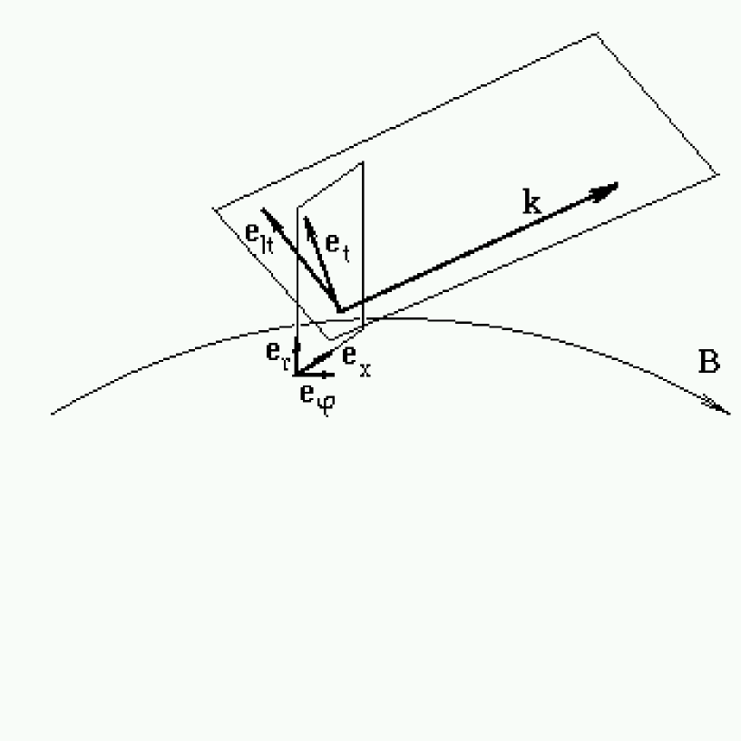
FIG. 2.: Normal modes in the considered medium in the limit of very strong magnetic field. The electric field vector of the $t$-mode is in the plane ${\bf e_{r}}-{\bf e_{x}}$ and the electric vector of the $lt$-mode is orthogonal to ${\bf e}_{t}-{\bf k}$ plane.

These waves are natural analogs of the t- and lt-modes in the case of straight magnetic field lines. The t-mode is purely transverse and the lt-mode is a mixed transverse-longitudinal wave. Generally, in the lt-mode the electric field is not perpendicular to the wave vector, but for teneous plasma in the high frequency limit $K\approx 0$, so that the lt-wave is approximately transverse:

$${\bf e}^{(lt)}={1\over n_{\perp}}\{-n_{r}n_{\phi},n_{\perp},-n_{x}-n_{\phi}\}$$ (15)

2 Finite Magnetic Field

In the finite magnetic field the dielectric tensor is

$$\epsilon_{ij}=\left(\begin{array}[]{ccc}1+2d&0&0\\ 0&1-K&0\\ 0&0&1+2d\end{array}\right)$$ (16)

where for cold plasma $d=\omega_{p}^{2}/\omega_{B}^{2}$. Eq. (17). Dispersion relation is then

$$\left(-(1-K)n_{\phi}^{2}+(1+2d)(1-K-n_{r}^{2}-n_{x}^{2})\right)(1+2d-n_{\phi}^{2}-n_{r}^{2}-n_{x}^{2})=0$$ (17)

which has solutions

$$n^{2}=(1+2d),\hskip 72.26999pt{\bf e}^{(t)}={1\over n_{\perp}}\{-n_{x},0,n_{r}\}\mbox{}$$ (18)

$$n_{\phi}^{2}=(1+2d)\left(1-{n_{\perp}^{2}\over 1-K}\right),\mbox{}$$ (19)

$${\bf e}^{(lt)}\approx{1\over\sqrt{(1-K)^{2}+Kn_{\perp}^{2}}}\{\sqrt{(1-K)(1-K-n_{\perp}^{2})}{n_{x}\over n_{\perp}},-n_{\perp},{n_{r}\over n_{\perp}}\}+O(d)$$ (20)

So that the polarization vectors are the same as in the case of infinitely strong magnetic field within factors $\omega_{p}^{2}/\omega_{B}^{2}$.

B Cherenkov-drift emissivity

With the ${\bf k}$ vector of the emitted transverse waves given by

$${\bf k}=\left\{k_{r},k_{\phi},k_{x}\right\},$$ (21)

we choose the following polarization vectors

$${\bf e^{lt}}={1\over kk_{\perp}}\left\{k_{\phi}k_{r},-k_{\perp}^{2},k_{x}k_{\phi}\right\},\mbox{}$$ (22)

$${\bf e^{t}}={1\over k_{\perp}}\left\{-k_{x},0,k_{r},\right\},$$ (23)

where $k_{\perp}=\sqrt{k_{r}^{2}+k_{x}^{2}}$. This choice of polarization vectors is a limiting case of very strong magnetic field and tenous plasma.

We note, that the separation of the normal modes done in [1], [3], [4] is related not to plane of the real magnetic field, directed along $\phi$, and of the vector ${\bf k}$, but to the plane ${\bf k}-{\bf e_{x}}$. This is justified only in vacuum or in the homogeneous medium where there a freedom in the choice of polarization vectors of the normal modes. In an anizatropic medium the normal modes and their polarizations have to be determined from the dispersion equation.

The eigenvectors (23) are different from those chosen by [3], [4]. The modes chosen in those works follow the analogy between the curvature and synchrotron emission. They are not the normal modes of the medium. The approach of [3], [4], involving vacuum wave polarization and refractive index close but not equal to unity, may be considered as correction to the vacuum curvature emissivity due to presence of a medium when effects of the medium on wave propagation are small. When effects of the medium on wave propagation cannot be considered as small perturbations one has to solve the dispersion relation to find the normal modes and their polarization. This stresses once again the importance of a medium in what we call the Cherenkov-drift emission. Presence of a medium changes the nature of the emitted modes and changes the corresponding emissivities.

With the polarization vectors (23), the single particle probability of emission (per unit volume $d{\bf k}/(2\pi)^{3}$ may be written as a polarization tensor

$$w^{\alpha\beta}({\bf k},{\bf p})={4\pi^{2}q^{2}\over\hbar\omega({\bf k})}F^{\alpha\beta}({\bf k},{\bf p})\delta(\omega-k_{\phi}v_{\phi}-k_{x}u_{d}),\mbox{}$$ (24)

$$F^{\alpha\beta}({\bf k},{\bf p})=\left(\begin{array}[]{cc}A^{2}&iCA\\ -iCA&C^{2}\end{array}\right),\mbox{}$$ (27)

$$A={1\over kk_{\perp}}\left(u_{d}k_{\phi}k_{x}v_{\phi}-k_{\perp}^{2}v_{\phi}\right),\mbox{}$$ (28)

$$C={u_{d}k_{r}\over k_{\perp}},$$ (29)

with $\alpha,\,\beta=t$, $lt$. This form of the emissivity may be compared with [4], Eq. (13.62-13.65), and [3]. There are two main differences: (i) the approximate expressions in [4] and [3] for the single particle emissivity per unit frequency, involving Airy functions, are obtained if the transition current is calculated in Cartesian coordinates, while relations (29) are exact, (ii) the polarization of the normal modes chosen in [4] and [3] are different from ours.

The total emissivity, summed over polarizations, follows from (29):

$$w({\bf k},{\bf p})={4\pi^{2}q^{2}\over\hbar\omega({\bf k})}\left[\left({k_{\phi}k_{x}u_{d}\over kk_{\perp}}-{k_{\perp}v_{\phi}\over k}\right)^{2}+{k_{r}^{2}u_{d}^{2}\over k_{\perp}^{2}}\right]\delta(\omega-k_{\phi}v_{\phi}-k_{x}u_{d}).$$ (30)

The first term in square brackets corresponds to the emission of the lt-mode, second - to the emission of the t-mode.

Next we calculate the growth rate of the Cherenkov drift instability ([4]):

$$\Gamma=\int d{\bf p}w({\bf k},{\bf p})\,\hbar{\bf k}\cdot{\partial f({\bf p})\over\partial{\bf p}}.$$ (31)

Growth rate for the lt-mode is

$$\Gamma^{lt}={4\pi^{2}q^{2}\over m}\int dp_{\phi}\left({k_{\phi}k_{x}u_{d}\over ckk_{\perp}}-{v_{\phi}\over c}{k_{\perp}\over k}\right)^{2}{\partial f(p_{\phi})\over\partial p_{\phi}}\delta\left(\omega-k_{\phi}v_{\phi}-k_{x}u_{d}\right),$$ (32)

and growth rate for the t-mode is

$$\Gamma^{t}={4\pi^{2}q^{2}\over m}\int dp_{\phi}\left({k_{r}u_{d}\over k_{\perp}c}\right)^{2}{\partial f(p_{\phi})\over\partial p_{\phi}}\delta\left(\omega-k_{\phi}v_{\phi}-k_{x}u_{d}\right).$$ (33)

Presence of delta function with the Cherenkov-drift resonance condition without the gyromagnetic term indicates that this is a Cherenkov-type emission process which requires that the medium supports subluminous waves. The necessary condition for the instability is also the same as in the conventional Cherenkov instability: the derivative of the distribution function must be positive at the resonant frequency and wave vector. In physical terms this means that the number of particles with the velocity larger than the phase velocity of the waves exceeds the number of particles with the velocity smaller than the phase velocity of the waves. This once again stresses the Cherenkov-type nature of the emission.

It is clear from (32) and (33) that the growth rate of the t-wave is proportional to the drift velocity and becomes zero in the limit of vanishing drift velocity. As for the lt-wave, it can be excited in the limit of vanishing drift by the conventional Cherenkov mechanism which does not rely on the curvature of the magnetic field lines. We recall, that in the limit of a strong magnetic field and oblique propagation lt-wave has two branches: one superluminous and one subluminous ([10], [11]). On the conventional Cherenkov resonance it is possible to excite only subluminous waves. We note that the choice of polarization vectors of [1], [4] and [3] excludes the excitation of the subluminous branch as well (for which electric field is not perpendicular to the k vector) thus prohibiting any maser action without taking into account drift motion.

The growth rates (33) and (32) may be compared with the calculation done using the antihermitian part of the dielectric tensor [5] . In case of kinetic instability the growth rate is given by ([4])

$$\Gamma=\left.-{(e_{\alpha}^{\ast}\epsilon^{\prime\prime}_{\alpha\beta}e_{\beta})\over{1\over\omega^{2}}{\partial\over\partial\omega}\omega^{2}(e_{\alpha}^{\ast}\epsilon^{\prime}_{\alpha\beta}e_{\beta})}\right|_{\omega=\omega({\bf k})},$$ (34)

where $\epsilon^{\prime}_{\alpha\beta}$ and $\epsilon^{\prime\prime}_{\alpha\beta}$ are hermitian and antihermitian parts of the dielectric tensor, $\omega({\bf k})$ is the frequency of the excited normal mode of the medium, and ${\bf e}$ is its polarization vector.

The relevant components of the antihermitian part of the dielectric tensor follow from [5], [11]:

$$\epsilon^{\prime\prime}_{xx} =-i{4\pi^{2}q^{2}\over\omega c}\int{dp_{\phi}}u_{d}^{2}{\partial f(p_{\phi})\over\partial p_{\phi}}\delta\left(\omega-k_{\phi}v_{\phi}-k_{x}u_{d}\right),\mbox{}$$ (35)

$$\mbox{}\epsilon^{\prime\prime}_{x\phi} =-i{4\pi^{2}q^{2}\over\omega c}\int{dp_{\phi}}u_{d}v_{\phi}{\partial f(p_{\phi})\over\partial p_{\phi}}\delta\left(\omega-k_{\phi}v_{\phi}-k_{x}u_{d}\right)=\epsilon^{\prime\prime}_{\phi x},\mbox{}$$ (36)

$$\mbox{}\epsilon^{\prime\prime}_{\phi\phi} =-i{4\pi^{2}q^{2}\over\omega}\int{dp_{\phi}}v_{\phi}{\partial f(p_{\phi})\over\partial p_{\phi}}\delta\left(\omega-k_{\phi}v_{\phi}-k_{x}u_{d}\right).$$ (37)

Using (34) and (37) we confirm the growth rates (33) and (32) for $v_{\phi}\approx c$.

This approach, involving dielectric tensor of the medium may be considered as a more general, than the one using the single particle emissivities. The dielectric tensor approach takes consistently into account both resonant and nonresonant particles. In calculating the single particle emissivities one still has to calculate the dielectric tensor to find the properties of the emitted normal modes of the medium.

Next we estimate the growth rate for the Cherenkov-drift excitation of electromagnetic waves in the strongly magnetized electron-positron plasma. In the plasma frame the dispersion relations for the transverse modes in the limit $\omega-k_{\phi}v_{\phi}\ll\omega_{B}$ for quasi-parallel propagation ($k_{r},\,k_{x}\ll k_{\phi}$) is

$$\omega=kc\,(1-\delta),\hskip 14.45377pt\delta={\omega^{2}T_{p}\over\omega_{B}^{2}}\,\ll 1,$$ (38)

([5]), where $\omega^{2}=4\pi q^{2}n_{p}/m$ is the plasma frequency of electrons or positrons, $n_{p}$ -density of plasma, $T_{P}$ is effective temperature of plasma in units of $mc^{2}$.

The resonance condition, given by the delta function in Eq. (32), then reads

$${1\over 2\,\gamma_{res}^{2}}-\delta+{k_{r}^{2}\over 2k_{\phi}^{2}}+{1\over 2}\left({k_{x}\over k_{\phi}}-{u_{d}\over c}\right)^{2}=\,0,$$ (39)

where we used $v_{res}=c(1-{1\over 2\,\gamma_{res}^{2}}-{u_{d}^{2}\over 2c^{2}})$. The emission geometry at the Cherenkov-drift resonance is shown in Figs. 3 and 4.

FIG. 3.: Cherenkov-drift emission in the case $\delta\ll u_{d}^{2}/c^{2}$. Drift velocity ${\bf u}_{d}$ is perpendicular to the plane of the curved field line $({\bf B}-{\bf R_{c}}$ plane, ${\bf R_{c}}$ is a local radius of curvature). The emitted electromagnetic waves are polarized along ${\bf u}_{d}$. The emission is generated in the cone centered at the angle $\theta^{em}=u_{d}/c$ and with the opening angle $(2\delta)^{1/2}\ll\theta^{em}$.

FIG. 4.: Emission geometry of the Cherenkov-drift resonance

The maximum growth rate for the t-mode is reached when $k_{x}/k_{\phi}=u_{d}/c$ and the maximum growth rate for the lt-mode is reached when $k_{r}=0$. We also note, that in the excitation of both lt- and t-wave it is the $x$ component of the electric field that is growing exponentially.

Estimating (32) and (33) using $\delta$-function ( max [ ${k_{r}\over k_{\perp}}$ ] $\approx c\sqrt{2\delta}/u_{d}$ and max[${k_{\phi}k_{x}u_{d}\over ckk_{\perp}}-{v_{\phi}\over c}{k_{\perp}\over k}$] $\approx\sqrt{2\delta}$), we wind the maximum growth rates of the t- and lt-modes in the limit $\delta\gg 1/\gamma_{res}^{2}$:

$$\Gamma^{t}=\Gamma^{lt}\approx{2\omega_{p,res}^{2}\delta\over\omega}\left({\gamma^{3}\over 1+u_{d}^{2}\,\gamma^{2}/c^{2}}{\partial f(\gamma)\over\partial\gamma}\right)_{res},$$ (40)

where $\omega_{p,res}$ is the plasma density of the resonant particles.

We estimate the growth rates (40) for the distribution function of the resonant particles having a Gaussian form:

$$f(p_{\phi})={1\over\sqrt{2\pi}p_{t}}\exp\left(-{(p_{\phi}-p_{b})^{2}\over 2p_{t}^{2}}\right),$$ (41)

where $p_{b}$ is the momentum of the bulk motion of the beam and $p_{t}$ is the dispersion of the momentum. Assuming in (40) that $u_{d}\gamma_{b}/c\gg 1$ we find the growth rates

$$\Gamma^{t}=\Gamma^{lt}\approx\sqrt{{2\over\pi}}{\omega_{p,res}^{2}\delta\gamma_{b}\over\omega\gamma_{t}^{2}}{c^{2}\over u_{d}^{2}},$$ (42)

where $\gamma_{b}=p_{b}/(mc),\,\gamma_{t}=p_{t}/(mc)$.

Numerical estimates show, that the growth rate (42) may be large enough to account for the high brightness radiation emission generation in pulsars. For the sake of consistency we leave the detail investigation of the possible application of this radio emission mechanism to pulsar physics for a separate paper.

IV Conclusion

In this paper we considered a new Cherenkov-drift emission mechanism that combines features of the conventional cyclotron, Cherenkov and curvature emission. We argued, that from the microphysical point of view this emission mechanism may be regarded as a Cherenkov-type process in inhomogeneous magnetic field. Considering emission process in cylindrical coordinates we have obtained the single particle emissivities. We also pointed out, that in order to obtain correct expressions for the emissivities it is necessary to use the polarization vectors of the normal modes of the medium. Finally, we calculated the growth rates of the Cherenkov-drift instability in a strongly magnetized electron-positron plasma.

REFERENCES

- [1] R.D. Blandford, MNRAS, 170, 551, (1975)
- [2] V.V. Zheleznyakov & V.E. Shaposhnikov, Aust. J. Phys., 32, 49, (1979)
- [3] Q.H. Luo & D.B. Melrose, MNRAS, 258, 616, (1992)
- [4] Melrose D.B., Plasma astrophysics : nonthermal processes in diffuse magnetized plasmas, New York, Gordon and Breach, (1978)
- [5] A.Z. Kazbegi, G.Z. Machabeli, G.I Melikidze, MNRAS, 253, 377 (1991)
- [6] J. Schwinger, W.Y. Tsai and T. Erber, Ann. Phys., 96, 303, (1976).
- [7] M. Lyutikov, Caltech preprint GRP-459
- [8] M. Ahalkatsi & G. Machabeli G., Plasm. Phys. Contr. Fus. (submitted)
- [9] M. Lyutikov, G.Z. Machabeli & R.D. Blandford, in preparation
- [10] J. Arons & J.J. Barnard, ApJ, 302, 120, (1986)
- [11] M. Lyutikov & G.Z. Machabeli, in preparation.