The range of masses and periods explored by radial velocity searches for planetary companions

Abstract

Radial velocity measurements have proven a powerful tool for finding planets in short period orbits around other stars. In this paper we develop an analytical expression relating the sensitivity to a periodic signal to the duration and accuracy of a given set of data. The effects of windowing are explored, and also the sensitivity to periods longer than the total length of observations. We show that current observations are not yet long or accurate enough to make unambiguous detection of planets with the same mass and period as Jupiter. However, if measurements are continued at the current best levels of accuracy (5 m/sec) for a decade, then planets of Jovian mass and brown dwarfs will either be detected or ruled out for orbits with periods less than $\sim$15 years.

As specific examples, we outline the performance of our technique on large amplitude and large eccentricity radial velocity signals recently discussed in the literature and we delineate the region explored by the measurements of 14 single stars made over a twelve year period by Walker et al. (1995). Had any of these stars shown motion like that caused by the exo-planets recently detected, it would have been easily detected. The data set interesting limits on the presence of brown dwarfs at orbital radii of 5–10 AU. The most significant features in the Walker et al. data are apparent long term velocity trends in 36 UMa and $\beta$ Vir, consistent with super planets of mass of 2 $M_{J}$ in a 10 year period, or 20–30 $M_{J}$ in a 50 year period. If the data are free of long term systematic errors, the probability of just one of the 14 stars showing this signal by chance is about 15%.

Finally, we suggest an observing strategy for future large radial velocity surveys which, if implemented, will allow coverage of the largest range of parameter space with the smallest amount of observing time per star. We suggest that about 10-15 measurements be made of each star in the first two years of the survey, then 2–3 measurements per year thereafter, provided no (or slow) variation is observed. More frequent observations would of course be indicated if such variations were present.

1 Introduction

For nearly two decades most high precision radial velocity surveys of nearby stars were focused on detecting radial velocity variations in stars due to companions with mass and period of Jupiter. The signature would consist of changes in the relative stellar radial velocity with a period of a decade and amplitude of a few tens of meters per second or less, depending on orbital inclination with respect to the solar system. The surprising recent result, triggered by the discovery of 51 Peg B by Mayor & Queloz (1995), has been the finding that as many as 5-10% of solar type stars have companions with mass $<10M_{J}$ and with periods less than $\sim$3 years. No sub-stellar companions with periods longer than $\sim$3 years have so far been detected by radial velocity searches.

Are Jupiter mass companions at longer periods rare, or is it simply the case that current observations do not have the length or sensitivity to see them? Is the theoretical prediction by Boss (1995) correct, that Jovian planets should form preferentially at $>$4-5 AU separations from their primary? Our purpose in this paper is to show what we can learn from velocity data of a given duration and accuracy, to help plan continued programs.

The best measurement errors for a series of radial velocity measurements so far published are those of Butler et al. (1996), who observe a magnitude $V=5$ star and quote an accuracy of 3 m/s for measurements taken over one year. Measurements up until this work have been limited to a lower accuracy standard of about 15 m/s. Several other programs (see section 6 for a list of radial velocity search programs currently underway) are planning new or expanded searches with a goal of obtaining measurements with similar accuracy. In light of these efforts, and in expectation of their eventual success in obtaining such accuracy, we shall use 5 m/s as a ‘canonical’ value for the error in many of the examples and the discussion below. Such advances in radial velocity calibration allow accuracy to be relatively free from systematic error. Poissonian photon noise remains as the fundamental limit to accuracy. In this limit, strong constraints can be placed upon the existence of periodic radial velocity signals in a given set of data, given a suitable analysis technique.

Many efforts have been made to determine whether a given set of data contains a signal. Most of those in common use are based upon the periodogram analysis techniques discussed by Scargle (1982). This technique is shown to be equivalent to a least squares fit for the signal at a given period, and he derives an exponential probability distribution of obtaining a false alarm from a given set of data. Horne and Baliunas (1986 hence HB) have refined the technique by showing that this exponential must be normalized to the total variance of the data and derived an empirical expression for the number of independent frequencies available to a set of data. Further refinements (Irwin et al. 1989, Walker et al. 1995) account for variable weighting of individual data points and correlations between fitted parameters.

Our work represents a different approach in which, rather than dealing with least squares minimization indirectly through a periodogram analysis, we examine the best fits to the data directly and determine their significance. We derive an analytic expression for the probability that a given best fit velocity amplitude is non-random. We first develop analytical expressions relating sensitivity to planetary companions of different masses and periods, given velocity measurements of specified accuracy, duration and number. Motion with periods longer than the duration of observations is detected with reduced sensitivity, and this reduction is explored by Monte Carlo methods. We illustrate our analysis technique by application to the published set of radial velocity data from Walker et al. (1995), the longest time baseline survey so far published, with quoted precision of 15 m/s. Limiting our analysis to the subset of 14 stars which have no known visual binary companion, we obtain quantitative upper limits to companions masses for orbital periods of a few days to periods as long as 100 years. Finally, we suggest a strategy for efficiently implementing a search of a large number of stars for radial velocity signatures due to the presence of a companion.

2 Analysis Technique

If a companion of mass $M_{c}$ exists in a circular orbit with inclination $i$ around its primary $M_{*}$, it will perturb the radial velocity of the star as observed from earth by:

$$v(t) = {\left({{2\pi G}\over{PM_{*}^{2}}}\right)}^{1\over 3}M_{c}\sin{(i)}\sin({{2\pi t}\over{P}}+\phi)$$ (1)

$$= K\sin({{2\pi t}\over{P}}+\phi),$$ (2)

where $K$ is the amplitude of velocity of the companion in a circular orbit around its primary, $P$ is the period of the orbiting companion, $G$ is the gravitational constant and $\phi$ is an arbitrary phase factor. If an observer can detect the small temporal changes in relative velocity due to a companion, then using fitting or periodogram techniques, it becomes possible to derive a mass (or mass limit) for that companion.

Suppose that velocity data $v(t_{i})$ have been obtained in observations extending over time interval $P_{0}$. For a given orbital period, $P$, we can perform a least squares fit to the data with the equation:

$$v(t)=v_{s}\sin({{2\pi}\over{P}}t)+v_{c}\cos({{2\pi}\over{P}}t)+\gamma,$$ (3)

to produce ‘best fit’ values for the components of the motion $v_{s}$, $v_{c}$ and $\gamma$. At long periods and with a potential signal whose phase is unknown, the constant offset, $\gamma$, allows for the possibility that a companion at a radial velocity extremum (ie. near it’s maximum or minimum) is properly modeled by the fit function. For shorter periods ($P<P_{0}$) its inclusion or exclusion has negligible effect so we will focus initially on this domain. Given fitted amplitude coefficients $v_{s}$ and $v_{c}$, a simple trigonometric identity ($K=\sqrt{v_{s}^{2}+v_{c}^{2}}$) yields the amplitude of the stellar velocity perturbation due to the companion. From there we identify $K$ with the leading coefficient in equation 1 and invert to obtain a ‘best fit’ companion mass:

$$M_{c}={{K}\over{\sin(i)}}\left({{PM_{*}^{2}}\over{2\pi G}}\right)^{1/3}.$$ (4)

Fitting higher order harmonics would be used to refine the fit and recover information about the orbital eccentricity of a companion.

The orbital inclination remains an unknown parameter in a set of radial velocity data. Statistically speaking however, the average companion mass of a set of systems randomly oriented in space which give amplitude $K$ will be:

$$\langle M_{c}\rangle={\int_{0}^{\pi/2}M_{c}\sin(i)di} = \left({{PM_{*}^{2}}\over{2\pi G}}\right)^{1/3}\int_{0}^{\pi/2}{{K}\over{\sin(i)}}\sin(i)di$$ (5)

$$= {{\pi}\over{2}}K\left({{PM_{*}^{2}}\over{2\pi G}}\right)^{1/3}.$$ (6)

Thus the average value for a companion mass is $\pi/2$ times the directly derived $M_{c}\sin(i)$ value. Conversely, a companion with some mass will appear on average a factor of $2/\pi(\approx 0.64)$ less massive than its true value. Very large masses cannot be ruled out but do become increasingly improbable, with the probability that a given mass, $M$, is exceeded being given by the formula:

$${\cal P}(M_{c}>M)=1-\sqrt{1-\left({M_{c}\sin(i)}\over{M}\right)^{2}}$$ (7)

For example, while values of the companion mass will be greater than twice $M_{c}\sin(i)$ for 13% of a large sample, the chance of a mass being greater than 10$M_{c}\sin(i)$ are only 0.5%. The true companion mass will exceed 2/$\sqrt{3}(\approx 1.15)$ times the measured $M_{c}\sin(i)$ value in 50% of cases.

2.1 Probability of a given velocity amplitude being exceeded by chance

In the absence of an unambiguous detection of a signal at some period, we are faced with the question of whether a particularly large fitted velocity amplitude at some period represents a real detection. Such spikes will occur, because the data are noisy, and the frequency analysis must be taken over a large number of possible periods (from a few days to many years). Adjacent fitted periods may have widely different best fit velocity amplitudes even when the data have no embedded signal. What criterion can we apply to tell if a spectral peak is improbably large compared to these noise spikes? More generally, if the data for a star are analyzed in some way, what is the probability that a given outcome would have occurred by chance? In this section we obtain an analytical expression for the velocity amplitude (and hence companion mass) that will be exceeded by chance, with a given probability and in a given frequency range.

Suppose that in a given set of velocity measurements $v(t_{i})$, there is no real signal and that each measurement is drawn from a Gaussian distribution with mean zero and standard deviation $\sigma_{p}$. The data can be fit to eqn. 3 to produce coefficients of some amplitude ($v_{s},v_{c}$). With no true signal, both $v_{s}$ and $v_{c}$ will be normally distributed about zero with standard deviation $\sigma_{s}=\sigma_{c}=\sigma$ and the phase of the fitted curve will be uniformly distributed. For a set of $n_{0}$ measurements, taken randomly over a time period $P_{0}$, this assumption leads to the expression:

$$\sigma=\sqrt{{2}\over{n_{0}}}\sigma_{p}.$$ (8)

where factor $\sqrt{2/n_{0}}$ is derived from the least squares error analysis (see eg. Bevington and Robinson (1992) ch. 7) fitting a periodic signal to random noise.

The probability of any data set with zero expectation value for $v_{s}$ and $v_{c}$ to have any particular fit values is:

$$p(v_{s},v_{c})={{1}\over{2\pi\sigma_{s}\sigma_{c}}}{e^{{-v_{s}^{2}}\over{2\sigma_{s}^{2}}}e^{{-v_{c}^{2}}\over{2\sigma_{c}^{2}}}}d{v_{s}}d{v_{c}}.$$ (9)

which, converted to amplitude and phase gives:

$$p(K^{\prime},\phi)={{1}\over{2\pi\sigma^{2}}}{e^{{-K^{\prime 2}}\over{2\sigma^{2}}}}K^{\prime}dK^{\prime}d\phi.$$ (10)

If we integrate this probability over all $\phi$ and from zero to some value $K$, we get the total probability, ${\cal P}$, of a fit with velocity amplitude $K$ or smaller:

$${\cal P}=1-e^{{-K^{2}}/{2\sigma^{2}}}.$$ (11)

This probability applies to analysis of any single period. In practice we are interested in the probability of a velocity amplitude being exceeded by chance in a range of periods. If we assume that the probability of a given fit at one period is independent of every other period, then for $N$ periods the probability, $X$, that no fit value exceeding a value $K_{X}$ will occur is the product of the individual probabilities $X={\cal P}^{N}$, which to leading order gives

$$X=\left(1-e^{{-K_{X}^{2}}/{2\sigma^{2}}}\right)^{N}\approx 1-Ne^{{-K_{X}^{2}}/{2\sigma^{2}}}.$$ (12)

Higher order terms in the right hand equation converge to zero as progressively higher power exponentials. We can invert this equation to to derive a limit on the velocity as:

$$K_{X}=\sqrt{-2\sigma^{2}\ln{\left({{1-X}\over{N}}\right)}}$$ (13)

which expresses the velocity amplitude which will be exceeded by any of $N$ fits to random data in a given period range with probability $1-X$.

The appropriate number of independent periods is related to the width of peaks in the frequency spectrum given by $df$=$1/P_{0}$. To be certain of sampling at a frequency that is close to the peak, we suppose that the sampling is made at frequency intervals $df=1/(2\pi P_{0})$. The number, $N$, of independent frequencies (or periods) in a given range is then given by:

$$N=2\pi\left({{f_{1}-f_{2}}\over{f_{0}}}\right)$$ (14)

where $f_{1}$ and $f_{2}$ are the limiting frequencies of the range bounded by periods $P_{1}$ and $P_{2}$ and $f_{0}=1/P_{0}$.

Finally, combining eqns 8, 13 and 14 we obtain an expression in terms of the accuracy $\sigma_{p}$, duration $P_{0}$, the number of measurements $n_{0}$ and the probability $X$ that a velocity amplitude $K$ will be exceeded in a given frequency range:

$$K_{X}=2\sigma_{p}\sqrt{{{1}\over{n_{0}}}\ln{\left({{2\pi P_{0}\left(f_{1}-f_{2}\right)}\over{1-X}}\right)}}.$$ (15)

The value $K_{X}$ varies directly with $\sigma_{p}$ and varies with the inverse root of $n_{0}$, as we would expect from the central limit theorem. Its sensitivity to the other parameters and our sampling assumptions depends on the details of the survey, but in general we will find that the factor inside the natural logarithm is much greater than 1, so that a factor 2 change in any of the arguments produces only a small fractional change in the value of $K_{X}$.

As an example, suppose that a high quality survey were made over a decade, with a total of $n_{0}=50$ observations per star and with rms accuracy, $\sigma_{p}=5$ m/s. For a false detection in a one octave range around $P=4$ days, the velocity amplitude $K_{X}$ from eqn. 15 is 5.2 m/s. At 4 years, the amplitude is 3.9 m/s. If the star’s mass is the same as the sun’s, then from eqn. 4 we find these velocities for 1% false detections will correspond to companions masses $M_{c}\sin(i)$ of 0.04 and 0.22 Jupiter masses respectively. In practice, if a large number of stars are to be sampled, say 100, and we would want a small probability of a false detection in the sample, say 10%, then we would want to decrease the probability to 10^-4 per octave per star. In this case, the mass limits increase to 0.047 and 0.28 $M_{J}$ for each range. The small increase of only some $\sim$25% is due to the fact that the argument of the natural logarithm in eqn. 15 is near 20 for this case.

3 Monte Carlo Analysis

Eqn 15 will fail for periods longer than the span of observations $P_{0}$, under conditions in which the data collection is periodic, or if the total number of observations $n_{0}$ is too small. This is because the windowing may imprint its own signature upon the derived best fit parameters and the assumption that random data are fitted with random phase breaks down. We devote this section to a Monte Carlo analysis of synthetic radial velocity data, in order to understand the regimes in which our analysis may fail and the manner of its failure. In this way we can eliminate false detections and establish the validity of a trend in the data consistent with a true periodicity.

For our numerical experiments we assume radial velocity data are gathered for either 6 or 12 years. These data are spaced randomly in time subject to the constraints that data be ‘gathered’ during the same 6 month period of each year, that they be gathered only during 1/2 of each 29.5 day lunar cycle and that they be gathered only at ‘night’. We run a grid of nine Monte Carlo experiments varying the frequency of observation over 1, 5 and 20 observations per year and the precision for each measurement over 5, 15 and 30 m/s.

We set velocities corresponding to the time of each observation using a Gaussian random noise term and the input error as:

$$v_{\rm sim}(t_{i})=Rv_{\rm err}(t_{i})$$ (16)

with $R$ the random noise term and $v_{\rm err}$ is the error for each point. The value for $v_{\rm err}$ is assigned as noted above. We use the pseudo-random number generator ‘ran2’ provided by Press et al. (1992) and the rejection method to create Gaussian random numbers. In the analysis that follows, we fit a total of 3000 data sets for the amplitude components $v_{s}$, $v_{c}$ and $\gamma$ for each star over period ranges from 3 days to 100 years. The boundaries of each period range are defined in table 2. We increase each successive fitted period by an amount such that the total number of orbital cycles over the full observation length decreases by 1/2$\pi$ (1 radian) as in the analysis above or the period increases by 1/5 year, whichever gives the smaller interval. The chance of any particular outcome is given by the fraction of the synthetic data sets with that outcome.

3.1 Confirmation of the Analytical Results

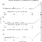
Figure 1: Monte Carlo (solid line) and analytic results (dashed line) for the velocity amplitude which, for a given fitted period, is exceeded by chance in 1% of analyses of simulated random data. A second solid line (histogram) shows the monte carlo results for the amplitude which is exceeded at any period within a range of approximately one octave, while the dotted histogram line shows the result from our analytic expression, eqn 15. For each of the experiments in the bottom two frames (5 and 20 obs./yr), the analytic and monte carlo results are indistinguishable. Assumed windowing at the lunar and annual periods as well as their double period counterparts are excluded from the monte carlo limits in their respective ranges.

For the subset of experiments with assumed 5 m/s precision, figure 1 shows the radial velocity amplitude for each fitted period which is exceeded in 1% of the Monte Carlo trials, ie. there is a 99% probability that a specific period analyzed will not exceed this value. Experiments with higher or lower assumed precision produce limits scaled upward or downward on the plot but otherwise show the same qualitative features. Also included are the $N=1$ limits provided directly by eqn. 13. In general, the Monte Carlo results confirm the validity of the analytical results above. The difference between $N=1$ analytic and Monte Carlo results varies about 2%, consistent with statistical fluctuations, except at the assumed windowing periods and at periods longer than $P_{0}$. The analytical prediction for the experiment with the most sparsely taken data (1 measurement per year for 12 years) lies some $\sim 15\%$ below the Monte Carlo result for periods less than 2 years, but agrees to $\sim 2\%$ over the remainder of the valid period regime.

A comparison of the limits provided by the analytical (eqn. 15) and Monte Carlo methods for each period range noted in Table 2 are also shown in figure 1. The assumed windowing periods are masked out of each of the Monte Carlo limits and the results represent limits based on the remaining portion of each range. In general, the Monte Carlo results again confirm the validity of the analytical result to within a few percent, with the exception of the series with only one measurement per year. In that case, the Monte Carlo experiment produces limits which are some 50% or more larger than eqn. 15 predicts.

We consider in turn in the sections below the differences between the analytical derivation and the Monte Carlo results due to the long period fall off in sensitivity, due to small numbers of observations, and due to the inherent windowing in the data.

3.2 Loss of Sensitivity at Long Periods

The results shown in figure 1 show that at periods longer than the 12 year window the sensitivity to a velocity signal drops off in very nearly power law form. In light of this behavior, we adapt an ad hoc prescription for the velocity limit using the eqn. 15 result at short periods and a power law at longer periods as

$$\hat{K}_{X}=\cases{K_{X}&for $P<\beta P_{0}$;\cr K_{X}\left({{P}\over{\beta P_{0}}}\right)^{\alpha}&for $P>\beta P_{0}$;\cr}.$$ (17)

We then fit for the free parameters $\alpha$ and $\beta$ and thereby recover limits for periods much longer than that of the observing window. In this equation, we assume that the value of $K_{X}$ used for long periods ($P>\beta P_{0}$) is that defined by the last period range prior to the onset of the fall off. This assumption ensures a smooth joining of the two regimes.

We fit the Monte Carlo results for the constants $\alpha$ and $\beta$ in eqn. 17 for each of the experiments and plot their values in figure 2 for both the six and twelve year observing windows studied. The fitted values for the 12 year window are typically:

$$\alpha\approx 1.86$$

with the turn off in sensitivity beginning between

$$1.4\leq\beta\leq 1.45$$

for the 99% probability curve and similar values for the 99.9% probability curve. A slightly steeper power law exponent ($\alpha\approx 1.92$) is found for a 6 year window. If we err on the side of caution and assume that the turn-off occurs at the small end of the range (by setting $\beta=1.3$, for both the 99% and 99.9% probabilities), then we provide slightly more conservative limits than the best possible based on our Monte Carlo analysis. Under this assumption, we have included in figure 1 the long period fits for the velocity limits placed upon the data by eqn. 17, and the shorter period limits for 11 period ranges less than $1.3\times$12 years.

3.3 Limits of Sparse Data

When a data set contains only a few measurements, a least squares analysis will depend strongly upon the measured value and placement in time of each measurement. How many data are needed to assure that the random data/random phase assumption is reliable and we are able reproduce the results of equations 13 (with $N$ set to unity) or 15 (for octave period ranges)? Is there a difference in the number of measurements that must be made if we assume a strategy of taking, say, one or two measurements per year over a long period or taking several measurements per year but over a much shorter baseline?

Taking the first strategy, we assume the data are gathered over a 6 year span with an error in each measurement of 5 m/s. If a star is observed with a frequency of one observation per year, we find (figure 3) that the eqn. 13 limits with $N=1$ underestimate the Monte Carlo results by more than a factor of two for periods shorter than 1 year, and by a smaller margin at all periods. The same experiment with a 12 year span shown in figure 1 shows a much smaller ($\sim$15%) difference. Increasing to three observations per year for 6 years the analytic equation underestimates the limits by $\sim$10%, while 5 measurements per year duplicates the analytic results to 5% or better.

For octave sized ranges, the analytical and Monte Carlo results converge somewhat more slowly. Figure 1 shows that a single measurement per year over 12 years is sufficient only to provide limits a factor of two higher than would be predicted analytically for periods less than 2 years. When data are gathered at the higher rates shown (5 and 20 obs/yr), the agreement is excellent. An experiment with two measurements per year (not shown), for a total of 24 measurements, is sufficient to recover the analytical form to $\sim$10% in all period bins. With the six year baseline shown in figure 3, agreement at the $\sim$20% level is reached if three measurements per year (18 total) are taken.

Taking the second strategy, we assume data are gathered over a two year window. We do not believe we can rely upon octave range limits for such a short data gathering period because of the large effects of windowing, which we discuss below. The long period fall off is similarly affected. We therefore limit our discussion for these experiments to limits for individual periods, shorter than about one year. With a two year data window and a total of 6 measurements (three measurements per year), we again find (figure 4) that the Monte Carlo limits exceed those of eqn. 13 with $N=1$ by more that a factor of two. Increasing to 6 measurements per year (12 total), we lose only 15% of the maximum sensitivity for $N=1$, while 12 measurements per year (24 total) recovers the analytic results with only a $\sim$5-7% difference.

In order to obtain limits which retain the benefits of a given precision to within 15% at any single period, we find that at least $\sim$12 or more observations of a star must be made. This number of observations produces limits a factor of two larger than predicted over octave ranges. To reduce the difference to $\sim$5% for a single period and 15% over octave ranges requires at least 18-20 measurements. Barring windowing effects, these minimum requirements do not seem to depend strongly upon the time span over which the data were gathered, but only upon their accuracy and number.

3.4 Windowing

Sensitivity loss of a factor of two or more is present in ‘blind spots’ for any single period near the assumed lunar and annual windowing periods for every experiment performed. There are also double period counterparts and beat periods between the lunar and annual data windows, though lower sensitivity loss is evident there. Day/night windowing effects are not visible in the limits due to their extreme short periodicities. When the data are sparse and the data are gathered over a short period $P_{0}$, the effects are especially pronounced. Figure 4) shows that for a period $P_{0}$ of two years, the lunar windowing effects are observable not only at the lunar orbital period, but also at the double, triple and quadruple period aliases. Additionally, fitting for the long period turn-off becomes of little use because the turn-off occurs at a period with lower sensitivity than can be modeled analytically.

Based on these results, we suggest that the limits which can be placed on signals at periods corresponding to a lunar or annual windowing period cannot be reduced beyond a factor of two greater than that given by eqn. 13 with $N$ set to unity at a windowing period or a factor of $\sim$3/2 at one of its double or beat period counterparts.

4 Comparison to Periodogram Techniques

To obtain definitive probability that a signal that been detected at some period is nonrandom, nothing less than a full Monte Carlo analysis is adequate. For a large survey which is continually updated as more data are gathered, such analysis is unfeasible because of the considerable commitment of computational facilities to perform a statistically meaningful analysis. Even for the computers of today, a sample of 500 stars might prove unmanageably burdensome. To reduce the effort required per star, either periodogram or fitting techniques such as ours may offer a lower cost alternative. We will now make a comparison of our technique to periodogram techniques in common use.

Each technique is based upon a $\chi^{2}$ analysis of the data. Indeed, for equally weighted data least squares analysis and periodogram analysis have been shown (Scargle 1982) to be equivalent. The main difference lies in the fact that on the one hand, a periodogram utilizes a normalized measure of the power of the signal at some period while our technique relies directly on the value of the best fit velocity amplitude. Additionally, with the present analysis, we allow the data to be fit with unequal weights, though the amplitude limits derived are based upon only upon equally weighted data.

Let us examine the least squares fitting procedure and, for purposes of illustration, limit ourselves to the case of fitting for only the coefficients $v_{s}$ and $v_{c}$ in eqn. 3. In this case, the best fit coefficients derived from the $\chi^{2}$ minimization at some frequency $\omega=2\pi/P$ for a set of $n_{0}$ velocity measurements, $v_{i}$, are:

$$v_{s}=C_{ss}\sum_{i=1}^{n_{0}}{{v(t_{i})\sin\omega t_{i}}\over{\sigma_{i}^{2}}}+C_{sc}\sum_{i=1}^{n_{0}}{{v(t_{i})\cos\omega t_{i}}\over{\sigma_{i}^{2}}}$$ (18)

and

$$v_{c}=C_{cs}\sum_{i=1}^{n_{0}}{{v(t_{i})\sin\omega t_{i}}\over{\sigma_{i}^{2}}}+C_{cc}\sum_{i=1}^{n_{0}}{{v(t_{i})\cos\omega t_{i}}\over{\sigma_{i}^{2}}}$$ (19)

where the subscripted $C$ terms are the four components of the covariance matrix used to derive the fit (see for example Press et al. 1992 ch. 15.4 for a discussion). When these terms are combined to form the velocity amplitude $K$ as $K=\sqrt{v_{s}^{2}+v_{c}^{2}}$ and data are translated in phase by a value $\tau=\tan^{-1}(v_{c}/v_{s})$ (derived by setting $C_{cs}=C_{sc}=0$) then, as was shown by Lomb (1976), the square of the best fit velocity amplitude, $K^{2}$, becomes the unnormalized power of the periodogram at that period. With the identification of $K^{2}$ with the periodogram power, we note that false alarm probabilities are given in each case is given as an exponential of $K^{2}$, with a normalization given by the variance, $\sigma^{2}$, of the data.

The use of the velocity amplitude rather than a normalized measure of its square represents an improvement to existing techniques for several reasons. First, a physically meaningful limiting velocity amplitude (or equivalently, a companion mass $\times\sin(i)$) is explicitly a part of the definition of the probability. A potential weakness of this method is that because it utilizes amplitude as a figure of merit rather than power, its dynamic range is more compressed on a given plot. A single dominant peak will not stand out to nearly the extent that occurs in a periodogram. In spite of this somewhat minor defect, we submit that a best fit amplitude is a far more useful quantity to an observer than is the power.

In sections 3.3-3.4 we have outlined the regimes for which our analysis is valid and the manner in which it fails for sparse or windowed data and for very long periods. Because of the similar origins of our analysis and periodograms we expect that similar failure modes also apply to periodograms. Hence probabilities derived from sparse data ($n_{0}\lesssim 10-15$) and at ‘windowed’ periods such as the annual cycle using a periodogram will yield erroneous results. Extensions to standard periodgram techniques (Irwin et al. 1989 and Walker et al. 1995) which explicitly account for unequal statistical weights and correlations between fit parameters may provide more accurate limits than our eqn. 15 in such regimes.

Our extensions to long periods explicitly provide limits on the amplitude of the signal (and therefore $M\sin(i)$) possible at any given period at least 10 times as long as the data window. The limits account for the fact that a long period signal may in fact be near an extremum during the time over which most or all of the data were gathered.

Both techniques may be used to determine the probability of a signal being nonrandom for a single period, for a period range or over all independent periods. The Scargle (1982) and HB false alarm probability generates the probabilities, in the ideal case, by requiring a Monte Carlo analysis to specify the number of independent periods, $N$. Their analysis to determine $N$ is limited to sampling frequencies below the Nyquist limit however. With unevenly sampled data, it is well known that higher frequencies are accessible without aliasing. How far above the Nyquist limit a signal can be detected and how many additional independent frequencies (if any) are required remains unknown.

We also require a specification of the number of independent periods, however our analysis uses a definition of the number of independent periods (not equivalent to the HB definition) based only upon the width of a spectral peak. We make no distinction between potentially aliased spectral peaks at high frequencies and those found at lower frequencies. The excellent correspondence between our analytical formalism and our Monte Carlo analysis for each period range shows that the definition of $N$ made in eqn. 14 is reasonable. The functional dependence of the amplitude limit on $N$ is quite weak, going only as $\sqrt{\ln{N}}$. When $N$ is large, as is the case for the shortest period bins, our definition will yield slightly more conservative (higher) limits than the comparable HB limits, while for longer periods when $N\lesssim 100$, our limits may be somewhat lower.

5 Application to Real Data

In this section we apply our analysis technique to data for two stars obtained by Mayor and his collaborators at the Geneva Observatory, data obtained by Marcy et al. (1997) for the star 51 Pegasi, and to the data obtained by Walker et al. (1995) in their 12 year search for extra-solar planets. The Walker et al. radial velocity data are for a set of 21 stars with data taken over a 12 year period from 1980-1992. The data used in our analysis were originally archived at the Astronomical Data Center (URL http://hypatia.gsfc.nasa.gov/adc.html) by Walker et al. upon publication of their work. We limit our analysis to the subset of 14 stars for which no visual binary companion is known, shown in Table 1. For these stars, no other periodic radial velocity signatures which could obscure a planetary signature are present, and no significant periodicities attributable to planetary companions were found by the Walker et al. search.

Using equations 4 and 15 we can derive for any period (or period range) of interest the limit below which random data is fit with probability $X$ to be:

$$M_{c}={{{\hat{K}_{X}}\over{\sin(i)}}\left({{PM_{*}^{2}}\over{2\pi G}}\right)^{1/3}}$$ (20)

where we assume the orbital period, $P$, is at the midpoint of some range of periods shorter than $\beta{P_{0}}$ or that $P>\beta{P_{0}}$. This mass limit depends upon both the velocity amplitude limit $K_{X}$, which changes slowly, and also the period for which we fit the data. The minimum mass detectable by a set of measurements increases only as the cube root of the period at short periods, but for $P>\beta{P_{0}}$, this dependence becomes much steeper, increasing faster than $P^{2}$.

Once we have mass or velocity amplitude limits for a set of data, we can define quantities $M_{99}$ and $M_{999}$ via eqn. 20 as the mass exceeded by chance by a fit at the 1% and .1% level of probability in each period range. For a sample of radial velocity measurements of say 10 stars observed for 10 years divided up into 10 period ranges, these values are of interest because if there are no true periodicities in the data, we would expect to find by chance one apparent planet with best fit mass $M>M_{99}$, but to find a mass greater than $M_{999}$ with only $\sim$10% probability.

5.1 Determining the Measurement Uncertainty

In order to obtain a value of $\sigma_{p}$ for use in eqn. 15 or 20, we assume that no strong periodic signals are present in the data and that each datum is drawn from the same statistical distribution. Then we may use the rms scatter of all the data for a star as an empirical measure of the error, $\sigma_{p}$, for each measurement of that star. For data in which no clear signal is observable, this measurement of the error will give a more reliable estimate of the true value than from internal estimates. In Table 1, we show both $\sigma_{p}$ as derived directly from the data as well as the average of the internal errors for each star ($\sigma_{i}$) quoted by Walker et al.

5.2 Detecting Large Amplitude and Large Eccentricity Signals

In this section we show that our analytic technique is capable of detecting large amplitude signals and signals with high eccentricity. As an initial test we obtained the data for the original discovery of the companion to 51 Pegasi, taken by Mayor and his collaborators at the Geneva Observatory. These data consist of the original 35 measurements as published by Mayor and Queloz (1995) as well as their observations of the star since that time. The total number of observations used in our analysis was 89 radial velocity measurements made over 2.4 years with internal errors of 15 m/s. The value for $\sigma_{p}$ was obtained from the rms scatter of all of the velocity measurements and was $\sigma_{p}=44.5$ m/s. An independent set of measurements (Marcy et al. 1997) was also used to compare the technique using higher precision data. A total of 116 measurements are characterized by an rms scatter of $\sigma_{p}$=40.6 m/s and were gathered over a total time span of 325 days with internal errors of 5 m/s.

We show the results of these two tests in figure 5. For each set of measurements, we detect a clear peak in the best fit velocity amplitude at a period $P=4.23$ days, as expected. For the Mayor and Queloz data, we also detect a number of side lobes peaks which represent the radial velocity signal ‘beating’ against other periodicities in the data such as the 29.5 day lunar cycle (the data were taken predominantly during the same half of each lunar cycle). The Marcy et al. data show one 99% significant peak just shortward of one year. We consider this peak to be an artifact of the short time baseline of their data (less than one year) and do not consider it very significant.

A second 99% significant period is detected at 23.84 days in the Mayor and Queloz data. We have re-analyzed the residuals of the measurements (with the 4.23 day periodicity removed) and found that the peak remains and so cannot be attributed to an alias of 4.23 day periodicity. Is it an artifact of the rotational period of the star itself? We note that the period is roughly in a 2:3 ratio to the observed 37 day rotation period for 51 Peg (Henry et al. 1996). We suspect that with the incomplete phase coverage for periods near 24 and 37 days, the stellar rotation period may be aliased to the observed 23.84 day period. Only complete phase coverage may be able to determine the origin of this signal.

The independent radial velocity observations of Marcy et al. do not show a similar periodicity and the precision of their measurements is only half the best fit amplitude from the Geneva data. In their work more than 3/4 of the data were gathered in less than two rotation periods of the star. In such a case, it is unclear whether a rotation signature would be observable in Doppler spectroscopy data.

As a second test, we obtained another set of radial velocity data from Mayor. In this case the data were obtained under the condition that the identity of the data and whether they contained a signal not be disclosed until the conclusion of the test. These data consisted of 45 measurements taken with the CORAVEL spectrometer with internal errors of 300 m/s. The data were gathered over $\sim$15 years and the value for $\sigma_{p}$ obtained from the rms scatter in the velocity measurements and was $\sigma_{p}=800$ m/s.

The best fit velocities and the corresponding 99 and 99.9% probability limits for the fits are shown in figure 6. In this case, we were unable to detect a significant periodicity in the data except a possible long term signal near 15 yr. The data show no obvious periodicity in the velocities for orbits of $\sim$15 yr, but do show that several measurements are some 3–5 $\sigma$ away from the mean of any other velocity measurements of the star. These data were gathered within 6 days of each other in the fall of 1996.

To test the effect of these data we deleted them from the sample and reapplied our analysis. In this case, the rms scatter was reduced to $\sigma_{p}=480$ m/s and $n_{0}$ to 40 while the duration of the measurements $P_{0}$ remained the same. Figure 7 shows the results of this reanalysis. In this case a peak in the best fits for a circular orbit, well above the 99.9% probability curve, becomes visible at 275 days. With the detection of this peak, we concluded our test and obtained the identity of the star from which the observations were taken. The star from which the data were obtained was HD 110833, for which Mayor et al. (1996) published an orbital solution with a best fit companion mass $M\sin(i)=17~{}M_{J}$, a period of $P=270$ days and an orbital eccentricity $e=0.7$ using data from both the CORAVEL and ELODIE spectrometers. The difference in the period derived from our analysis and the Mayor et al. fit is due to the inconsistency between the high eccentricity of the companion and assumption made in our analysis that the orbit is circular.

In discussions with M. Mayor and D. Queloz, several issues were brought forward. First, the data from the fall 1996 run may have been faulty due to a combination of several factors, including a slight misfocusing of the telescope or a temperature instability in the spectrometer itself. However, while the measurements in question are unusually distant from the mean of the other measurements for that star, they were gathered during a single periastron passage of the companion and therefore may not contribute as strongly to the detection of the periodicity as they would otherwise. A fit for the set of orbital elements would then yield a higher eccentricity than is truly the case.

This case may therefore expose a degeneracy between results using data derived from a companion which is truly in a highly eccentric orbit and data with possible systematic biases. Our technique is based upon only the lowest order Fourier components of the signal (i.e. a circular orbit) and does not account for eccentric motion. The fact that so many data (5 of 45 measurements) were so far from the mean and that they were from the same observing run suggests that removing the data from that run from our analysis is justified. Omitting them, we are able to recover a strong periodicity near the best fit period for the orbital solution.

With the results from this section we can be confident that our analytic technique is capable of detecting signals with large amplitude and/or large eccentricity.

5.3 Masses from Best Fit Velocities of the Walker et al. Sample, and Analysis of Significance

We have shown that our analytic technique is capable of detecting large amplitude periodicities in radial velocity data. In this section we move to lower amplitude signals and upper limits to companion signatures. For each star in the Walker et al. sample, best fit velocities for periods between 3 days and 100 years were determined by the least squares method using eqn. 3. Statistical weights for each datum were taken to be 1/$\sigma_{i}^{2}$, where $\sigma_{i}$ is the quoted internal error for each point s as given by Walker et al. Plotted in figure 8 are the corresponding companion masses $M_{c}\sin(i)$ obtained from eqn. 4 using the stellar masses from table 1. In order to determine the significance of any particular best fit value we compare the best fit mass for some period to the limit provided by our analytical analysis and to Monte Carlo experiments similar to those described in section 3 for synthetic data. Each of these limits are shown in figure 8.

While as expected from the results of the original analysis of Walker et al., there are no clear cut companion signatures, in several cases the data produce statistically significant fits. We tabulate each of these periods in table 3. Are any of these signatures due to the existence of a companion? Stellar processes such as pulsation, rotation or magnetic cycles can affect the measured radial velocity for a star and in many cases it is quite possible to fit such signals with orbital solutions. Early in this century for example (see eg. Jacobsen 1925, 1929), the radial velocity variations of Cepheid variable stars were fit with Keplerian orbits. Although today no one would attribute Cepheid radial velocity variations to a companion, the principle that processes intrinsic to the star must be eliminated from consideration remains if we are to be certain that a given radial velocity detection is definitely due to a companion.

Many of the signals in table 3 do in fact correlate with known periodicities due to stellar rotation or magnetic cycles in the star. For example, we find a $>$99.9% significant $\sim$10 yr period in $\epsilon$ Eri and two short period signals (at 11.9 and 52.5 days) with $>$99% probability. Walker et al. establish that the 10 year and 52 day peaks are aliases of each other and McMillan et al. 1996 have definitely connected this periodicity to a stellar magnetic cycle. Gray and Baliunas (1995) have observed an 11.1 day periodicity in the Ca H&K S-index with an extensive data set. They comment that subsets of their data taken during different observing seasons produce peaks varying in period from 11 to 20 days. We conclude that we are seeing a comparable effect in the Walker et al. radial velocity data and are in fact detecting the rotational signature of the star.

Further work by the same group (Gray et al. 1996) on the star $\beta$ Com provides evidence of a magnetic cycle. However their measurements have sufficient duration only to have observed a minimum, and a period is not known. Figure 8 shows that for $\beta$ Com the probability that the best fit velocity amplitude is not random exceeds 99% for periods near 10 years. Assuming a 10 year period, we calculate that the best fit radial velocity curve went through its minimum in 1988/1989, which is coincident with the photometric and Ca H&K minimum observed by Gray et al. (1996). Significantly, the radial velocity minimum is not coincident with the velocity span minimum derived from their line bisector analysis.

The star $\eta$ Cep shows $>$99% significant periodicities at $P=$164 days and $\sim$10 yrs. Walker et al. have speculated that the 164 day periodicity was due to stellar rotation. No periodicities are detected in line asymmetry to $\sim$19 m/s by Gray (1994) with measurements spanning four years. However we find the best fit radial velocity amplitude at each of these periods is only 16 and 13 m/s respectively. If a direct correlation between a radial velocity measurement and a line bisector measurement exists, such signals would be below his detection limit. By analogue with $\epsilon$ Eri, we speculate that the 10 year periodicity in $\eta$ Cep might be linked to a magnetic cycle, but we cannot be certain of its origin.

Other marginal periodicities appear in the data for HR 8832 and $\theta$ UMa. Again by analogue with other stars, in this case $\epsilon$ Eri and $\eta$ Cep, we might speculate that these shorter periodicities are due to stellar rotation, however no certainty can be attached to their origin.

We also find that two stars in the subset (36 UMa and $\beta$ Vir) show best fit minimum masses which, for fitted periods longer than $\sim$12 years, rise above the curve for which the best fits are random with 99% and 99.9% probability. Walker et al. find similar trends in these stars but make no firm conclusions based upon their analysis. Are these signals indications of long period companions, or are they also due to stellar effects? We show the data for these stars in figure 12, both raw and binned by year. While the raw data show no obvious signals, the binned data, particularly for 36 UMa, show some indication of a partially complete sinusoid. We note that in both cases, the curvature in the velocity trends is of the same sign and the portion of the sinusoid is similar, which suggests a long term calibration error. However, the binned data for all stars taken together shows no such trend so a systematic explanation seems less likely.

5.4 A Check by Monte Carlo Analysis

Each of the stars in the Walker et al. sample average 3-5 measurements per year over the 12 year period and, according to the results of section 3.3, this number should be sufficient for application of our analytic apparatus. We note however, that implicit in our analytical derivation of mass limits is the assumption that the measurements be at least somewhat regularly distributed. In the case of the Walker et al. data, this is not always the case. The data are irregular on both short time scales (ie. 3 night runs consisting of 1–3 velocity measurements per star per run) and longer time scales, for which more data may be loosely clustered on several year time scales due to changes in observing procedures etc. Because of these irregular sampling patterns fits may be less tightly constrained than a more evenly spaced data set, and the limits provided by our analytic apparatus may become misleading.

Since the Walker et al. data are rather irregular, we examine the effect on our analysis technique by performing a Monte Carlo experiment and comparing the result to our analytic formalism. We create synthetic data sets using a constant value of the error, $\sigma_{p}$, equal to the rms scatter of the observed velocity measurements for each star. This value is input into eqn. 16 to derive individual simulated velocity measurements. We use the observation times given by the data itself. We fit the measurements and derive best fit velocity amplitudes (and corresponding $M_{c}\sin(i)$ values) for periods between 3 days and 100 years Each synthetic datum used in the fit is weighted with the internal error in that point (quoted by Walker et al.) as $1/\sigma_{i}(t_{i})^{2}$.

The results of these experiments are shown as the solid histograms in figure 8. In general, the agreement between the analytic limits and the Monte Carlo experiments is good. However a small systematic trend towards larger limits for the Monte Carlo experiments is found. Typically the difference is 10% or less, however, in the most extreme case ($\theta$ UMa), the limits produced are about 20-30% higher than with the analytic method. This star has the shortest time baseline of any in the sample as well as one of the largest degrees of clumping of any star in the sample, as measured by the ratio of the number of data to the number of runs. A test in which we replace in eqn. 17 the number of data, $n_{0}$ with the number of runs recovers the Monte Carlo results for this star quite well. The star $\epsilon$ Eri, for which the data are the most highly clumped of any star in the sample, also produces analytic limits lower than reproduced with the Monte Carlo experiment. In this case, replacing $n_{0}$ with the number of runs produces limits much larger than the Monte Carlo result, so we cannot recommend such a procedure for general use.

In the case of one star (HR 8832), two measurements were made with a 3-1/2 year separation from any other measurement for that star. This case provides an interesting test in the limit of very irregularly spaced data. We find that the limits derived from the Monte Carlo experiment are quite similar to the analytic result except in the range between about 8 and 12 years, where limits some 20% larger than those derived via eqn. 20 are found. The longer period fall-off characteristics are unaffected by the irregularity.

The sensitivity fall off at long periods for each star is similar to that produced in the synthetic data. We show the derived fit values for the power law exponent and the long period turn off in figure 11 for the sample of 14 stars. The sharp upturn in limiting velocity at long periods produces a power law exponent which is best fit with values near $\alpha=1.86$, while the turn-off period, $\beta$, is best fit with values near $\beta=1.45$, but with a larger scatter than is present in the synthetic data. Because the scatter is by its nature rather unpredictable from star to star, we retain the low $\beta=1.3$ value found for synthetic data when determining limits via eqn. 17 or 20.

The limits provided by our analytic expression produce upper bounds which are ordinarily $\lesssim$10% different than those produced via Monte Carlo experiments. In the most irregularly spaced data, a difference of up to 20-30% can occasionally be produced. In several cases, the difference results in possibly spurious ‘detections’ of marginal signals by the analytic technique where the Monte Carlo limits do not show that the periodicities are significant. In some of these cases we are able to attribute the detections to physical processes discussed in the literature. In no case do the analytic limits exceed the 99.9% level of probability where the Monte Carlo result did not also show at least a 99% probability. Despite this level of difference, our conclusions about the significance or lack of it for any periods and companion masses for each star in the Walker et al. data remain unchanged. We are confident that this method can be relied upon to obtain probabilities that a given set of data contains a periodic signal.

5.5 Sensitivity to Short Period Planets

For the star with the lowest companion mass limits ($\epsilon$ Eri), we have also plotted in figure 8 several recent planet detections (Mayor and Queloz 1995, Marcy and Butler 1996, Butler and Marcy 1996, Latham et al. 1989, Gatewood 1996, Noyes et al. 1997) and Jupiter. Extra solar planets with combinations of period and mass like those shown would have been readily detected by Walker’s radial velocity measurements. These stars do not have such companions. For most of the stars in the sample, the data are too noisy to have reliably detected a radial velocity signature such as would be predicted for the companion to Lalande 21185, announced by Gatewood (1996) but which remains unconfirmed. Planets such as Jupiter, which would appear at $P=12$ years with a typical value of $M_{c}\sin(i)$=0.64$M_{J}$ would not have been reliably detected. The best fit values exceed this period/mass combination in 40% of the sample.

The analysis of Walker et al. sets upper limits to the mass of companions in their sample ($\times\sin(i)$) of $\leq 1M_{J}$ and $\leq 3M_{J}$ in periods of less than 1 year and 15 years respectively. In general, our analysis provides limits which are somewhat lower than theirs in both long and short period orbits. For one year periods, we can limit companion $M\sin(i)$ values to $\leq 0.7M_{J}$ for all but three stars in our subset and $\leq 1.0M_{J}$ for the rest. In 15 year orbits, our analysis limits possible $M\sin(i)$ values to $\leq 1.5M_{J}$ for every star except $\theta$ UMa, for which only 6 years of data were gathered. For this star, the limit is $\leq 4.0M_{J}$. We have also extended range over which companion signatures are constrained to shorter periods than were analyzed in Walker et al. The limits for these extreme short period orbits ($P<40$ days) correspond to companion masses ($\times\sin(i)$) below 0.4 $M_{J}\sin(i)$.

Under either our own analysis or the original analysis of Walker et al., the companion mass limits derived from the data essentially eliminate brown dwarfs and large Jovian planets with periods $\lesssim 15$ years, barring very unfortunate inclinations. Given the detections of significant periodicities by either our analytic treatment or Monte Carlo experiments, we find more signals present than can be attributed to purely random data. In some cases, such detections may be due to physical mechanisms other than a companion, and we have compared these to known periodicities due to stellar rotation or magnetic cycles, where they have been identified in the literature. In no case do the limits eliminate the possibility of gas giants such as exist in our solar system or low mass brown dwarfs, especially in the period/radius range $\geq$12 yr/5 AU where theory predicts such companions.

6 Strategies for Large Radial Velocity Surveys

There are currently six active groups with programs for radial velocity searches at the $<$10-20 m/s level. Three groups began searches at this precision in 1987-88 (Cochran & Hatzes 1994 (Texas), McMillan et al. 1994 (Arizona), Marcy & Butler 1992 (Lick)), while one (Duquennoy & Mayor 1991 (Geneva)) have used lower precision measurements with the CORAVEL spectrometer ($\sim 300$ m/s) to investigate stellar binary companions and have recently built a new spectrometer (ELODIE) to allow $\lesssim$15 m/s precision measurements to be made. The latest high precision searches (Kürstner et al. 1994 (ESO), Brown et al. 1994 (CfA)) began in 1992 and 1995 with quoted precision of $\sim$4-7 m/s and $\sim$10 m/s respectively. Another group (Walker et al. 1995 (UBC)) concluded a 12 year search in 1992. Two others (Mazeh et al. 1996 (CfA), Murdoch et al. 1993 (Mt John NZ)) obtain precision of $\sim$500 m/s and $\sim$60 m/s respectively.

The recent discoveries of sub-stellar mass companions around other stars have stirred new interest in very large radial velocity surveys. The Geneva group for example, intends to expand their search to $\sim$500 stars in the northern hemisphere (ELODIE) and another $\sim$800 in the southern hemisphere (CORALIE), and other groups have similar expansions underway. In order to observe as many stars as possible with a finite telescope allocation, such large surveys must necessarily aim toward the most efficient use of the available observing time. The goal of such large surveys might be properly stated as “What fraction of stars have a companion (or a system of companions) and what is the distribution of the masses, periods and eccentricities of those companions?”.

In order to answer this question three criteria must be met. First, an observer must first detect a variation in the radial velocities measured for a star about which a prospective companion orbits. Second, the observer must determine the origin of such variations by fitting a Keplerian orbit and by making additional photometric or spectroscopic observations to constrain effects due to the stellar photosphere. Finally the observer must determine the extent to which the survey is complete: what fraction of stars which were observed may have companion signatures which went undetected over the course of the survey? Based on the analysis in this paper, we can suggest strategies for the most efficient methods of detecting radial velocity signatures and which also provide meaningful upper limits on the amplitudes of undetected signatures.

Let us suppose that the random error for each measurement is dominated by photon noise, ie. that $\sigma_{p}\propto 1/\sqrt{t}$, where $t$ is the length of a single observation. This should be the case provided detector read noise is not significant. It follows from eqn. 15 that the limiting amplitude, $K$, is proportional to $1/\sqrt{t_{n}}$, ie. $K$ depends on the total integration time devoted to a star, $t_{n}$, independent of number of observations making up that time. In other words, as long as eqn. 15 holds and the total integration time is the same, making many lower precision measurements is equivalent to making fewer high precision measurements. Since constraining additional orbit parameters such as eccentricity is at its most simplistic level an exercise in detecting higher order Fourier components of the signal, this equivalence holds for orbit determinations as well as for detection of a periodic signal. We caution, however that with lower precision data, larger amplitude systematic errors may go undetected. With 15 m/s precision for example, the signal of Jupiter could be completely obscured by a hidden systematic error of amplitude $\sim$10 m/s.

From section 3, to insure than eqn. 15 holds, the number of observations, $n_{0}$, must be at least $\sim$12 and preferably as high as 20 in order to constrain octave period ranges. The limits are degraded most severely for periods less than 1–2 years. Longer periods limits are nearly identical to the analytic prediction even for very sparse data (see figures 1 and 3). This is because with only a few observations of each star, a companion signature could still slip through undetected if by some unfortunate coincidence its radial velocity “zero crossings” corresponded to the times at which the star was observed. For $P\lesssim 1$ year, there are very many independent periods, so that the possibility of any one of them coincidentally undergoing such a zero crossing event is very high. For $P\gtrsim 1$ year, where there are relatively few independent periods, such a condition becomes much more unlikely.

The cost in observing time to obtain useful limits if there are few observations is great. When the data are sparse and eqn. 15 breaks down, for example with a total of either $n_{0}=6$ or $n_{0}=12$ observations and the same total integration time, our Monte Carlo simulations show that the limiting amplitude is in fact twice as big for any single period, and ten times as big for octave period ranges. Because 12 much lower precision measurements would identically constrain short period signals as 6 high precision measurements, the increase in sensitivity translates to a reduction factor of 4 or 100 in the amount of observing time required to identically constrain the existence of companion for any single period or over octave ranges in orbits of $\lesssim 2$ years.

As an example of a strategy which addresses this concern, suppose a survey is to observe 500 stars and is to last at least 12 years. Let us also suppose that 1/4 of the use of a telescope is dedicated to the radial velocity measurements, yielding about 400 hours of integration per year to be divided among the stars in the survey. The total number of observations to obtain 12 for each star is 6000. A good “quick look” could be obtained after the first two years if each observations takes 2$\times$400/6000 hours = 8 minutes.

Butler et al. (1996) report that precision of $\sim$3 m/s can be obtained in a 10 minute exposure of a magnitude $V=5$ star on a 3 meter class telescope. However, in a large survey most stars will be dimmer than $V=5$, with a practical limiting magnitude between $V=7$ and $V=8$, depending on the size of the survey. If the average star is of magnitude $V=7$, a measurement with 3 m/s precision would nominally require about 60 minutes. With such long duration measurements each star in the program would average less than one observation per year and would make a large, high precision survey unfeasible. In order to complete a large survey at $\leq$5 m/s precision a large allocation of time on an 8–10 m class telescope would be required. If instead we allow reduced precision measurements of $\pm$10 m/s, using our assumption that the precision is proportional to $1/\sqrt{t}$, a single measurement would require only about 6 minutes on a 3 meter telescope, which would be feasible for a large survey.

For this to be practical without poor observing efficiency, the time from the end of an observation to the beginning of the next on a new star must be short, ideally a minute or less. During this time, the telescope must be slewed to the new star, while the CCD with the exposed spectrum is read out. Automatic slewing and acquisition would make this quite practical. Also, for a typical spectroscopic CCD with around 3 million pixels, the required read rate of 100 kpixel/sec should be readily achievable at negligible read noise with current devices. A 8 minute cycle time with 6 minutes data acquisition would thus be a reasonable target, and yield 72 minutes of integration for each star, spread through the first two observing seasons.

With this strategy, an observing program should be able to sustain 6 measurements of every star every year that the program is continued. If after two years, variations are detected in some stars, additional measurements of those stars would be possible if constant velocity stars were observed only 1–3 times per year. This compromise has the advantage that limits on companion masses are well constrained by such density of points and orbital solutions, should a star’s velocity later be observed to vary, would also be well constrained. A second advantage is that after the first two years, strong limits on the existence of a companion signal are available for short periods and these limits extend to longer periods incrementally as long as the program is maintained. In contrast, a high precision/sparse observation strategy with say 1-2 measurements per year, will strongly limit short period signatures only after 6 or more years of the program has passed.

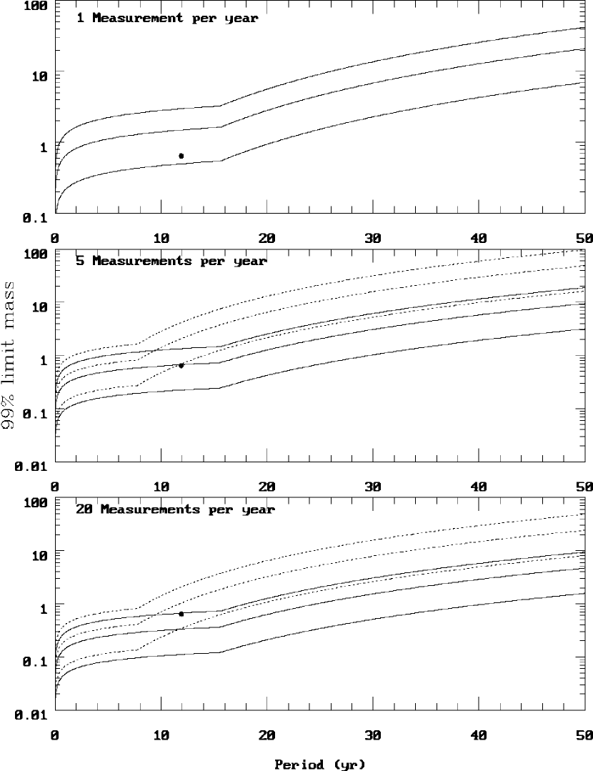
Figure 14: Limits above which data of a given quality and duration constrain the mass of companions at the 99% level for any single period. Solid lines represent a 12 year span of data taken with 5, 15 and 30 m/s precision while dotted lines represent a comparable 6 year span. Limits for the 6 year baseline with one only measurement per year are omitted here because they do not correspond to results from monte carlo experiments (see section 3.3).

As a second example of observing strategy, we consider a search for a Jupiter mass planet with the same 12 year period as Jupiter, around a star with the same mass as the sun, what accuracy measurements are needed over what period to ensure only 1% probability of a false detection for any given star? For sets of observations spanning 6 and 12 years figure 14 shows the limiting mass above which a companion would be detected with 99% probability in a given set of data at any single period. A 1 $M_{J}$ companion in a 12 year orbit around a solar twin will have a best fit mass of $\sim 0.64M_{J}$ assuming a random inclination. We require via eqn. 20, that data be taken with precision $\pm$5 m/s for 12 years with a single observation per year in order to detect such a companion. Increasing to 5 or 20 observations per year, only 15 or 30 m/s are required, respectively, with the requirement that no hidden systematic errors are also present in the data. For an identical number of measurements per year, a 6 year baseline requires more than 6 times the precision in each measurement to similarly constrain a long period companion, or 36 times the observing time each year. Clearly the cost of impatience is very high.

Table 1: The Subset of 14 Stars Included in our Analysis

HR	HD	Name	M/M⊙	$\sigma_{i}$	$\sigma_{p}$	Number	Number	Duration
				(m/s)	(m/s)	Obs.	Runs	(yr)
509	10700	$\tau$ Cet	0.87	13	17	68	39	11.7
937	19373	$\iota$ Per	1.15	15	18	46	29	10.8
996	20630	$\kappa^{1}$ Cet	0.98	13	20	34	22	10.0
1084	22049	$\epsilon$ Eri	0.82	14	16	65	34	11.1
1325	26965	o2 Eri	0.84	14	19	42	28	11.0
3775	82328	$\theta$ UMa	1.45	24	21	43	23	06.0
4112	90839	36 UMa	1.08	16	21	56	36	10.7
4540	102870	$\beta$ Vir	1.22	14	26	74	48	11.7
4983	114710	$\beta$ Com	1.09	16	18	57	40	11.4
5019	115617	61 Vir	0.98	13	18	53	35	11.4
7462	185144	$\sigma$ Dra	0.85	13	19	56	37	11.5
7602	188512	$\beta$ Aql	1.30	12	14	59	39	11.4
7957	198149	$\eta$ Cep	1.36	12	19	58	39	11.2
8832	219134	$\cdots$	0.79	11	15	32	23	10.6

Table 2: Period Ranges

3-6d

6-12d

12-24d

24-48d

48-96d

96d-0.5yr

0.5-1yr

1-2 yr

2-4 yr

4-8 yr

8-12 yr

$>$12 yr

Table 3: Detection of Significant Periodicities

Period range	Star	Period	Companion	Probability of Chance
			Mass (MJ)	Detection in Period Range
				Analytic	Monte Carlo
3-6d	$\cdots$
6-12d	$\epsilon$ Eri	11.9d	0.14	$<$1%	$\cdots$
12-24d	$\cdots$
24-48d	$\cdots$
48-96d	$\epsilon$ Eri	52.5d	0.24	$<$1%	$\cdots$
96d-0.5yr	$\eta$ Cep	164d	0.54	$<$0.1%	$<$1%
	HR 8832	165d	0.35	$<$1%	$\cdots$
	$\theta$ UMa	179d	0.63	$<$1%	$\cdots$
0.5-1yr	$\cdots$
1-2 yr	$\cdots$
2-4 yr	$\cdots$
4-8 yr	$\epsilon$ Eri	$>$7 yr	0.70	$<$1%	$<$1%
8-12 yr	$\epsilon$ Eri	10 yr	0.95	$<$0.1%	$<$1%
	$\eta$ Cep	10 yr	1.20	$<$1%	$<$1%
	$\beta$ Com	10 yr	1.05	$<$1%	$\cdots$
	36 UMa	10 yr	1.10	$<$0.1%	$<$0.1%
$>$12 yr	36 UMa	15 yr	2.00	$<$0.1%	$<$0.1%
		25 yr	5.30	$<$0.1%	$<$0.1%
		50 yr	24.00	$<$0.1%	$<$0.1%
	$\beta$ Vir	15 yr	1.90	$<$0.1%	$<$0.1%
		25 yr	5.00	$<$0.1%	$<$1%
		50 yr	23.00	$<$1%	$<$1%

Figure 2: Best fit values for the long period sensitivity fall off parameters $\alpha$ and $\beta$ for the nine monte carlo experiments run for both 6 and 12 year baselines.

Figure 3: Velocity limits given by monte carlo simulations (solid), single period ($N$=1) analytic limits (dashed). The histograms represent the monte carlo (solid) and analytic (dotted) limits for octave sized ranges. Each of the histogram limits ignore the periods affected by the assumed lunar and annual windowing of the data. A 6 year window is assumed with 1 (top), 3 (middle) and 5 (lower) observations per year.

Figure 4: Velocity limits given by monte carlo simulations (solid), single period ($N$=1) analytic limits (dashed). A 2 year window is assumed with 3 (top), 6 (middle) and 12 (lower) observations per year. As before, histograms represent the monte carlo (solid) and analytic (dotted) limits for octave sized ranges and each of the histogram limits ignore the periods affected by the assumed lunar and annual windowing of the data. In this plot however, for periods longer than 1 year the monte carlo histogram limits are suppressed.

Figure 5: Best fit velocities for the star 51 Pegasi. The solid and dotted histograms denote respectively, the limits below which random data would occur with 99 and 99.9% probability.

Figure 6: Best fit velocities for the data derived from star HD 110833. A 15 year periodicity is apparent in the best fits with $>$99% probability that it is nonrandom.

Figure 7: Best fit velocities for the the subset of the data from HD 110833 with 5 measurements removed. In this case, a periodicity is present at 275 days with probabability $>$99.9% that it is non-random.

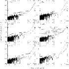
Figure 8: Best fit companion masses ($\times\sin(i)$) for each star over a range of periods corresponding to the most sensitive range of the data. The histograms represent the 99% mass limits for each specified period range as given by our analytic formulation (dotted histogram) and based on a monte carlo experiment (solid histogram) consisting of 3000 simulated data sets. Also plotted (squares) are the measured $M_{c}\sin(i)$ values of recent planet detections (see text). Jupiter and the astrometrically detected (but unconfirmed) companion to Lalande 21185, are shown omitting a $\sin(i)$ correction (circles).

Figure 8–cont:

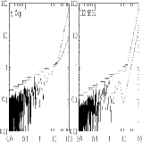
Figure 8–cont:

Figure 11: Best fit values for the long period sensitivity fall off parameters $\alpha$ and $\beta$ derived from the data. Values for both 99% (triangles) and 99.9% ($\times$’s) fall-off are shown. The two points lying to the right of the main group originate from the star $\theta$ UMa and are consistent with the monte carlo results for a 6 year data span.

Figure 12: Radial velocity data for the stars (a) 36 UMa and (b) $\beta$ Vir, for which long term trends are observed using both our analysis technique and the Walker et al. analysis. Both the published velocity data and the weighted mean of the velocities for each year are shown. The binned data for the sample of 14 stars taken together is shown offset by $-50$ m/s. No trend similar to that found in either 36 UMa or $\beta$ Vir is present, indicating that a systematic error common to all stars is unlikely. Errors are taken from Walker et al. 1995, while the errors in the binned points are derived from the central limit theorem 1/$\sqrt{n}$ improvement in the error of a multiply sampled mean.

Figure 12b: