Dynamics of Circumstellar Disks
Abstract
We present a series of 2-dimensional hydrodynamic simulations of massive disks around protostars. We simulate the same physical problem using both a ‘Piecewise Parabolic Method’ (PPM) code and a ‘Smoothed Particle Hydrodynamic’ (SPH) code, and analyze their differences.
The disks studied here range in mass from to and in initial minimum Toomre value from to . We adopt simple power laws for the initial density and temperature in the disk with an isothermal () equation of state. The disks are locally isothermal. We allow the central star to move freely in response to growing perturbations. The simulations using each code are compared to discover differences due to error in the methods used. For this problem, the strengths of the codes overlap only in a limited fashion, but similarities exist in their predictions, including spiral arm pattern speeds and morphological features. Our results represent limiting cases (i.e. systems evolved isothermally) rather than true physical systems.
Disks become active from the inner regions outward. From the earliest times, their evolution is a strongly dynamic process rather than a smooth progression toward eventual nonlinear behavior. Processes that occur in both the extreme inner and outer radial regions affect the growth of instabilities over the entire disk. Effects important for the global morphology of the system can originate at quite small distances from the star. We calculate approximate growth rates for the spiral patterns; the one-armed () spiral arm is not the fastest growing pattern of most disks. Nonetheless, it plays a significant role due to factors which can excite it more quickly than other patterns. A marked change in the character of spiral structure occurs with varying disk mass. Low mass disks form filimentary spiral structures with many arms while high mass disks form grand design spiral structures with few arms.
In our SPH simulations, disks with initial minimum or lower break up into proto-binary or proto-planetary clumps. However, these simulations cannot follow the physics important for the flow and must be terminated before the system has completely evolved. At their termination, PPM simulations with similar initial conditions show uneven mass distributions within spiral arms, suggesting that clumping behavior might result if they were carried further. Simulations of tori, for which SPH and PPM are directly comparable, do show clumping in both codes. Concern that the point-like nature of SPH exaggerates clumping, that our representation of the gravitational potential in PPM is too coarse, and that our physics assumptions are too simple, suggest caution in interpretation of the clumping in both the disk and torus simulations.
1 Introduction
Over the past several years a broad paradigm of star formation has been developed (see Shu, Adams & Lizano 1987). First, a cloud of gas and dust collapses and forms a protostar with a surrounding disk. Later the star/disk system ejects matter in outflows as well as continuing to accrete matter from the cloud. Finally, accretion and outflow cease and the star gradually loses its disk and evolves onto the main sequence. While this paradigm provides for a good qualitative picture of the star formation process, many important issues require further work. For example, observations by several groups (Simon et al. 1995, Ghez et al. 1993, Leinert et al. 1993, Reipurth & Zinnecker 1993) show that young stars in many different star forming regions are commonly found in binary or higher order multiple systems, with a broad peak in separation distance at around 30 AU. In addition, many of the higher order multiples show hierarchical characteristics: a distant companion orbiting a close binary for example. In what manner are multiple systems such as these formed?
A variety of studies have been undertaken to model the processes leading to the observed systems. One class of models begins with the collapse of a cloud of matter. These results (Bate et al. 1995, Foster & Boss 1996, Boss 1995, Burkert & Bodenheimer 1993, Bonnell & Bastien 1992, Myhill & Kaula 1992) show that both single stars and multiple systems can be formed from the collapse and subsequent fragmentation of rotating, spherical or elongated molecular cloud cores. This class of simulations focus on the collapse phase but do not follow in detail the dynamics of disks formed from the material with initially higher angular momentum.
In addition, a number of models extended beyond the initial collapse (Bonnell 1994, Pickett et al. 1996, Woodward et al. 1994) have shown that post-collapse objects can be driven into fragmentation, or into spiral arm and bar formation prior to the development of a Keplerian disk. Laughlin & Bodenheimer (1994) have simulated the evolution of a collapsing cloud in 2D and then followed its late time behavior with a 3D disk simulation. They have found that such a collapse leads to a core plus a long lived, broad torus. The development of and spiral patterns may lead to late time fragmentation of the torus ( is the number of arms in the spiral pattern).
As a star-disk or multiple-star-disk system evolves, the dynamics of the disk itself as well as its interaction with the star or binary becomes important in determining the final configuration of the system. Depending on its mass and temperature, a disk may develop spiral density waves and viscous phenomena of varying importance. Each may be capable of processing matter through the disk as well as influencing how the disk eventually decays away as the star evolves onto the main sequence.
A variety of mechanisms for production of spiral instabilities in disks around single stars have been suggested. An incomplete list includes the linear perturbation results of Adams, Ruden & Shu (1989) (hereafter ARS) who suggest a mechanism (‘SLING’– see Shu et al. 1990) by which a resonance between the star and a one-armed (=1) spiral mode may become globally unstable. Both perturbation theory (Papaloizou & Lin 1989) and numerical calculation (Papaloizou & Savonjie 1991, Heemskirk et al. 1992) have shown another instability mechanism based on the distribution of specific vorticity (termed “vortensity”) which can influence evolution in disks and tori. It is driven primarily by wave interactions at corotation and can act either to suppress or amplify spiral waves in the disk, depending on the vortensity gradient there. Another family of instabilities is based upon vortensity gradients at the boundaries of the disk or torus. The SWING amplifier (Goldreich & Lynden-Bell 1965, Julian & Toomre 1966, Goldreich & Tremaine 1978) provides an instability channel whereby low amplitude leading spiral arms unwind and are transformed into much larger amplitude trailing waves. A feedback cycle then creates additional leading waves and the instability grows.
This paper is a continuation of work by two of us (Adams & Benz 1992, hereafter AB92), who began modeling of disks of mass and observed formation of spiral arms and clumps. We present a series of two dimensional numerical simulations of circumstellar disks with masses between and . We attempt to characterize the growth of instabilities and pay particular attention to the existence and effect of the SLING instability. In section 2, we outline the numerical methods used and discuss the limitations of each code and their effects on our simulations. In section 3, we outline the initial conditions adopted for the disks studied and in section 4, we first describe qualitatively the results of our simulations and then begin a quantitative analysis of the pattern growth, the correspondence between two hydrodynamic codes, and the correspondence between linear analyses and hydrodynamic simulations. In Section 5, we summarize the results and their significance in the evolution of stars and star systems.
2 The Codes
2.1 Solving the Hydrodynamic Equations
In order to understand the properties of protostellar disks we have adapted two complementary hydrodynamic codes to the task of simulating such evolution: the Smoothed Particle Hydrodynamic (SPH) method and the Piecewise Parabolic Method (PPM). These codes use very different techniques for solving the equations of hydrodynamics, and it is hoped that, by the use of such widely different techniques, numerical artifacts can be sorted out from true physical evolution. Each code has unique features that allow the simulation of these systems in some regimes not accessible to the other.
The SPH method (see reviews by Benz 1990, Monaghan 1992) uses a procedure by which hydrodynamic quantities and their derivatives are calculated from an interpolation technique over neighboring particles. The interpolation kernel used in our simulations is the standard B-spline kernel with compact support. The smoothing length is varied over time in a manner such that the number of neighbors is approximately conserved, subject to the condition that a minimum value of (where is the disk radius) is set to ensure time steps do not become too small. A second order Runge-Kutta-Fehlberg integrator which includes time step control is used to evolve the system in time. Being gridless, the main advantage of the SPH method in our context lies in its ability to follow structure formation anywhere in the disk without the limitations associated with a prescribed grid. The two main disadvantages of the SPH technique are (1) the inherent random noise level associated with the discrete representation of the fluid and (2) the high shear component of the dissipation connected with the mathematical formulation of the artificial viscosity.
We also have adapted the PROMETHEUS hydrodynamic code (Fryxell, Müller & Arnett 1989, 1991) to the problem of evolving disks around protostars. PROMETHEUS is based on the ‘Piecewise Parabolic Method’ (PPM) of Colella & Woodward (1984) in which a high order polynomial interpolation is used to determine cell edge values used in calculating a second order solution to the Riemann shock tube problem at each cell boundary. The interpolation is modified in regions of sharp discontinuities to track shocks and contact discontinuities more closely and retain their sharpness, while a monotonizing condition smoothes out unphysical oscillations. The solution to the one-dimensional Riemann problem is then used to calculate fluxes and advance the solution in time. This code was selected because of its low numerical dissipation and its excellent resolution of discontinuities and shocks.
Both codes incorporate self-gravity using modified versions of the binary tree described in Benz et al. (1990) which approximates the gravity of groups of distant particles in a multipole expansion while calculating interactions of nearby particles explicitly. Gravitational forces due to neighbor particles are softened to avoid divergences as particles pass near each other. Due to the organization of the grid, the tree construction can be considerably simplified in the PPM version by substituting a procedure by which adjacent grid cells (modeled as point masses for the purpose of the gravity calculation) or groups of grid cells become progressively higher nodes in the tree. Two simulations run at higher resolution (simulations pch2 and pch6 in table 2 below) implemented an FFT based solution to Poisson’s equation (Binney & Tremaine 1987, pp. 96ff). Results for a disk simulation at identical resolution showed that the tree and the FFT solutions gave identical dynamical results, however the FFT version proved to be substantially faster. The torus simulations of section 4.3.1, which are more sensitive to resolution, are also more sensitive to the implementation of the Poisson solver. In these cases the simulations using the tree code gave slower pattern growth rates than simulations using the FFT.
It is important to make a distinction between the resolution of the hydrodynamics and that of the representation of the gravitational potential. Just as PPM is well adapted for discontinuities, SPH is well adapted for gravitational clumping. The density reconstruction procedure utilized by PPM contains more structure than is available from the grid point algorithm used here. Better resolution of the gravitational potential may be possible using densities defined at both the cell centers and at cell interfaces. Further, this grid effectively implies a gravitational softening which is about one cell in size. This algorithm uses only the cell center information, and references below to grid resolution in PPM simulations will imply this fact.
2.2 Viscosity in the Codes
Because disk evolution is partially driven by viscosity in the disk, we must look carefully at issues related to numerical viscosity. Except for codes based on a local solution of the Riemann shock problem such as PPM, most methods require implementation of an artificial viscosity to enforce stability and/or improve the shock treatment by the code. In this regard SPH is no exception and our version of the code implements the standard form discussed in Benz (1990). We use bulk and von Neumann-Richtmyer (so called ‘’ and ‘’) viscosities to simulate viscous pressures which are linear and quadratic in the velocity divergence. We incorporate a switch (see Balsara 1995) which acts to reduce substantially the large undesirable shear component associated with the standard form.
The bulk component of the artificial viscosity in the SPH code can be identified with a kinematic viscosity (see Murray 1994) using the relation
| (1) |
where is the sound speed and is the smoothing length of a particle. It is possible to relate the coefficient of bulk artificial viscosity to the -parameter of the standard viscous prescription of accretion disks. We equate the artificial viscosity to the Shakura & Sunyaev (1973) viscosity (defined by and is the disk scale height defined as the local sound speed over the angular rotation rate ). Solving for yields
| (2) |
where is the shear reduction factor discussed in Benz 1990 suitably averaged over particles and time. We caution the reader that the identification of the SPH form of the viscosity is not necessarily equivalent to that of the Shakura and Sunyaev form, especially because of the approximate manner in which the Balsara switch must be taken into account. We estimate equation [2] may be valid to a factor of a few but should not be taken as exact.
For a nearly Keplerian disk with a temperature and a roughly linear variation of the smoothing length, , with radius, we obtain . Depending on the temperature constant describing each disk (, see section 3.1), is of order . Only at small radii (AU) and low disk mass (for which becomes correspondingly small for a specified value of ) does rise to values in the range . These values of imply that the viscous time scale, , remains significantly longer than the few orbital time scales we simulate. For most of the disk, the SPH viscosity is small enough not to affect the evolution of the disk significantly. The von Neumann () term in the viscosity does not mirror the alpha prescription as the bulk term does. Derived from the assumption that the viscosity is proportional to square of the velocity divergence, its effect is limited to portions of the flow in which shocks occur.
The numerical viscosity inherent to the PPM code is difficult to quantify. The nonlinear nature of the Riemann solver (with the associated PPM ‘switches’ to sharpen discontinuities and enforce monotonicity) renders an artificial viscosity term unnecessary. However, a small numerical viscosity still appears in the code. Porter & Woodward (1994) derive fits for numerical dissipation proportional to the third and fourth powers of where is a cell dimension and is the wavelength of a disturbance. Thus, large scale disturbances like the spiral arms will experience little dissipation, but small scale motions will be damped more.
3 Physical Assumptions and Constraints
Because our simulations involve dimensionless quantities such as the disk/star mass ratio and the Toomre stability parameter , the physics itself is scalable to systems of different size. We shall express all quantities in units with values typical of the early stages of protostellar evolution. These units are also comparable (for the most massive disk simulations) to the final dimensions of our own solar system. The star mass will be assumed and the disk radius = 50 AU. Time units are given in either years or the disk orbit period defined by which, with the mass and radius given above, is equal to 500 years.
3.1 Circumstellar Disk Initial Conditions
The initial conditions for prototype low and high mass disks are summarized graphically in figures 1 and 2 for our PPM and SPH simulations respectively. In functional form, the disk mass is initially distributed according to a density power law
| (3) |
where the power law exponent is set to 3/2. As we shall discuss in the following section we found that our PPM simulations implementing the initial density profile of eq. [3] became violently dynamic and we could not simulate the evolution of the system. Instead, we have chosen to remove matter completely at small radii in our PPM runs by adopting an initial density law which ensures that little matter remains at small radii or interacts with the boundary. This density law takes the form
| (4) |
where is set to the radius of the innermost boundary cell and is set arbitrarily to 6 AU. With this choice, the surface density is substantially reduced near the inner boundary while retaining a nearly pure distribution for radii greater than about 10 AU.
The temperature is given by similar power law as
| (5) |
with the exponent set to 1/2. The softening radius for both power laws is set to (=1 AU). and are determined from the disk mass and a choice of the minimum value over the disk of the Toomre stability parameter , defined as
| (6) |
where is the local epicyclic frequency. For an ideal gas with an isothermal equation of state (see section 3.3), the sound speed is defined as
| (7) |
where the mean molecular weight is and we assume the gas is of solar composition.
We choose the value of the temperature power law index based on observed temperature profiles in T Tauri disks (see Beckwith et al. 1990; Adams et al. 1990). The density power law is much less well constrained, and our choice of is roughly consistent with the infall collapse calculations of Cassen & Moosman (1981). As an additional motivation, this choice of exponents matches the one adopted by ARS and allows a direct comparison with their work. We assume that the disks are vertically thin so that two dimensional (,) simulations are justified. The variables of interest (density, pressure, etc.) are taken to be vertically integrated quantities. Magnetic fields are neglected in our simulations.
These temperature and density laws produce a profile for the instability parameter that is nearly flat over the largest portion of the disk, with a steep rise at small radii and a shallow increase towards the outer edge of the disk. The minimum value of in the disk is therefore located at AU, depending upon the mass and temperature of a specific disk. The parameter, important for SWING amplification and is defined by
| (8) |
with the number of spiral arms (the azimuthal wave number). The parameter shows a similar pattern to that seen for , but with a steeper increase at large radii. In order for a system to be unstable to SWING amplification, the value of must be 3 in the region of interest. For most of the disks we study, is larger than that required to keep the disk stable for the lowest order spiral modes, so that we expect SWING not to contribute to the growth of instabilities. Like the and profiles, the vortensity profile shows a steep increase at small radii. In this case, such an increase may serve to stimulate growth due to the family of instabilities discussed by Papaloizou and Lin (1989). We will discuss this possibility in more detail below.
The star is represented as a point mass, free to move in response to gravitational forces from the surrounding disk. Initially, disk matter is placed on circular orbits around the star, with rotational equilibrium in the disk and radial velocities set to zero. Gravitational and pressure forces are balanced with centrifugal forces such that the rotation curve is given by
| (9) |
where the symbols have their usual meanings and , the gravitational potential of the disk, is calculated numerically with the same potential solver utilized in the full hydrodynamic code. The magnitudes of the pressure and gravitational forces are small compared to the stellar term, therefore the disk is nearly Keplerian in character.
3.2 Boundary Conditions, Construction of Circumstellar Accretion Disks and Numerical Resolution
To complete the specification of the initial state of the systems, we must define the conditions at the boundaries of each simulation. The results of ARS suggest that the dynamics of an accretion disk will be relatively insensitive to the implementation of the inner boundary condition, becoming active only at distances far from the star. On the other hand, the shape of outer edge of the disk is predicted to be critical for the eventual growth of the SLING instability. In order to search for evidence of the SLING instability we shall implement boundary conditions which may be favorable to its growth.
To ease time step constraints, we set the inner boundary at a greater distance than that which is physically the case for a star/disk boundary. With a grid code, we can define the inner boundary by modeling the inner regions in some steady state approximation or by modifying the density law at small radii (in effect modeling tori) to reduce interactions with the inner boundary. Since ARS predict that the inner regions of the disk will be relatively stable, instabilities are not expected to grow there, given a disk initially in rotational equilibrium. Any boundary condition which does not perturb this equilibrium should be sufficient to describe the inner disk. Since by assumption, the inner disk begins in rotational equilibrium (i.e. with ), no matter will cross the boundary and a simple reflecting boundary condition will suffice. The reflecting boundary will also serve a second function. The four wave cycle (Shu et al. 1990, hence STAR) important for the amplification of SLING requires a corotation or -barrier from which waves can be reflected or refracted during part of the cycle. Until such resonances may develop on their own further out in the disk, the reflecting boundary serves as a surrogate for the actual resonances.
Our PPM simulations showed that for a pure power law for the density (omitting the core radius of eq. [3]), the inner regions of the disk to be quite dynamic and unstable. After a few orbits, matter in the inner disk moved off its initial circular orbit and began interacting with the boundary. The effect of these interactions is to give a “kick” to the system center of mass as matter reflects off the boundary. In the worst cases, serious computational problems occurred after 20-50 orbits of the inner disk edge and the calculations had to be stopped.
Several prescriptions for avoiding this behavior were attempted without real success. These prescriptions included allowing matter to accrete through the boundary onto the star, attaching the inner disk matter to the star itself, treating the inner disk as a softened point mass at the origin with varying degrees of softening or by treating the inner disk matter as an additional point mass free to move in response to the star and the rest of the disk. In each case results obtained were strongly dependent on the prescription followed. We conclude that the dynamics important for the global behavior of the physical system extend to quite small radii.
With this degree of activity in the inner disk it becomes reasonable to assume that a portion of the inner disk matter becomes depleted by accretion onto the star or ejected in an outflow on short time scales. The inner disk may expand in the direction and become truly three dimensional as the dynamical effects create dissipation and heating. In light of these ideas, and in order to concentrate our efforts on the large scale features, we have chosen to implement the density law of eq. [4] and study a system for which little mass exists close to the star but which retains a power law profile further out. Due to the already artificial nature of mass distribution at small radii, little physical meaning can be attached to mass accretion rates through the inner boundary, therefore for simplicity we implement reflecting boundary conditions to complete the specification of the inner grid edge.
For our SPH simulations, we define the inner boundary by establishing an accretion radius at a distance from the current position of the star of /110(=0.4 AU). This distance is set to be slightly smaller than the initial position of the innermost ring of particles in the disk. The gravitational softening radius for the star is set to the same value. As a particle’s trajectory takes it inside the accretion/softening radius, its mass and momentum are added to the star and it is removed from the calculation. This inner boundary condition does not prove to be as difficult to manage as in our PPM simulations. Even though a great deal of activity occurs in the inner portion of the disk, no particular computational difficulties were experienced. We believe this activity is largely due to crude boundary conditions which obscure the true physical behavior of the system. Particles near the boundary have no neighbor particles further inward to provide pressure support, while accretion of a particle through the boundary implies a sudden loss of pressure support to its neighbors further out. Also, the stellar gravitational softening reduces the effect of the star on the orbit of each SPH particle there. A small number particles near the boundary are strongly affected.
Because of our interest in characterizing disk instabilities, especially SLING, we have experimented with several outer boundary conditions as well. In the PPM simulations we have implemented both a reflecting boundary and a boundary condition in which matter falls onto the outer edge of the disk (an “infall” boundary). With the pure reflecting conditions, we imitate the boundary conditions implemented by ARS which have been identified as critical for the SLING instability. With the infall boundary condition, we relax this assumption slightly to allow the disk edge to begin outward expansion or begin to break up if conditions require.
With the infall boundary, the outer disk edge is defined to be initially located at a cell interface several cells inward from the outermost computational cell. We define the disk boundary assuming an isothermal shock, so that the density and radial component of the velocity are determined directly from the shock jump conditions. Since by definition a shock implies that the tangential velocity across the shock is continuous, we know that at the disk edge, , the component of the infall velocity is the same as the orbit velocity, . If we then specify the temperature of the infalling gas as K, conservation laws for mass, momentum and energy determine the flow from the shock to the outer grid radius. The infall is kept constant throughout the simulation at the values which initially define it. We note in passing that a flow constructed in this manner is quite artificial and may have little relation to flows in real systems. For our simulations, infall provides a mechanism by which the outer edge of the disk can be reasonably well defined.
In our SPH simulations, we adopt a free outer boundary. This choice has the advantage of simplicity in implementation, but suffers because quantities such as the density or pressure are less well defined within about two smoothing lengths of the boundary (see fig 2). The result is that over time the surface density at the disk edge spreads radially to a width of 5 AU. The disk edge is no longer defined by a sharp discontinuity, but does remain distinct except for very high simulations, for which the mass at the outer disk edge is nearly unbound. The sharp outer boundary condition required for SLING to become active is satisfied under these conditions.
At time zero in our SPH simulations we set approximately 8000 equal mass particles on a series of concentric rings with the innermost ring at a radius of /100. For our PPM simulations we use a inner to outer radius ratio of 50 and several grid resolutions. Our main series of simulations, with reflecting outer boundary conditions, have a cell cylindrical polar () grid. Two higher resolution simulations are performed with a grid, and we have explored the use of an infall boundary at two resolutions of and . Grid cells are defined to be ‘squares’ in the sense that over the entire grid, with a constant 1. With the resolution used for our simulations, SPH particle smoothing lengths are less than a few tenths of one AU in the inner portion of the disk up to 1 AU in the outer disk. Grid resolution in the PPM simulations is of order 0.1 AU at the inner grid edge and 2 AU at the outer edge.
The relatively low resolution of our simulations results in part from the large radial extent of the systems we study. Many of the important dynamical processes in a disk occur on time scales for orbits in the outer regions of the disk, but the size of a time step (the Courant condition) is derived from the cell size at the inner grid edge, where the cells are the smallest and the velocities are largest. Assuming nearly Keplerian rotation around the star, an inner grid radius at 1 AU, and a moderate resolution of order 150 azimuth cells, the time step is a few days, while the dynamical time scale of the disk is a few 500 yr. In order to evolve a given simulation to completion, we must integrate over a half a million or more time steps. For ‘high’ resolution simulations of say, 300 or more azimuthal cells, the number is correspondingly increased. With the workstations available, it is not computationally feasible to run a large number of models to explore the relevant parameter space. A similar problem exists for our SPH simulations.
3.3 The Equation of State and Energy Considerations
In each code, a vertically integrated gas pressure is implemented using a single component, ‘isothermal’ () gas equation of state given by
| (10) |
In PROMETHEUS (our version of the PPM algorithm), a truly isothermal equation of state with is not easily obtained, therefore we use an ‘almost isothermal’ ideal gas with for these simulations.
Each simulation is evolved isothermally, by which we mean that the temperature of each cell, once defined at time zero (by eq. [5] and an input value of ), is fixed thereafter. Loss processes such as radiative cooling are assumed to balance local heating processes in the disk. Under this assumption, a packet of matter which moves radially inward or outward, heats or cools according to the prescribed temperature law. Matter which expands or is compressed is heated or cooled according to the same law.
With SPH comes the ability to choose the manner in which one incorporates the isothermal evolution. We may set the temperature of each particle as a function of its distance to the star (Eulerian implementation), or we may keep its temperature fixed no matter where the particle moves (Lagrangian implementation). In most of our simulations, we have chosen to use the Eulerian version. This choice is dictated by consistency, since the isothermal assumption implies that the star must contribute the bulk of the heating, and by the desire to match as closely as possible the PPM calculations.
4 Results of Simulations
With the initial conditions outlined above, we have run a series of simulations with both codes in which we vary disk mass but keep a constant minimum Toomre parameter . A free outer boundary condition was implemented for each SPH simulation, while one series of PPM simulations was run with a reflecting outer boundary. A second series of PPM simulations used an infall through the outer few cells onto the outer disk edge, which was assumed to be an initially stable isothermal shock. To explore varying stability, we also ran two SPH and one PPM series varying between and a maximum value defined by the condition that the outer edge of the disk remained bound. Each simulation was evolved for periods ranging between a small fraction of an orbital period (in the case of very low runs in which rapid clumping was seen), to several complete orbital periods for runs in which clumping was not observed.
Unless otherwise specified, no explicit initial perturbations have been assumed beyond computational roundoff error. Due to the discrete representation of the fluid variables, this perturbation translates to a noise level of order for the SPH calculations. The relatively large amplitude of the noise originates from the fact that the hydrodynamic quantities are smoothed using a fixed number of neighbors (see Herant & Woosley 1994). An increase in the number of particles does not necessarily decrease the noise unless the smoothing extends over a larger number of neighbors. Because of its similarity to Monte Carlo methods, the decrease in noise goes as the square root of the number of neighbors, and so decreases slowly with a large increase in computational cost.
For PPM, the noise level can be made as small as machine precision (while double precision is used internal to the code, single precision is used in initialization and dumps, so we obtain ). The PPM simulations are terminated at a perturbation amplitude of % because matter on elliptical orbits begins to interact strongly with the inner and outer boundaries. SPH simulations on the other hand, are carried out until clumps begin to form (clumping causes the time step to drop drastically and halt the evolution). Highly stable disks, for which clupms do not form, are terminated when no significant additional evolution is anticipated. Each of the SPH simulations run for much of their duration with high amplitude (%) perturbations. Comparison simulations on a simple test problem (see section 4.3.1 below) were run to high perturbation amplitude using both SPH and PPM in order to confirm the late time behavior of the SPH simulations.
We did not formally introduce a perturbation in our initial conditions, however two conditions provide indirect seeds for perturbations. First, the disk is cut off at an inner radius which, while small, is nonetheless large compared to the stellar radius. This cut off creates a gravitational potential hump at the center, and is equivalent to a strong seed for the disturbances. As the star moves away from the origin, it is further accelerated by the hump, effectively sliding down the incline. We show in figure 3 the gravitational potential near the origin for the disks with the characteristics described above as well as the tori used in our comparison calculations below (section 4.3.1). By following the procedure of Heemskirk et al. (1992), who derive an equation of motion for the star including the zeroth order hump term plus first order perturbations, we note that initially the growth rate for a pattern will be
| (11) |
Computing numerically the curvature of the hump, we derive a growth rate due to the hump of . Indeed during the very earliest stages of our simulations (), we find a growth rate of this (quite large) magnitude. After the initial transient, growth rates quickly fall to more sedate levels. The contribution to the long term global growth of instability due to this initial perturbation is thought to be a small component of the total.
A second indirect seed of dynamical instability is connected to the fact that the density law has been softened (eq. [3]) or modified (eq. [4]) in the innermost regions of the disk in order to avoid a singularity at small radii. This density decrease creates a region of high vortensity gradient which excites excites wave growth (see Papaloizou and Lin 1989). This instability channel also requires a seed, but its proximity to the inner edge, where orbit times are small, coupled with the hump perturbations, make the time scale for its initial excitation quite short.
Features of our simulations are tabulated in Tables 1 and 2. The first column of each table represents the name of the simulation for identification. The second column defines the resolution (in number of particles or grid size). Initial disk/star mass ratio and minimum are given in columns 3 and 4, while total simulation time and spiral features of each simulation fill out the remaining columns.
We illustrate the phenomena seen in our simulations by presenting two representative cases: mass ratios and . Both use initial values of . These disks represent points near either end of a spectrum of behavior. In section 4.2, we show additional models which vary , demonstrating behavior along another axis in parameter space. We first examine the qualitative nature of the simulations, then examine in detail the structures which form. A comparison of the results of SPH and PPM and limitations imposed by numerical features is discussed in section 4.3.1.
4.1 General Observations and Morphology
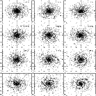
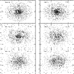
Spiral arm growth occurs with varying rates and amplitudes. Growth is not smooth or continuous. Frequently arms change shape, stretch, or break off and drift until hit by another passing disturbance. Well developed spiral arms, while subject to irregular change on short time scales, do survive. In figure 4, we show a series of snapshots of particle positions in simulation scv6, characterized by and an initial minimum . Instability first develops in the central regions of the disk, and propagates outward in radius. Even early () in the simulation, variations of density approach 10-50%; at late times they reach unity.
The dominant patterns are two and three-armed spirals with significant components having other symmetries. At late times we see multiple tails on a single arm, arms unevenly spaced in azimuth, and patterns which have one arm which is significantly stronger than its counterparts. Often such spacing and asymmetry is preceded by the breakup of an arm at its base, and subsequent drift through the disk or capture by another arm. For example, between the and the images, an structure breaks up, and reforms as an asymmetric spiral pattern. It then returns to its previous two armed structure by .
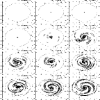
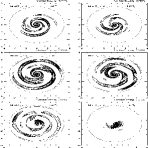
A comparable series of plots for a PPM simulation (pch6) with analogous initial conditions is shown in figure 5. The variable plotted is density variation defined by
| (12) |
where and refer to the grid indices of the and coordinates respectively, and is the azimuth average of the surface density at radial grid index . Only positive variation contours are shown. The linear spacing between one contour and the next higher contour is noted in the upper right hand corner of each plot. The dotted line denotes the disk edge at 50 AU. As in the SPH simulation, instability begins in the inner regions of the disk. Complex structures follow at midtime epochs. Later behavior shows well defined regular spiral patterns, with a mix of several patterns dominated by and which dynamically reorganize themselves with time.
The simulations above display a number of similar characteristics, though on a different spatial scale and mass distribution, to the protostellar core/inner disk simulations presented in Pickett et al. (1998). In each case, large scale spiral structures grow from marginally stable systems. The instabilities begin their growth in the innermost regions of the system and proceed to involve the entire disk as the simulation proceeds. At late times in both sets of simulations, the spiral arms become azimuthally condensed. A notable difference between our results and theirs, which will be discussed in section 4.3.2 below, is the fact that our simulations exhibit a pattern speed which increases toward the center of the disk. In contrast, Pickett et al. report constant pattern speeds.
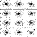
Initial behavior of our low disk mass runs is similar to those of high mass, with instabilities first becoming apparent in the inner regions of the disk. Evolution at later times differs from that for high mass disks. We see the rapid development of patterns with large numbers of spiral arms, which display a tenuous, filamentary structure not present in higher mass disks. The disk shown in figure 6 (simulation scv2) has a five armed pattern which predominates, and at late times fragments into multiple clumps from each arm. A region of apparent stability against spiral arm formation becomes apparent in the extreme innermost regions (see also section 4.2). Such regions are present to some extent in all of our SPH disks except those which form clumps immediately and are defined by a value of Toomre’s parameter greater than 2.
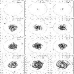
In a low disk mass PPM simulation (pch2), shown in figure 7, we also find a change in character and an increased number of spiral arms. As in figure 5, the instability begins to form its first spiral structures at amplitudes of 0.01-0.1%. Although the precise number of arms seen does not correspond to that in the SPH run (showing instead the 2-4 armed patterns dominant), the degree of small scale fragmentation in the region around 5-25 AU is similar. We believe that the partial suppression of the high -number patterns can be attributed to the wavelengths of those patterns approaching the gravitational softening length implied by the grid. This statement is supported by the fact that for the low mass disks (pch2 and pcm2), the amplitude of the perturbations , is larger in the higher resolution simulation. These simulations do not resolve the small scale structure. Note that the PPM run with () developed only minimal spiral structure after nearly six full disk orbit periods.
Structures observed in the moderate resolution PPM simulations (runs pcm1-pcm6) were qualitatively similar to those observed for our highest resolution runs (pch2, pch6), although the growth of the low mass/low resolution structures was slower. Growth rates are similar for the low and moderate resolution high mass disks. The simulations may have reached a level of convergence sufficient to resolve the large scale features of the evolution, but further improvement is desirable.
4.2 The Effects of Temperature
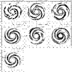
Two series of SPH simulations were run varying the minimum stability parameter , with mass ratios and . Other things being equal, high implies high temperature in the disk (eq. [6]). We vary for different simulations between a minimum value of , at which the disk is only marginally stable to ring formation, and a maximum value such that the outer edge of the disk remains bound. For the high mass series, this limit was found at , while for the lower mass disks up to were available.
In figure 8 we show ‘late time’ behavior of each of the disks in the series (sqh1-sqh6). Below an initial value of , strong instability and clump formation occurs during a few orbit periods of the inner portion of the disk. The outer disk remains largely unaffected during the simulation (which suffers drastic decreases in time step size once clumps form). At moderate (1.4 to somewhat less than 1.7), instability in the inner regions is slowed to the extent that spiral instabilities involving the entire disk have time to grow. These spiral arms then become filamentary and clump on time scales of one or two . The last few frames in figures 4 and 6 show such behavior for a disk with and and . The portions of the spiral arms at large distances from the central star remain thicker and more diffuse, while the inner regions evolve toward more sharply defined features. As increases the character of the spiral instabilities changes from narrow, filamentary structures and clumps in the inner disk to thicker arms which develop on disk orbital time scales at higher initial .
Above initial , we see only limited asymmetry and spiral structure. However, there is a strong transient epoch in which the centers of mass of the star and the disk orbit each other at large distances (relative to their late time behavior or to other, less stable (lower ) simulations). Simulations have been carried out to more than for these cases. This resonance gains in strength with increasing up to the maximum values simulated. Accretion of disk matter onto the star occurs at higher rates in these runs as well. The star makes a hole in which little disk matter remains.
Figure 9 shows an example of this transient for simulation sqh6. The orbit of the star begins with a slow transient to relatively large distances from the system center of mass (as large as in the disk shown). In the first , the star accretes a large fraction initially located in the inner part of the disk. After this time the star settles to a smaller orbit, with occasional fluctuations as it moves in response to disk perturbations, and continues to accrete from the inner disk. We believe this transient is largely due to the high mass accretion rates with nonaxisymmetric flow. With such fast accretion, the flow of mass onto the star is rapid enough that appreciable angular momentum is swept along as well. A comparable simulation, with the star fixed at the origin, shows nearly as large an accretion rate. We conclude that high accretion drives the stellar migration, rather than the reverse process where the star moves by some other means (caused for example by a torque from the outer disk) into a region of the disk in which high accretion may take place.
Although we find that the accretion rates seen in the most -stable disks are higher than low stability disks, it is not clear whether the magnitude of the accretion rates are correct. In SPH the accretion of a particle implies a sudden unphysical loss of pressure support to the neighbors of the accreted particle. As the disk reorganizes itself, additional particles move inward towards the accretion radius. If the mass accretion for all of our disks were to be scaled up or down by a common factor, the transient in figure 9 might increase or decrease in magnitude or even disappear. What we can say with certainty is that if a star can accrete matter from the inner disk quickly enough that it loses its pressure support further out, accretion of disk material which has not lost all of its orbital angular momentum can occur, driving the star away from the system center of mass. In the simulations we study here, such a condition occurs when the accretion rate is above /yr for the high mass series and /yr for the lower mass series.
Behavior of the lower disk mass series of SPH simulations with varied is similar. The overall characteristics of the evolution mimic that of the higher mass runs but are ‘stretched’ along the axis to higher values of . Azimuthal condensation of spiral arms is again seen up to initial , but the run at this mass ratio appears to be just beyond the critical stability for clumping: many preliminary characteristics of clumping such as well resolved spiral arms and short duration over-density spikes (see below) were evident but no actual formation occurred at the time we stopped the run at . Production of thick arms continues as high as and global star/disk resonances again manifest themselves all the way up to the maximum values studied. Distinct one-armed spiral waves form at for short periods, then lose coherency and fade back into a smooth, global pattern.
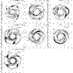
One series of PPM simulations was run with varying . The late time density variation contours for the series are shown in figure 10. Because of the low amplitude of the initial noise, these simulations were continued to even for the lowest minimum values. In the highest stability ( ) simulation, we find that the strength of the instabilities near the inner boundary dominate the instabilities over the disk as a whole. This instability does not seem to be the same as the transient seen in the SPH runs: it is limited to small radii inside the density maximum, and does not enter the outer disk at all. Because of the boundary behavior noted above, simulation of the disks into epochs having large amplitude variations was possible for only short times. We could not determine if a large transient in the orbits of the centers of mass of the star and the disk developed at late times for these simulations.
At low and moderate (), there is a great deal of correspondence between the qualitative results of our SPH and PPM runs. For simulations with moderate initial () multiple spiral arm structures develop with the and patterns most prominent. The pattern is present at varying levels as an asymmetric component of the dominant or 3 patterns.
For the lowest stability simulation, run at , density variations up to 40% are present in the disk and variations within a single spiral arm produce local density maxima within that arm. Continued collapse from large amplitude spiral structure into one or more clumps is not observed, probably because we have not resolved the gravitational potential or the rotational motion of the matter about a collapsing core to the necessary scale. The evolution of these lowest stability disks (i.e. simulation pqm1 and pqm2) at early times in the simulations are dominated by the growth of the pattern which, unlike their more stable cousins, is distinct even at the level. Later, these patterns tend to break up and reform as and patterns.
4.3 Spiral Pattern Growth
An important connection of numerical simulations to linear perturbation analyses is to define, if possible, the linearly growing spiral patterns of a system. To do so requires a specification of the growth rates and pattern speeds of the dominant spiral patterns in each system.
We compute the growth rates by first computing the amplitude of spiral patterns by Fourier transforming a set of annuli spanning the disk in the azimuthal coordinate. The amplitude of each Fourier component is then defined as , where is
| (13) |
for and the inner and outer radii of the disk are defined by and . The term is defined with a normalization of . With this normalization, the term is the mass of the disk and the amplitudes, , are dimensionless quantities. The phase angle is then defined from the real and imaginary components of the amplitude
| (14) |
Local amplitudes for each component can also be derived for annuli by neglecting the integration over radius in eq. [13]. Each Fourier component is computed about the center of mass of the system.
Assuming strictly linear growth for each Fourier component, we can use least squares techniques to fit a growth rate, , to each amplitude as a function of time with the equation
| (15) |
where is an constant defining the initial amplitude of the component. If we keep track of the number of times, , a pattern has wound past a phase angle of 2 and add to the derived phase at each time, we can derive a pattern speed by a similar fit as
| (16) |
This definition effectively averages over all short term variations (if any) in the pattern speed. A periodogram analysis gives similar results to this fit technique. The frequency with which we produce dumps of the simulation is sufficient to produce accurate pattern speeds over all but the inner AU of our disks, and over the full radial extent of the tori (see section 4.3.1).
We may independently derive an additional global growth rate for the component by noting that it is the only component which can contribute to the motion of the star. All higher order components are symmetric under a rotation smaller than 2 radians (i.e. respectively for each Fourier component) and therefore do not contribute to the motion of the disk center of mass. By fitting the distance between the centers of mass of the star and disk as a function of time, we find a growth rate independent of the precise geometry of the spiral arms in the disk. In general we find good agreement between this growth rate and the value derived from the above procedure.
The analysis of the pattern growth in disks and tori can proceed at either a local or a global level by either including or excluding the integration over radius in eq. [13]. If we derive a growth rate and pattern speed in a succession of narrow rings in the system and compare the values over the entire system, we can readily identify structures which are coherently growing and moving over large temporal and spatial scales. This feature is limited in a global analysis because the integration effectively averages the amplitude and speed of a given pattern over the entire system.
On the other hand, a local analysis can be quite misleading. If we consider a series of concentric narrow rings making up a disk, we must account not only for the growth of instability within any given ring, but also for the transport of already formed instabilities from one ring to another. For example: if some ‘lump’ of matter grows in one ring in the disk, then moves by some process to a second, the amplitude of the Fourier components in each of those rings will be affected: one will exhibit a net loss in amplitude, while the other a net gain. A growth rate based upon amplitudes affected by such processes would no longer represent the physical instability mechanisms present in the disk.
In the analysis that follows, we shall use a local analysis to identify patterns which are growing coherently over large spatial scales, but in order to compare our results to the global analyses of ARS and STAR, we shall utilize globally integrated quantities.
4.3.1 SPH and PPM: A Direct Comparison of Results and Numerics
Each code does well with different aspects of the evolution of disks. For the example of the disks discussed here, the low noise in the PPM calculations allows an accurate growth rate calculation, but with our treatment of boundaries, problems develop as a simulation becomes nonlinear. Matter reflected from the boundaries changes the total momentum of the system to such an extent that its center of mass (exhibited particularly in the position of the star) attempts to move to infinity. Because of its ability to dynamically adapt the available resolution to the interesting parts of the flow and relative sensitivity to boundaries, SPH is able to follow the nonlinear evolution much further. These same features however, forbid simulating a disk with a low density central hole because the steep density gradient near the inner disk edge cannot be adequately resolved at a computationally affordable level. Even for disks without a hole (for which the gravitational softening at the inner boundary blurs the physics and allows the simulation to proceed), the initial noise in SPH (of order ) leaves very little time for random perturbations to organize themselves into ordered global spiral structures while remaining in the linear regime.
Fitting growth rates to the SPH simulations requires much more caution than is required for the PPM runs. The initial noise level is such that only a very short time baseline is available prior to saturation. Typically, we observe a period during which Fourier components grow linearly until reaching a saturation level. This period of linear growth lasts for about one disk orbit or less for SPH and 2–3 for the PPM simulations.
The SPH disk simulations often reach high perturbation amplitudes close to the star before more distant regions of the disk have become active. To compare the two numerical methods and minimize this time scale problem, we have simulated relatively narrow tori. Such tori have a much more restricted dynamic range than a disk, so that the entire system becomes active at once. We use a torus with an outer to inner radius ratio of and a equation of state given by eq. [10] with temperature, density and individual particle mass given by a Gaussian function of radius
| (17) |
where is defined at the midpoint, , of the torus and , so that the torus extends about three ‘standard deviations’ in either direction from the highest density point (figure 11). Each simulation is then evolved isothermally in the same way as is done with our simulations of disks.
With a equation of state, it is difficult to find toroidal configurations which are initially stable to axisymmetric perturbations (i.e. everywhere), except for relatively low mass tori. For a variety of temperature or density laws, either the high density central region will collapse (i.e. the initial will be less than unity), or the outer edge will be unbound. For our test problem, a ratio of yields a minimum of about near the center of the torus. As before, the star mass is , the outer torus radius of =50 AU, and thus the outer edge of the torus orbit period is 500 yr.
Table 3 summarizes the characteristics of the simulations. The linear and nonlinear regimes are divided by the condition that the amplitudes of Fourier components other than the dominant pattern (or patterns) reach comparable amplitudes to that dominant pattern, and total perturbations reach 10%.
One SPH and two PPM simulations were run with this toroidal configuration at a resolution of cells for the PPM runs and particles in the SPH run. One PPM simulation with initial random noise amplitude (comparable to the initial noise in SPH) and one with noise of amplitude were run. The noise is input as a random density perturbation in each cell as
| (18) |
where and refer to the radial and azimuthal grid indices and is a pseudo-random number between zero and one. The amplitude noise is derived from truncation error in the initial state. Boundary conditions are identical to those used in our disk simulations.
The relatively large amplitude of the noise in the SPH simulations is caused by smoothing over a finite number of neighbors (see Herant and Woosley 1994). Increasing the number of neighbors used in the interpolation has a small effect in decreasing the noise amplitude but at a high computational cost. We have used a varying number of neighbors (depending on local conditions of the run) with a distribution centered near 15–20 neighbors per particle, a number which is standard for two dimensional simulations.
The resolution of features within the torus or disk must inevitably be less accurate in a finitely resolved system than in a physical system. PPM spreads shocks over at least two cells, for example, while further loss of resolution may come from the representation of the gravitational potential. In SPH, resolution is limited by the smoothing length of the particles and the artificial viscosity required to adequately reproduce shocks.
Two additional PPM and two additional SPH simulations of tori have been run to test resolution. One PPM run has 1.5 times the resolution in each dimension (60225–roughly doubling the number of cells) and the second twice the resolution (80300–quadrupling the number of cells). The SPH simulations increase by a factor of two and a factor of four the number of particles in each simulation. Comparing runs of different resolution is difficult, however, because the power spectrum of the initial perturbations may not be controlled to the limit required. In an attempt to duplicate the perturbation at low and high resolution, but remain above the uncontrollable level imposed by the grid itself, we have input an initial random noise amplitude of in each 22 block of cells in each of the two higher resolution PPM runs.
We show the evolved configuration of each run in figure 12. The time at which each is shown is near the linear regime cut off discussed below. The SPH runs are mapped onto a grid and plotted in the same manner as the PPM runs in order to make the visual comparison as direct as possible. In each of the runs, instability growth is dominated by spiral patterns with the higher resolution runs tending to show progressively less of the pattern and more of the pattern. The pattern predominates in each simulation except for the two low resolution PPM runs. The change in morphology in different simulations is probably an artifact of the resolution. As we show for the growth rates below, the lowest resolution simulations are apparently not converged.
In comparison, the results of Laughlin & Różyczka (1996) show a dominance of an component without a large presence of other patterns. The origin of instabilities in their systems is attributed to the family of vortensity instabilities with corotation exterior to the torus. Different initial conditions seem to be responsible for the rather than dominance. Our test simulations use a narrower torus than theirs, with an isothermal rather than adiabatic equation of state. A simulation with an identical initial condition and equation of state compares favorably to their results.
The amplitudes and fits for growth rates for the spiral pattern at the center of the torus (at AU) are shown for each simulation in figure 13. The fit parameters are derived from only the portion of the curve in which the patterns are growing and little disruption of the large scale structure of the tori has begun. This disruption is characterized by an onset of fragmentation at the inner and outer edges of the torus (SPH) or significant radial distortions in the torus (PPM). We also allow a short period () prior to the first fitted time point, for some initial transients (eg. the unphysical ‘ringed’ structure in the SPH initial state) to settle.
The pattern speeds and growth rates for the patterns are shown in figure 14 for each of the PPM simulations and in figure 15 for each of the SPH simulations. The pattern speeds for the patterns for each of the runs agree for both codes over the range of resolution and initial perturbation amplitude. The growth rates from the SPH simulations differ by as much as 50% between runs. For the SPH simulations obtaining a constant rate across each ring in the torus was not possible. For the PPM simulations, the growth rates near the inner and outer boundaries of the tori are reduced due to the fact that perturbations there do not begin to grow until after the denser regions of the torus have been disturbed. A similar effect is found for the pattern speed near the inner edge.
The growth rates for the SPH runs are affected by the high amplitude of perturbations in the initial state and the short time span over which the fit must be derived. Longer lived initial transients caused by the excitation of multiple eigenmodes of the system or by small inhomogeneities in the initial state can cause the amplitude curves to become quite nonlinear in form. The PPM simulations have longer time baselines so such transient effects are less important.
The growth rates for the pattern in the PPM simulations decrease with increasing resolution, while the and 3 growth rates are less affected. This fact and the trend towards and 3 spiral patterns for higher resolution runs suggest that they may be true linearly growing patterns for the system. The change in character with increasing resolution may be due to the fact that the torus begins its life very close to the stability limit, . Any inaccuracies in the resolution of the gravitational potential or the mass distribution (hence the pressure) will have their greatest effect in such a circumstance. The SPH simulations show no comparable effect, but reliable local growth rates can not be obtained for those simulations.
Late in each simulation the tori collapse into several condensed objects, but the details of the collapse vary. Not all of the spiral arms present during the growth of structure condense into separate objects. In many cases the spiral arms break up and/or merge as clumps begin to form. Figure 16 shows snapshots of each of the runs at the time at which the spiral arms begin to collapse. Each simulation is halted at this point because of the influence of the boundaries on the simulation and because we did not properly simulate the physics important in the collapsed objects. The structures which develop resemble the simulations discussed by Christodoulou & Narayan (1993) because the tori tend to deform radially as instabilities grow. With both codes the torus becomes so distorted radially that a line of condensations forms from the torus matter which has moved outwards.
We now summarize the similarities and differences between the results of each code.
Each code produces instabilities which grow in the tori as they evolve forward in time. The instabilities produced are multi-armed spirals structures which, at the end of each simulation, have begun to radially distort the torus and collapse into clumps. In both codes predominantly 2–4 armed spiral structures are produced. The high resolution simulations each produce 2 and 3 armed structures while low resolution simulations (apparently incompletely converged), produce predominantly 3 and 4 armed structures.
The initial state of an SPH simulation begins with random noise of amplitude above or below an ‘ideal’ initial value. Near the boundaries, where particles are not distributed evenly with respect to each other, additional differences from an ideal initial state are present. PPM can begin with noise in the initial state as small as machine precision for any given simulation.
The differences between one code and the other can be attributed to several effects. First, perturbations in the initial state may trigger more than one true eigenmode of the system which, taken together, cause more or less observed growth in a given simulation with respect to another. Because the noise input for each code arises from such different sources, the stimulated pattern growth may therefore initially have a much different character. This growth rate variation is exhibited predominantly by the amplitude of a given pattern ‘waving’ above and below its true linear growth curve and, in essence, constitutes an error estimate for a calculated growth rate. The PPM simulations, for which the growth rates are calculated over longer time baselines and with a smaller initial noise amplitude per Fourier component are not nearly as strongly affected by such effects. We estimate errors of 10-20% in the growth rates due to this effect in the PPM simulations and perhaps an additional 20-40% in the SPH runs because of their very short time baseline. Pattern speeds do not seem to be as strongly affected by these transient effects.
The adaptive nature of the resolution and high noise in SPH causes small scale filamentary structures to become active and develop more quickly than in our counterpart PPM simulations, which are limited to the resolution of the fixed grid. SPH will tend toward developing grainy and filamentary structures quickly, perhaps to a larger extent than is physically the case.
Because the grid boundaries are far away from the main concentration of mass in the torus, they have only a small effect until late in any given simulation. Such is not true for the disk simulations using the PPM code so those simulations cannot be carried out far into the nonlinear regime due to the growing influence of the boundaries at late times. The physics important for the global dynamical evolution of the disk ranges over a dynamic range larger than we are able to simulate. The state at which the PPM runs must be terminated (with 10-20% perturbations) are qualitatively quite similar to those of the SPH runs over most of their duration. It may be that for the disks we discuss below, the PPM runs are representative of the linear regime, while the SPH simulations are our only representation of the late time nonlinear behavior of the system.
4.3.2 Pattern Growth in Disks
With a clearer understanding of the numerical properties of our codes on a test problem, we return now to the study of disks. Due to the high initial noise of the SPH runs and large radial extent of the disks we study, saturation at small radii often occurs well before the entire disk has become involved in the instability. Because of this noise we do not believe growth rates calculated from these simulations are reliable for any Fourier component except the globally integrated pattern (for which we have the behavior of the centers of mass of star and disk), and we limit discussion of the growth rates in this and the following sections to the PPM simulations.
The qualitative observations of sections 4.1 and 4.2 have shown that there is rarely a single spiral pattern present in a disk. More quantitative measurements show that growth is present in all Fourier components up to very high order. Such growth does not necessarily imply that actual spiral arms of that order are present in the simulation, but rather that the arms that do exist become more filamentary than pure sinusoids, creating power in higher order Fourier components (a Dirac -function will yield power at all wave numbers for example). In order to be more definitive regarding the true morphology of each disk we visually examine each simulation and tabulate the dominant spiral patterns in Tables 1 and 2.
Which patterns represent linear growth in each of the systems? To begin to answer this question we must fit growth rates and pattern speeds to the various spiral patterns present in each disk and determine which patterns exhibit rates which are constant at differing resolution, across a large portion of the system and over a large time period. In figure 17 we show the amplitude of the and patterns as a function of time near the middle of the power law portion of the disk and integrated over all radii for our prototype massive disk shown in figure 5. Over long periods the growth is essentially linear in character. Over shorter periods it is punctuated by transients which can change the amplitude by up to an order of magnitude. The amplitude variations apparently arise as short-lived structures successively grow and fragment throughout the disk. Time dependence of pattern speeds within the disk will be discussed in section 4.3.4 below.
Radius dependent growth rates and pattern speeds for the are shown in figure 18 for two different grid resolutions. The growth rates and pattern speeds are similar at both resolutions, suggesting that the simulations may have resolved the physical processes important in this disk. The growth rates for the patterns are nearly constant with radius but the pattern speeds derived are not at all constant with radius; they decrease as a steep function of the distance from the central star.
Low mass disks show a marked absence of the dominant low order () spiral patterns so common among higher mass disks. Typically, the amplitudes and growth rates of all Fourier components are comparable. We plot the growth rates and pattern speeds for the same patterns () as above for our prototype low mass disk in figure 19. We again find that the pattern speeds are steeply decreasing functions of the radius. We also find that the growth rates do not exhibit the same values for different grid resolutions. This fact suggests that the low mass disks have not fully converged at the grid resolution used in our simulations. The systematic trend towards faster growth in the higher resolution simulation indicates that the small scale features which dominate the morphology of this system may be somewhat inhibited by the resolution of the gravitational potential and the hydrodynamic quantities on the grid. Much higher resolution simulations are required to be able to fully resolve the features important for disks of mass less than than are required for more massive systems.
With simulations of varying stability we would ordinarily expect larger values to lead to slower instability growth. Similarly, we expect smaller values should imply more rapid growth of instability. In fact, as discussed in section 4.2, both extremes lead to rapid instability growth, but of different character.
Although it begins with an extreme initial condition, the simulation pmq5 (with , ) shows an interesting example of the limiting behavior displayed in a highly stable disk ( everywhere) with a turnover in its density profile near the central star. We show the and pattern amplitudes at two locations in the disk and integrated globally in figure 20. In this simulation, rather than being suppressed, the amplitude of the instabilities begins to grow quickly in a region limited to the innermost portion of the disk. Further out in the disk much slower growth occurs. The development of such instabilities in disk systems cannot be attributed to a global, linearly growing phenomenon; its localized character and the different behaviors of the amplitude growth at different locations in the system argue against that. It remains unclear to what extent this type of growth happens in real systems, but it seems that with a turn-over in the density law at small radii or the less severe case where the density law flattens (as in our SPH simulations) can lead to increased local instabilities.
It is interesting to note that Pickett et al. (1996) report similar behavior (which they refer to as ‘surge’ growth) in several of their more -stable simulations. In their work however, the initial mass distribution and and rotation curve are somewhat different than in our own work. The fact that similar behavior is observed in simulations of such different character suggests a similar mechanism may be driving the evolution of both sets of simulations.
The lowest stability simulations also show rapid growth of spiral instabilities. In these simulations there are no growth features similar to the ‘hump,’ or sudden rise in amplitude shown in figure 20. In general, the qualitative features of the growth are similar to those seen in figures 17 and 18 but with as much as 50–100% larger growth rates in the case of the lowest stability run (pmq1).
The results of our analysis in this section show that in spite of its large amplitude at early times and its continued presence for the duration of the run, our simulations do not show evidence of a pure pattern. In no case is the growth rate or pattern speed constant across a large portion of the disk. In contrast to several higher patterns, the wide variation is true of both the growth rate as well as the pattern speed. Because of the variation of the growth rate and pattern speed we must conclude that a direct connection to the SLING mechanism is not possible. At the high amplitude (late time) phase of evolution shown in the SPH simulations, the and patterns have become dominant for disks more massive than , while at the lower amplitudes typical of our PPM runs, has the largest amplitude, though the pattern itself is ordinarily seen only as asymmetries in higher structures.
None of the disk simulations we have performed produce pattern speeds for any pattern which are constant across the entire disk. The growth rates, while ordinarily stable at a single value over the whole system for at least some patterns (see eg. fig. 18), do not reflect the short term behavior of the system as structures fragment or deform over time. In this case the ‘linear growth modes’ of the system, defined as the complex eigenvalue of a system of equations, become difficult to define or to interpret.
4.3.3 Suggestions for the Mechanisms of Instability Growth
In each of our simulations, instabilities are generated in the innermost portions of the disk, eventually impacting the entire system. Such growth occurs in spite of the fact that the inner regions are the most stable as measured by two of the classic stability indicators, namely the Toomre criterion and the SWING parameter. If we are to suggest a mechanism for the instability growth we are limited to mechanisms which can produce instabilities in what are ostensibly highly stable regions.
We have already discussed the possibility that in some cases instabilities may due to nonaxisymmetric accretion of disk matter onto the star or by accretion of infalling material onto the disk, rather than to dynamical instabilities in the disk itself. In other cases, the vortensity based instabilities of Papaloizou & Lin 1989 (see also Adams & Lin 1993) may provide an answer because they can grow in highly ‘stable’ regions and their growth can be local in nature. They discuss three classes of vortensity instabilities which can exist in a disk: those dependent on vortensity extrema within the disk or at its edge (‘edge modes’), those dependent on resonances (‘resonance modes’), and those which have corotation exterior to the disk (dubbed ‘slow modes’ and studied extensively by Laughlin & Różyczka 1996). Because we find corotation within the disk for most times (though at varying position), we can eliminate the last of these classes from consideration. The remaining two, we believe, are both active at different times and to a greater or lesser extent in the disks we model. At early times, our initial condition (the softened power law or density turn-over at small radii) implies a vortensity extremum near the inner boundary of the disk. This condition may excite an edge mode which over time propagates outward over the density maximum in our PPM simulations via a resonance mode into the disk, exciting global instability channels such as SLING as it propagates into the main disk. We have not established a definite connection between the instabilities in our simulations and the vortensity based instabilities however.
We cannot definitely connect the SLING instability directly to phenomena present in our simulations; see section 4.3.2. We may still perhaps be able to make qualitative connections between phenomena predicted to be important via linear analyses and our results. One example of such phenomena would be growth rates which depend upon the outer boundary condition imposed. Another might be a growth rate which, as a function of disk mass, increases for disks more massive than some critical value, as suggested by the ‘maximum solar nebular mass’ discussed in STAR. Such characteristics would not necessarily be limited to the pattern but may also exist in patterns as well.
We do see such characteristics in the variation of the growth rates with respect to the disk/star mass ratio. For each series of PPM simulations varying disk mass, figure 21 shows the value of the globally integrated growth rates for the patterns. Growth rates for other patterns appear qualitatively similar to those shown. As one expects, growth rates of the highest mass disks are the largest, while instabilities in low mass disks grow much more slowly. In the reflecting boundary runs, a distinct ‘turn on’ mass is evident between , a value which corresponds to the ‘maximum mass solar nebula’ predicted by the results of STAR. The infall series does not exhibit such a distinct onset, but rather a continuous rise to a plateau which does not flatten out until the mass ratio reaches .
For low disk masses, the growth rates for each pattern are of order . These rates are comparable to the rate attributable to numerical effects. The numerical effects have their origin primarily in the fact that mass interacting with the grid boundaries gives an impulse to the system center of mass, which must be stable in order to determine the amplitude of the spiral pattern. Higher patterns are also affected as spiral waves reflect off the grid boundaries back into the simulation.
For higher mass disks, the outer boundary has a marked influence. As ARS predict, details of the outer radial boundary are an important factor in the growth pattern. The simulations with matter infalling onto the outer disk edge develop spiral structure with growth rates as much as 2-3 times faster than with a purely reflecting boundary. Simulations at two resolutions were run with an infall boundary to test the degree to which numerical effects of the boundary were affecting the growth. Both series show similar growth rates (fig. 21).
4.3.4 Importance of Phenomena not Included in Linear Analyses
On short time scales the pattern speeds in our disks can vary by as much as 100%. One example, shown in figure 22, is taken from the high mass disk simulation pch6. There we show the instantaneous pattern speed for the pattern near the middle of the disk, as calculated by numerically differencing the pattern phase , at successive output dumps of the simulation. Such variations in time are typical of each pattern in each disk simulation we have performed, and appear in both local and globally integrated pattern speeds. Pattern speeds calculated this way for the torus simulations of section 4.3.1 show much slower variations.
In the case of the pattern, whose global pattern speed is reflected in the motion of the star, we find that the star occasionally loops back upon its own trajectory and counter-rotates with the disk for a short period. Such a condition is not an uncommon occurrence in systems with disturbances with different orbital (pattern) periods. In our own solar system, for example, the sun’s motion about the solar system barycenter was retrograde most recently in 1990, when Jupiter was on the opposite side of the sun from the other three major planets.
The variations seem to arise because of the growth, fragmentation and reformation processes undergone by the spiral arm structures over the course of their evolution. Because the pattern speeds vary, an averaged pattern speed at any location in the disk (via eq. [16]) loses meaning and the location of the corotation and Lindblad resonances for each pattern also vary in time. When such variations are occurring, wave analyses, which typically assume stable resonances, may be of limited utility (wave analysis is of course useful in less chaotic circumstances–see, eg., STAR and Laughlin, Korchagin, & Adams 1996).
The growth of instabilities does not diminish as increases, but the instabilities do change character; this change is due to the increasing importance of effects not modeled in semi-analytic treatments of disks. For the high SPH runs, these effects are dominated by the nonaxisymmetric accretion of disk matter onto the star. As the star begins to move from the center of mass of the system (due to ordinary disk processes or the potential hump at the origin), some portion of the accretion becomes nonaxisymmetric. In the warmest disks, as much as 10% or more of the disk is accreted over the life of the simulation. Disk matter accreting onto the star sweeps along some residual angular momentum which is transferred to the star either as spin (an effect we neglect here) or as net angular momentum of the star about the system center of mass. In these cases, the star may gain enough momentum to be driven further away from the center of mass and create power in the pattern.
In the PPM runs with infall, the instability growth can include a component due to the outer disk edge perturbations. These may be due to infall itself, or to the fragmentation of the boundary. Although the linear analyses of ARS and STAR showed that the conditions at the outer boundary were important for the evolution of the system, they were unable to fully model the effects that the boundary can have on the system (see however Ostriker, Shu, & Adams 1992).
4.4 Clump Formation and Characteristics
Returning now to our SPH simulations, in this section we describe several qualitative features of clump formation and evolution in the disks. Due to the unsteady nature of the spiral instability growth and the presence of multiple spiral patterns in the system, each disk sequentially approaches and moves away from conditions in which clump formation is likely. These conditions are most readily apparent in plots of the minimum value in the disk and in the maximum over-density in the disk (defined as ) with respect to time.
The value of is defined rigorously only for an azimuthally symmetric disk. Nevertheless, as an indicator of the most unstable locations in the disk, we examine its value in nonaxisymmetric systems. To calculate its value locally we must first determine the epicyclic frequency at each point in the disk. We use the same procedure by which SPH obtains derivatives of all other hydrodynamic quantities. By definition
| (19) |
so the value , taken pairwise over each neighbor, is weighted using the SPH kernel. The result is summed to form a local value of the epicyclic frequency.
Plots of maximum over-density and minimum are shown in figure 23 for our two prototype SPH disks. Each variable is a global extremum. As such, the value of one could be determined from a completely different portion of the disk than the other. However, after only a relatively small fraction of an orbit time , the locations of minimum and maximum over-density are close, at a position between about 10 and 30 AU.
After a few orbit periods of the inner disk regions, the over-density rises to about twice its initial value (of unity). A slow secular trend towards stronger spiral arms over the course of the run follows, punctuated by one or more sharp, short-duration episodes of very strong activity in which density locally increases to 5-10 times. Over-density spikes become more and more frequent as the simulations progress, finally leading to clump formation. With the one exception , which, as noted in section 4.2, appears to lie on the ‘boundary’ between clumping and non-clumping disks, simulations which do not eventually form clumps also do not show these large over-density events. We attribute the origin of the over-density events in our simulations to the growth of spiral instabilities into a high amplitude nonlinear regime. In this regime spiral patterns present constructively interfere with each other or collide with other arms and orphaned arm fragments.
The results of Adams & Watkins (1995; hereafter AW) show that a density enhancement within a disk will lead to collapse if the condition
| (20) |
is met, where is the local value (azimuth average) of the Toomre parameter at the location of the density enhancement. For the disks in our study, this expression implies that an over-density factor of 3 or higher must be present in the disk, depending on where in a disk the collapse event occurs. This prediction is supported by our numerical results, which show that disks can survive (i.e. not exhibit collapse) for long periods with over-densities of 2-4, but collapse when over-density spikes of magnitude 6-10 occur.
For all disk masses, the minimum value of rapidly falls below its initial value to well below unity. After the initial steep decline, a slower decrease occurs until clumping begins and minimum falls to zero. The initial decline occurs most quickly in the highest mass disks, in which instabilities of any type are most strongly felt. With below unity, the disk becomes unstable not only to spiral instabilities but also to ring formation or, in the case of isolated patches, collapse. The collapse is slowed by the effects of rotation within the forming clump.
We can verify that it is rotation which slows the collapse by noting that the effects of the over-density spikes manifest themselves at only the 20-30% level in . We also know that the sound speed is constant in the proto-clump (due to our assumption that the disk evolves isothermally), from the definition of we know that the rotation of an individual proto-clump (really the shear across the clump, measured by the local value of the epicyclic frequency ) is the mechanism which inhibits further collapse. Only after spiral arm amplitude has reached sufficient levels to overcome rotation can an irreversible collapse begin.
Clumps condense out of the spiral arms on quite short time scales in even the least massive disks. During and after the initial stages of their formation, we find that the clumps show prograde rotation. No clumps were seen to form in any disk studied whose initial was greater than 1.5. Clump formation is most common at radii less than and usually several clumps will form from the same disk (and even within the same spiral arm). Less massive disks form many low mass clumps and higher mass disks form 2-4 higher mass clumps. The mass inside the clumps is of order 1% of the star mass at the time each simulation is ended. It is clear, however, that from the amount of remaining disk that no final mass has been determined.
The clumps form with such vigor in each of these disks because of the strong cooling implied by the isothermal assumption. Any density enhancements like those seen in figure 23 instantly lose their pressure support and collapse rather than dispersing. With more realistic cooling, the clumping behavior seen in our results may change. Thus our results are most useful as an indication of the behavior of disk clumping and as indicator of where clumps may be most likely to form in more physically realistic disks.
Figure 24 shows a plot of the radius at which each clump formed for each disk in the series. Only in the case of the disk, in which clump formation is prolific in nearly all regions, were any clumps formed at radii greater than 0.5 . With this exception, we believe the variation in the locations of clump formation in disks of different mass in figure 24 to be due more to stochastic effects rather than any physical process. To test this idea we ran a comparison series of simulations (’s), utilizing the Lagrangian version of the equation of state. When such an assumption is made, the background noise inherent in the code changes character. No overall structural changes are evident in figure 24, but differences in detail are present. Also, for the disk with , clumps were not formed at the largest radii. We believe this lack of clumps is due in part to the radial motion of some warmer particles into the outer disk, causing clumping to be suppressed.
The prior results of AB92, in which clumps are seen to form at much larger radii, correspond to a somewhat different initial configuration. In particular, our present results use a much smaller ‘core radius’, , for the density and temperature power laws. The gravitational softening parameter for the star is correspondingly smaller, and no initial perturbations are assumed. These differences conspire to push collapse instabilities to larger radii in the AB92 results, since in their simulations more mass is concentrated at large distances from the star. We believe the present conditions to be more realistic and thus to represent an improvement over the AB92 results.
4.4.1 Initial Orbital Characteristics
Out of the entire sample of newly formed clumps, none have an initial eccentricity much higher than , and most are between zero and 0.1. The low mass companions now being discovered around nearby solar type stars show both small and large values of eccentricity (Mayor et al. 1997; Marcy & Butler 1995; Butler & Marcy 1996). Although the clumps in our simulations form only in relatively low eccentricity orbits and are therefore dissimilar to many of those being discovered, considerable evolution of eccentricity can take place between the times corresponding to the end of our simulations and the final morphology of the system (see e.g., Artymowicz 1993, 1994; Goldreich & Tremaine 1980).
5 Conclusions
By using two conceptually different hydrodynamic methods (SPH and PPM), we are able to simulate a broader range of problems, but gain a sobering insight into the limitations of these tools. It is striking that PPM indicates violent behavior near the inner boundary (weakly supported by SPH), and that SPH indicates pronounced clumping (weakly supported by PPM). Both methods indicate that instability growth is not a steady progression from low to high amplitude perturbations with a single dominant pattern present throughout. Both methods indicate a marked change in the character of instabilities with disk mass. Low mass disks form many armed filimentary spiral structures while high mass disks form few armed grand design spiral structures.
In this study of the evolution of circumstellar accretion disks, we have found simultaneous growth of global spiral instabilities with multiple Fourier components. Growth of each of the components occurs over the course of a few orbit periods of the disk and a single component rarely dominates the evolution of a disk. As expected, the massive disks are found to be the most unstable, due to self-gravitating instabilities within the disk. Accretion of matter onto the star itself can, in warm disks (i.e. those with high values), significantly drain matter from the disk on similar time scales to the self-gravitating instabilities. Short-term variations in the amplitude of a given component, and strong constructive interference behavior between different components, can produce ‘spikes’ in the surface density. These spikes can eventually grow to such amplitude that gravitational collapse occurs resulting in the production of one or more clumps.
Pattern growth is stimulated at early times by the rapid growth of instabilities at small radii which eventually engulf the entire disk. Steady spiral arm structures are not generally present. Instead, spiral arms progressively grow, fragment and reform as time progresses. In cases where accretion is rapid, power can be produced in an spiral pattern due to nonaxisymmetric accretion of mass and momentum onto the star. Understanding the dynamics of the inner region is of primary importance for understanding the global morphology of the system.
The gross structure of low and high mass disks are markedly different from each other. High mass disks form large, grand design spiral arms with few arms, while low mass disks form predominantly thin, filamentary multi-armed structures. In almost no case is the spiral pattern the fastest growing pattern in the disk. Typically a combination of patterns in high mass disks or very high order patterns () in low mass disks dominate the morphology. The transition between these behaviors comes at approximately . This transition corresponds to the ‘maximum solar nebula’ mass discussed in STAR, above which modes due to SLING are expected to grow strongly.
It is intriguing to speculate that the collapse processes seen here are responsible for the production of brown dwarf-like companions such as that seen by Nakajima et al. (1995) and/or of planetary companions similar to those recently discovered around several nearby stars (Mayor & Queloz 1995, Marcy & Butler 1996, Gatewood 1996). However, we must emphasize that clump formation in self-gravitating circumstellar disks depends on the ability of the gas to cool efficiently. Our simulations here use a simple isothermal equation of state which favors clump formation. Additional simulations with realistic cooling functions, including radiative transfer effects, must be done in order to clarify this important issue.
References
- (1)
- (2) Adams, F.C. & Benz, W., 1992, Gravitational Instabilities in Circumstellar Disks and the Formation of Binary Companions, in Complementary Approaches to Double and Multiple Star Research, IAU Colloquium No. 135, (Provo: Publications of the Astr. Soc. of the Pac.) (AB92)
- (3)
- (4) Adams, F. C., Emerson, J. P. & Fuller, G. A. 1990, ApJ, 357, 606
- (5)
- (6) Adams, F. C. & Lin, D. N. C., in Protostars and Planets III, ed. Lunine, J. I. and Levy, E. H., Tucson: University of Arizona Press
- (7)
- (8) Adams, F. C., Ruden, S. P. & Shu, F. H., 1989, ApJ, 347, 959 (ARS)
- (9)
- (10) Adams, F. C. & Watkins, R., 1995, ApJ, 451, 314
- (11)
- (12) Artymowicz, P., 1994, ApJ, 423, 581
- (13)
- (14) Artymowicz, P., 1993, ApJ, 419, 166
- (15)
- (16) Artymowicz, P., & Lubow, S., 1994, ApJ, 421, 651
- (17)
- (18) Balsara, D., 1995, J. Comp. Phys, 121, 357
- (19)
- (20) Bate, M., Bonnell, I. & Price, N. M., 1996, MNRAS, 277, 362
- (21)
- (22) Beckwith S. V. W., Sargent, A. I., Chini, R. S. & Güsten, R. 1990 AJ, 99, 924
- (23)
- (24) Benz, W., 1990, in The Numerical Modeling of Nonlinear Stellar Pulsations p. 269, J. R. Buchler ed.
- (25)
- (26) Benz, W., Bowers, R. L., Cameron, A. G. W. & Press, W. H. 1990, ApJ, 348, 647
- (27)
- (28) Binney, J., & Tremaine, S., 1987, Galactic Dynamics, Princeton: Princeton University Press
- (29)
- (30) Boss, A., 1995, ApJ, 439, 224
- (31)
- (32) Bonnell, I. & Bastien, P., 1992, ApJ, 401, 654
- (33)
- (34) Burkert, A. & Bodenheimer, P., 1993, MNRAS, 264, 798
- (35)
- (36) Cassen, P. M. & Moosman A., 1981. Icarus, 48, 353
- (37)
- (38) Christodoulou, D. & Narayan, R., 1992, ApJ, 388, 451
- (39)
- (40) Colella P. & Woodward, P. R., 1984, J. Comp. Phys., 54, 174
- (41)
- (42) Duquennoy, A., & Mayor, M., A&A, 248, 485
- (43)
- (44) Foster, P. N. & Boss, A. P., 1996, ApJ, 468, 784
- (45)
- (46) Fryxell, B. A., Müller, E. & Arnett W. D., 1989, Max Plank Institut für Astrophysik Report #449
- (47)
- (48) Fryxell, B. A., Müller, E. & Arnett W. D., 1991, ApJ, 367, 619
- (49)
- (50) Gatewood, G., 1996, BAAS, 28, 885
- (51)
- (52) Ghez, A., Neugebauer, G., & Mathews K., 1993, AJ, 106, 2005
- (53)
- (54) Goldreich, P., & Tremaine, S., 1980, ApJ, 241, 425
- (55)
- (56) Heemskirk, M. H. M., Papaloizou, J. C. B. & Savonjie, G. J., 1992 A&A, 260, 161
- (57)
- (58) Herant, M., & Woosley, S. E., 1994, ApJ, 425, 814
- (59)
- (60) Laughlin, G. & Bodenheimer, P., 1994 ApJ, 436, 335
- (61)
- (62) Laughlin, G., Korchagin, V. & Adams, F. C. 1996, ApJ, 477, 410
- (63)
- (64) Laughlin, G., & Różyczka, M., 1996 ApJ, 456, 279
- (65)
- (66) Leinert, Ch., Zinnecker, H., Weitzel, N., Christou, J., Ridgway, S. T., Jameson, R., Haas, M. & Lenzen, R., 1993, A&A, 278, 129
- (67)
- (68) Lynden-Bell D. & Pringle, J. E., 1974, MNRAS, 168, 603 (LBP)
- (69)
- (70) Marcy, G. W., & Butler, R. P., 1996, ApJ, 464, 147
- (71)
- (72) Mayor, M., & Queloz, D., 1995, Nature, 378, 355
- (73)
- (74) Mayor, M., Queloz, D., Udry, S., Halbwachs, J.-L., 1997, From Brown Dwarfs to Planets, in Astronomical and Biochemical Origins and Search for Life in the Universe, IAU Colloquium No. 161, (Bologna, Italy: Editrice Compositori).
- (75)
- (76) Monaghan, J. J., 1992, ARA&A, 30, 543
- (77)
- (78) Murray, J., 1994, PhD thesis: Monash University
- (79)
- (80) Myhill, E. A. & Kaula, W. M., 1992, ApJ, 386, 177
- (81)
- (82) Nakajima, T., Oppenheimer, B. R., Kulkarni, S. R., Golimowski, D. A., Matthews, K. & Durrance, S. T., 1995, Nature, 378, 463
- (83)
- (84) Ostriker, E. C., Shu, F. H., Adams, F. C., 1992, ApJ399, 192
- (85)
- (86) Papaloizou, J. C. B. & Lin, D. N. C., 1989 ApJ, 344, 645
- (87)
- (88) Papaloizou, J. C. B. & Savonjie, G. J., 1991, MNRAS, 248, 353
- (89)
- (90) Pickett, B. K., Durisen, R. H., & Davis, G. A., 1996, ApJ, 458, 714
- (91)
- (92) Pickett, B. K., Cassen, P., Durisen, R. H., Link, R., 1998, ApJ, preprint
- (93)
- (94) Porter, D. H. & Woodward, P. R., ApJS, 93, 309
- (95)
- (96) Shakura, N. J. & Sunyaev, R. A., 1973, A&A, 24, 337
- (97)
- (98) Shu, F. H., Adams, F. C. & Lizano, S., 1987 ARA&A, 25, 23
- (99)
- (100) Shu, F. H., Tremaine, S. Adams, F. C. & Ruden, S. P., 1990 ApJ, 358, 495 (STAR)
- (101)
- (102) Simon, M., Ghez, A. M., Leinert, Ch., Cassar, L., Chen, W. P., Howell, R. R., Jameson, R. F., Matthews, K., Neugebauer, G. & Richichi, A., ApJ, 443, 625
- (103)
- (104) Terebey, S., Shu, F. H. & Cassen, P., 1984 ApJ, 286, 529.
- (105)
- (106) Woodward, J. W., Tohline, J. E. & Hachisu, I., 1994, ApJ, 420, 247
- (107)
| Name | Number of | End Time | DominantaaWhen only m=1 patterns are indicated, actual evolution is apparently an accretion induced transient star/disk oscillation (see figure 9) rather than a spiral arm. NR (not resolved): for low stability disks, assignment of specific spiral arm patterns loses meaning due to their rapid breakup. | Number | ||
|---|---|---|---|---|---|---|
| Particles | (=1) | Spiral Pattern | of Clumps | |||
| scv0 | 7997 | .05 | 1.5 | 3.5 | 6 | |
| scv1 | 7997 | .1 | 1.5 | 1.6 | 10 | 14 |
| scv2 | 7997 | .2 | 1.5 | 1.6 | 5-6 | 33 |
| scv3 | 7997 | .4 | 1.5 | 1.7 | 3-4 | 7 |
| scv4 | 7997 | .6 | 1.5 | 1.7 | 2-4 | 6 |
| scv5 | 7997 | .8 | 1.5 | 2.4 | 1-3 | 3 |
| scv6 | 7997 | 1. | 1.5 | 1.8 | 1-3 | 3 |
| sqh1 | 7997 | .8 | 1.1 | 0.1 | NR | 18 |
| sqh2 | 7997 | .8 | 1.3 | .25 | NR | 11 |
| sqh3 | 7997 | .8 | 1.4 | .35 | NR | 7 |
| sqh4 | 7997 | .8 | 1.7 | 4.2 | 1-2 | 0 |
| sqh5 | 7997 | .8 | 2.0 | 4.2 | 1 | 0 |
| sqh6 | 7997 | .8 | 2.3 | 4.2 | 1 | 0 |
| sql1 | 7997 | .4 | 1.1 | .15 | NR | 28 |
| sql2 | 7997 | .4 | 1.3 | 0.3 | NR | 7 |
| sql3 | 7997 | .4 | 1.4 | 0.4 | 4 | 1 |
| sql4 | 7997 | .4 | 1.7 | 5.0 | 1-3 | 0 |
| sql5 | 7997 | .4 | 2.0 | 4.2 | 1-2 | 0 |
| sql6 | 7997 | .4 | 2.3 | 4.2 | 1 | 0 |
| sql7 | 7997 | .4 | 2.7 | 4.2 | 1 | 0 |
| sql8 | 7997 | .4 | 3.0 | 4.2 | 1 | 0 |
Note. — Three series of runs are represented in this table. The first letter in each name is ‘s’, signifying an SPH simulation. The second, is either ‘c’ or ‘q’, signifying constant or varying , and the third letter signifies that the simulation is a member of a high (h), low (l) or varying (v) disk mass series. Ascending numerical order in each series refers to successive values of either disk mass or , for each series.
| Name | Grid | End Time | DominantaaNR: not resolved. For some low mass disks, distinct spiral patterns are not possible to distinguish. | Outer | ||
|---|---|---|---|---|---|---|
| Res. | (=1) | Spiral Patterns | Boundary | |||
| pcm1 | 64102 | 0.1 | 1.5 | 5.8 | NR | Refl. |
| pcm2 | 64102 | 0.2 | 1.5 | 5.0 | 2-4 | Refl. |
| pcm3 | 64102 | 0.4 | 1.5 | 4.0 | 1-3 | Refl. |
| pcm4 | 64102 | 0.6 | 1.5 | 3.75 | 1-3 | Refl. |
| pcm5 | 64102 | 0.8 | 1.5 | 3.0 | 1-3 | Refl. |
| pcm6 | 64102 | 1.0 | 1.5 | 3.0 | 1-3 | Refl. |
| pch2 | 100152 | 0.2 | 1.5 | 5.0 | 2-4 | Refl. |
| pch6 | 100152 | 1.0 | 1.5 | 3.6 | 1-3 | Refl. |
| pqm1 | 64102 | 0.8 | 1.1 | 1.8 | 1-2 | Refl. |
| pqm2 | 64102 | 0.8 | 1.3 | 2.6 | 1-2 | Refl. |
| pqm3 | 64102 | 0.8 | 1.4 | 3.0 | 1-2 | Refl. |
| pqm4 | 64102 | 0.8 | 1.7 | 3.0 | 1-2 | Refl. |
| pqm5 | 64102 | 0.8 | 2.0 | 2.0 | 1 | Refl. |
| pci2 | 6496 | 0.2 | 1.5 | 3.8 | 3-4 | Infall |
| pci3 | 6496 | 0.5 | 1.5 | 2.1 | 1-3 | Infall |
| pci4 | 6496 | 0.6 | 1.5 | 2.0 | 1,3 | Infall |
| pci6 | 6496 | 1.0 | 1.5 | 1.6 | 1-3 | Infall |
| pcl1 | 4464 | 0.1 | 1.5 | 5.6 | NR | Infall |
| pcl2 | 4464 | 0.3 | 1.5 | 4.2 | 1-3 | Infall |
| pcl3 | 4464 | 0.4 | 1.5 | 4.2 | 1-3 | Infall |
| pcl4 | 4464 | 0.5 | 1.5 | 2.8 | 1-2 | Infall |
| pcl5 | 4464 | 0.7 | 1.5 | 2.8 | 1-2 | Infall |
| pcl6 | 4464 | 1.0 | 1.5 | 2.0 | 1-2 | Infall |
Note. — Each of these PPM runs begins with ‘p’ to distinguish it from SPH series. The second letter is ‘c’ or ‘q’ signifying a constant or varying value for each disk in the series. The third letter implies a low, moderate or high resolution simulation. Moderate resolution infall boundary simulations are distinquished from reflecting boundary simulations using an ‘i’ in place of ‘m’. Numbers are successive values of disk mass or in each series of runs.
| Initial | Hydro | Linear | Reason/ | Non-linear | Reason/ |
|---|---|---|---|---|---|
| Density | Method | Regime | Result | Regime | Result |
| Structure | |||||
| Disk | PPM | fails | inner | inaccessible | |
| (eq. 3) | boundary | ||||
| SPH | inaccessible | short time | succeeds | spiral arm | |
| baseline | formation/collapse | ||||
| Disk w/ Central | PPM | succeeds | spiral arm | short | boundary |
| Hole (eq. 4) | growth | duration only | influence | ||
| SPH | inaccessible | short time | |||
| baseline | |||||
| Torus | PPM | succeeds | spiral arm | succeeds | spiral arm |
| (eq. 17) | growth | collapse | |||
| SPH | partial | spiral arm | succeeds | spiral arm | |
| success | growth | collapse |