Astrometric Observation of MACHO Gravitational Microlensing

Abstract

Following previous suggestions of other researchers, this paper discusses the prospects for astrometric observation of MACHO gravitational microlensing events. We derive the expected astrometric observables for a simple microlensing event with either a dark or self-luminous lens, and demonstrate that accurate astrometry can determine the lens mass, distance, and proper motion in a very general fashion. In particular we argue that in limited circumstances ground-based, narrow-angle differential astrometric techniques are sufficient to measure the lens mass directly, and other lens properties (distance, transverse motion) by applying an independent model for the source distance and motion. We investigate the sensitivity of differential astrometry in determining lens parameters by Monte Carlo methods, and derive a quasi-empirical relationship between astrometric accuracy and mass uncertainty.

1 Introduction

In 1986 Paczyński (Paczyński 1986b ) suggested that photometric observations of gravitational microlensing might be used to indirectly study the population of massive compact objects in the galaxy, and in particular MAssive Compact Halo Objects (MACHOs) that might be a significant component of the dark matter thought to exist in the galaxy by dynamical considerations. Paczyński’s 1986 paper, and the observational proposals it fostered were met with some skepticism. However, the past several years have seen Paczyński’s suggestion spectacularly confirmed – at the time of this writing four separate groups have reported significant numbers of candidate gravitational microlensing events from photometric observations of LMC, SMC, and galactic bulge sources. The large majority of the light curves for these candidate microlensing events match theoretical expectations for single lens objects, and all collaborations report a significant excess of microlensing event candidates above the number expected from known stellar populations. In particular, from their first two years of data the MACHO collaboration reports eight events toward the LMC where only one is expected from known stellar populations, and estimates that roughly half of the expected dark matter in the galactic halo is in the form of dark stellar mass objects (Alcock et al (1996)). The difficulty in interpreting the MACHO collaboration events is that they are observed photometrically, which does not uniquely determine the mass of the lens – instead the MACHO collaboration bases their conclusions on interpreting their event sample observables (namely event duration) in the context of a halo model (Alcock et al (1996)). However, other interpretations are possible (see Sahu (1994), Zhao (1997), and Gates et al (1997) for recent work arguing against a halo interpretation).

Clearly it is desirable to measure MACHO physical properties in a model-free context. This objective has led a number of authors to propose the astrometric observation of MACHO gravitational microlensing events (Høg et al (1995); Miyamoto & Yoshi (1995); Walker (1995)), a specialized application of an earlier suggestion by Hosokawa et al (Hosokawa et al (1993)). In particular, Miyamoto and Yoshi proposed the separate astrometric observation of both lensing images in MACHO microlensing events (a small misuse of the term microlensing – see Paczyński 1986a ), and developed the theory of such astrometry. As we shall argue below, we find this suggestion implausible because of the small separation of the images. Instead, herein we consider astrometry of the lensed center-of-light, primarily for dark lenses. We find, as did Miyamoto and Yoshi, that high-precision astrometric observation of such microlensing events allows the estimation of the lens parameters (mass, distance, proper motion) appealing only to the properties of lensing. Moreover, we find that in a limited set of circumstances, the problem of determining a subset the lens parameters (mass, relative parallax, relative proper motion) is amenable to narrow-angle differential astrometric techniques very similar to those proposed and employed in gravitational companion search programs (Shao & Colavita (1992); Lestrade et al (1994); Benedict et al (1995); Gatewood (1996)). In particular we argue that if a suitable astrometric reference frame can be established, the lens mass can be directly measured by ground-based differential astrometric techniques independent of additional assumptions, and the lens distance and transverse velocity can be estimated by appealing to an independent model of source distance and proper motion (see similar remarks by Walker (1995)). In such circumstances, many of the current issues regarding the nature of the lensing objects can be resolved.

In this paper we assess the ability of astrometry to probe the physical parameters of microlensing events in which the lens is dark, with a particular emphasis on MACHO microlensing events. In §2 we introduce the theory to analyze a microlensing encounter as observed by a (near) terrestrial instrument, in terms particularly oriented toward narrow-angle differential astrometry. In §3 we address astrometric sensitivity to microlensing parameters through Monte Carlo techniques. Finally, in §4 we place our results in the context of envisioned astrometric instrumentation, discuss the near term prospects for such an astrometric program, and mention future extensions to this work.

2 Microlensing Encounter Description

2.1 Instantaneous Theory

As quantitatively described by Refsdal (Refsdal (1964)) and recently reviewed by Paczyński (Paczyński 1996a ), a gravitational lensing event is photometrically observable when an intervening compact massive object passes close to the line-of-sight to a background source. This phenomenon follows from the curvature of space near a massive object. General Relativity predicts that an object of mass $m$ deflects a light ray by an angle $\alpha$:

$$\alpha=\frac{4Gm}{c^{2}b}$$

where $b$ is the “impact parameter” (transverse separation at the point of closest approach) of the light ray relative to the mass position. In this way the mass acts as an optical lens.

The instantaneous geometry of a background source lensed by an intervening point mass (the lens) is depicted in Figures 1 and 2 of Paczyński 1996a . When the lens is sufficiently close to the nominal line-of-sight to the background source, an observer (equipped with a telescope of arbitrarily high angular resolution) sees a background disk-like source as two arcs at distinct positions $\theta_{i}$, corresponding to two solutions of a quadratic equation in the bend angles $\alpha_{i}$ – on opposite sides of the lens. In a plane normal to the unperturbed line-of-sight to the source containing the lens (herein referred to as the transverse lens plane), the apparent positions of the two arcs are at impact parameters $b_{1}$ and $b_{2}$ relative to the lens, functions of the impact parameter of the unperturbed line-of-sight to the source $b_{s}$ relative to the lens:

$$b_{1,2}=\frac{1}{2}\left(\pm b_{s}+\sqrt{b_{s}^{2}+4R_{E}^{2}}\right)=\frac{R_{E}}{2}\left(\pm u+\sqrt{u^{2}+4}\right)$$ (1)

where all the impact parameters are positive semi-definite quantities, the subscript 1 refers to the positive quadratic root – the brighter of the two images and the closest to the source (in contrast to Paczyński 1996a ), $R_{E}$ is the so-called Einstein radius:

$$R_{E}\equiv\sqrt{\frac{4Gm}{c^{2}}\frac{D_{sl}D_{lo}}{D_{so}}}=\sqrt{\frac{4Gm}{c^{2}}{D_{so}}\;x\;(1-x)}$$ (2)

and we have introduced a dimensionless impact parameter $u\equiv b_{s}/R_{E}$. $D_{sl}$, $D_{lo}$, and $D_{so}$ are the source-lens, lens-observer, and source-observer distances, respectively, and $x$ is the fractional separation $x\equiv D_{lo}/D_{so}$. The two images appear separated in the transverse lens plane by:

$$\Delta b=b_{1}+b_{2}=\sqrt{b_{s}^{2}+4R_{E}^{2}}=R_{E}\sqrt{u^{2}+4}\geq 2R_{E}$$ (3)

The intensities of the two images can be computed from the fact that any lensing conserves surface brightness. For imperfect lens alignment and constant surface brightness of the source the relative brightness between the arcs and source is given by the ratio of perturbed and unperturbed image surface areas in the transverse lens plane of Paczyński 1996a Figure 2. The relative intensities (units of the unperturbed source intensity) of the two images of a quasi-point source are easily shown to be (Paczyński 1996a ):

$$A_{1,2}=\frac{u^{2}+2}{2u\sqrt{u^{2}+4}}\pm\frac{1}{2}$$ (4)

If we consider lensing of LMC, SMC, or bulge stars by intervening star-like compact masses, then what we observe is limited by the finite resolution of our instrumentation. In particular, for $m\sim$ M_☉ and $D_{lo}\sim D_{so}/2$ ($x\sim 1/2$) we find a value of $R_{E}$ (hence $\Delta b$) that is a few AU. For a lens distance on the order of kiloparsecs, that makes the images separated by an angle on the order of a milliarcsecond (mas – $10^{-3}$ arcseconds). This image separation is well below the angular resolution of available instrumentation, so an observer sees the lensed images of the source as unresolved and of total amplitude (Paczyński 1996a ):

$$A=A_{1}+A_{2}=\frac{u^{2}+2}{u\sqrt{u^{2}+4}}\geq 1$$ (5)

The fact that the source images are unresolved qualifies this event as microlensing (Paczyński 1986a ; Paczyński 1996a ). It is important to note that $A$ is significantly greater than one only for $u$ less than one (Figure 1), so the unperturbed source line-of-sight must be within the lens’ Einstein radius before significant photometric amplification is observed. Figure 1 gives the image positions and amplitudes as a function of $u$. Note also that the photometric amplification of a quasi-point source by a dark lens is achromatic – a fact that is exploited in photometric microlensing searches.

Center-of-Light

Even though the two microlensing images are (by definition) unresolved, they are spatially distinct from the nominal source position (Eq. 1), and have non-trivial intensities (Eq. 4). We therefore consider astrometry of the center-of-light position in the instance of microlensing, which can be performed at several orders of magnitude below imaging resolution limits (for examples see Monet et al (1992); Benedict et al (1995); Gatewood & De Jonge (1995); Pravdo & Shaklan (1996); Perryman et al (1997), and references therein). As can be seen from Paczyński 1996a Figure 2, the center-of-light is clearly on the symmetry axis between the source and lens. Additionally, the lens is in general luminous, and probably unresolved from the images of the background source. If we parameterize the relative lens brightness $L_{\lambda}$ (in general a function of wavelength) in units of the unlensed source brightness, relative to the nominal source position, the center-of-light is located at:

$$\Delta b_{center} = R_{E}\;\frac{u}{u^{2}+2}\;\left\{\frac{(u^{2}+2)(1-L_{\lambda}u\sqrt{u^{2}+4})}{u^{2}+2+L_{\lambda}u\sqrt{u^{2}+4}}\right\}$$

$$\approx R_{E}\;\frac{u}{u^{2}+2}\;\left\{1-\frac{u(u^{2}+3)\sqrt{u^{2}+4}}{u^{2}+2}\;L_{\lambda}\right\}$$

where we have written the expression to identify the multiplicative correction (and approximation expanded to leading order) to the dark-lens results as a function of $L_{\lambda}$; in the limit that the lens is dark the expressions simplify to the quantities external to the braces. This center-of-light position for a dark lens is included in Figure 1 as a function of $u$. The observable astrometric displacement of the center-of-light from the nominal source position is (Høg et al (1995); Miyamoto & Yoshi (1995); Paczyński 1996b ; Paczyński (1998) all give the dark-lens form):

$$\Delta\theta(u) = \frac{\Delta b_{center}}{D_{lo}}=\frac{R_{E}}{D_{lo}}\;\frac{u}{u^{2}+2}\;\left\{\frac{(u^{2}+2)(1-L_{\lambda}u\sqrt{u^{2}+4})}{u^{2}+2+L_{\lambda}u\sqrt{u^{2}+4}}\right\}$$

$$\approx r_{E}\;\frac{u}{u^{2}+2}\left\{1-\frac{u(u^{2}+3)\sqrt{u^{2}+4}}{u^{2}+2}\;L_{\lambda}\right\}$$

where we have introduced the angular Einstein radius $r_{E}\equiv R_{E}$ / $D_{lo}$, and again explicitly indicated the dark-lens result and correction (and approximation to leading order in $L_{\lambda}$) due to a luminous lens. In what follows we will assume a dark lens, but will briefly revisit the instance of a luminous lens in §4. Assuming a dark lens, in the microlensing situation described above $\Delta\theta\sim$ O$(r_{E})$ is on the order of a milliarcsecond – a value that is within current and envisioned astrometric capabilities of ground-based optical interferometers (Palomar Testbed Interferometer – PTI (Colavita et al (1994)), Keck Interferometer (Keck Interferometer Project (1997)), Very Large Telescope Interferometer – VLTI (von der Lüthe et al (1994))), space-based global astrometry (Space Interferometry Mission – SIM (Unwin et al (1997)), Global Astrometric Interferometer for Astrophysics – GAIA (Lindegren & Perryman (1996))), and even filled-aperture ground-based CCD differential astrometry (Pravdo & Shaklan (1996)). It is noteworthy that this astrometric perturbation signature is at a maximum for $u=\sqrt{2}$, and has a value of 2${}^{-3/2}r_{E}\approx$ 0.35 $r_{E}$. Note also that this perturbation is positive (semi-)definite – the apparent center-of-light is always displaced away from the lens. Finally, as in the case of the photometric amplification of a quasi-point source, the astrometric displacement is achromatic in the limit of a dark lens, but in general is a function of wavelength if the lens is luminous.

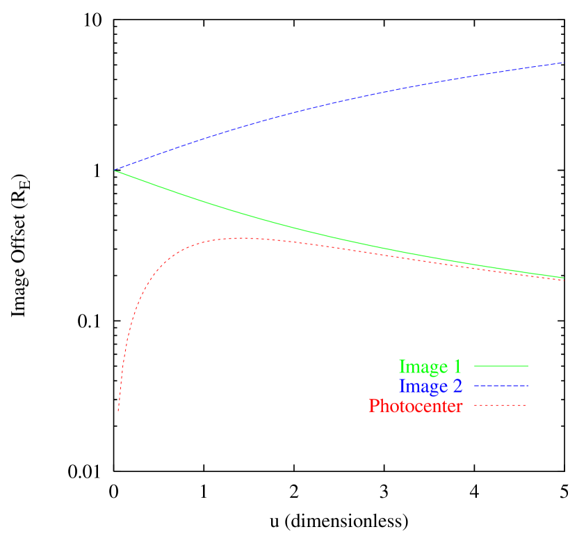
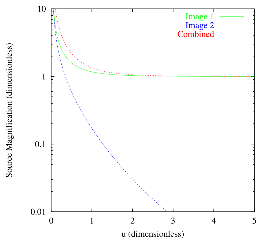
Figure 1: Image positions and intensities for a dark lens. Left: The two image apparent positions and the center-of-light apparent position (in the transverse lens plane) as a function of $u$. Right: image (image 1, image 2, combined) magnifications (dimensionless) as a function of $u$.

2.2 Microlensing Encounter – Barycentric Observer

The geometry of a typical, simple microlensing encounter observed in a barycentric (inertial) system is depicted in Figure 2. The source, lens, and observer are taken as free to move linearly on the time scale of the lensing event. Consequently, viewed in a plane containing the lens and normal to the unperturbed source line-of-sight, the relative source-lens trajectory is approximately linear during the encounter. Without loss of generality we may define a coordinate system in which the source appears stationary and assume that only the lens is in motion. Defining the $x$-$y$ plane of that coordinate system in the transverse lens plane centered on the source (projection), and taking the $x$-coordinate along the trajectory of the lens (see Figure 2), we can write the lens motion in this system as:

$${\bf{x}}_{lens}(t)=\left\{\begin{array}[]{c}v(t-t_{max})\\ -b_{min}\\ \end{array}\right\}$$

with $v$ as the relative lens-source transverse speed, $b_{min}$ as the minimum source-lens impact parameter, and $t_{max}$ the time of (transverse) lens-source closest approach or maximum amplification ($b_{s}=b_{min}$ at $t=t_{max}$). This relative trajectory yields a simple expression for the dimensionless source-lens transverse separation $u(t)$ (and its vectorial counterpart ${\bf u}(t)$):

$$u(t)=\frac{\sqrt{b_{min}^{2}+v^{2}(t-t_{max})^{2}}}{R_{E}} = \sqrt{p^{2}+\frac{(t-t_{max})^{2}}{t_{0}^{2}}}=\sqrt{p^{2}+[t]^{2}}$$

$${\bf u}(t) = {\bf{x}}_{lens}(t)/R_{E}=\left\{\begin{array}[]{c}[t]\\ -p\\ \end{array}\right\}$$ (9)

where we have defined dimensionless minimum impact parameter $p\equiv b_{min}/R_{E}$, the characteristic time or time scale for the microlensing event $t_{0}\equiv R_{E}/v$ – the time required for the lens to move transversely one Einstein radius, and a normalized (dimensionless) time coordinate $[t]\equiv(t-t_{max})/t_{0}$. To predict the time-dependent microlensing observables, $u(t)$ or ${\bf u}(t)$ (Eq. 9) is inserted into the expressions for the combined image light amplification (Eq. 5) and apparent astrometric perturbation (Eq. 2.1). Paczyński 1996a Figure 5 gives sample photometric signature lightcurves for simple microlensing events for several values of the minimum impact parameter $p$. This lightcurve shape is precisely the photometric signature for simple microlensing; current microlensing survey projects (OGLE – Paczyński et al (1995), MACHO – Alcock et al (1996), EROS – Renault et al (1997), DUO – Alard et al 1995b ) first started observing such lightcurves in 1993, and by this time have observed many such lightcurves that agree well with this simple theoretical expectation.

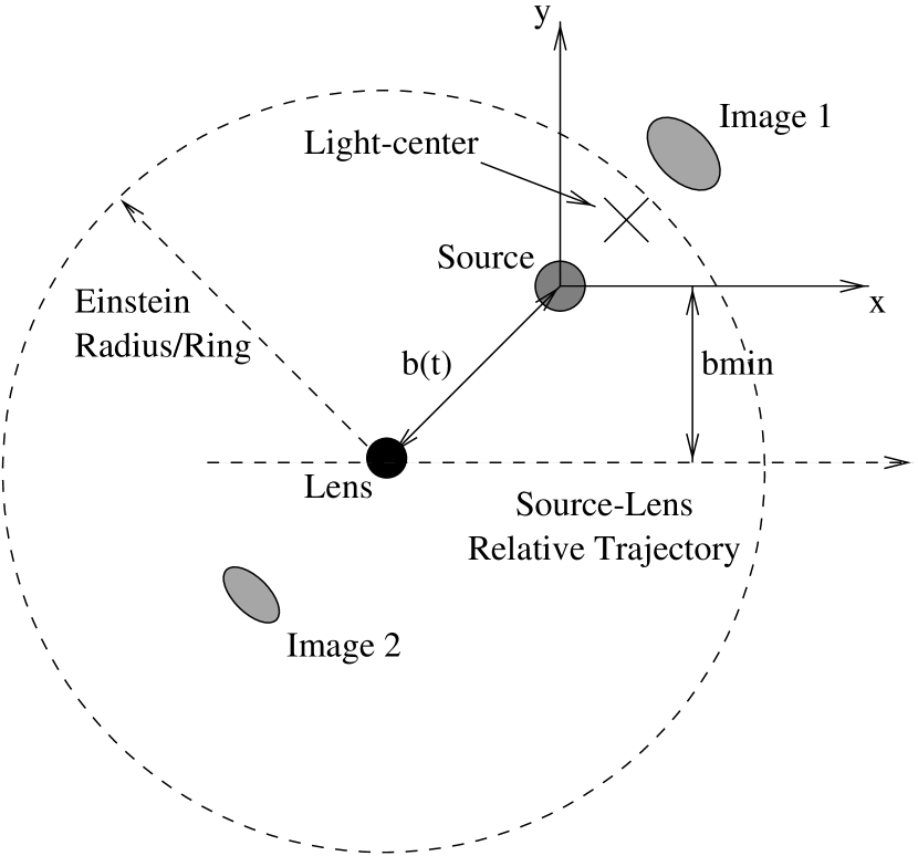
Figure 2: Microlensing encounter geometry. The geometry and differential frame coordinate system of a microlensing event is depicted in a plane normal to the source line-of-sight containing the lens. The relative source-lens trajectory moves from left to right (direction of increasing x), and is parameterized by the lens speed and minimum impact parameter relative to the source.

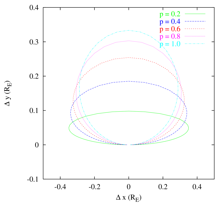
Figure 3: Simple microlensing encounter center-of-light motion. Shown here for a range of sample $p$-values are the motions of the apparent center-of-light position traces relative to the nominal source position for encounter times -20 $\leq[t]\leq$ 20 (Eq. 10). The profiles are elliptical (note the anisotropy of the scale), and are seen to become more eccentric with decreasing $p$-value (Eq. 11).

As seen by the barycentric observer the source apparently performs an elliptical excursion from its unperturbed position (Walker (1995)). The apparent source astrometric excursion is straightforwardly obtained by inserting (the vectorial components of) $u(t)$ (Eq. 9) into $\Delta\theta(u)$ (Eq. 2.1):

$$\Delta{\vec{\theta}}([t])=\frac{R_{E}}{D_{lo}}\;\frac{-{\bf u}([t])}{u^{2}([t])+2}=\frac{r_{E}}{p^{2}+[t]^{2}+2}\left\{\begin{array}[]{c}-[t]\\ p\\ \end{array}\right\}$$ (10)

and depicted in Figure 3 for sample values of $p$ ($p$ = 0.2, 0.4, 0.6, 0.8, and 1). It is likewise straightforward to derive the eccentricity of this excursion in terms of $p$:

$$e=\sqrt{1-\frac{p^{2}}{p^{2}+2}}$$ (11)

The excursions become more eccentric with decreasing $p$, as the maximum intensity of the two images is approximately equal (Eq. 4). The maximum scalar magnitude of the astrometric signature, 2${}^{-3/2}\;r_{E}$, is the same for all photometrically observable ($p\leq 1$) events – it is in fact the same for all events with $p\leq\sqrt{2}$. The angular Einstein radius is given in Figure 4 as a function of lens distance for bulge and LMC microlensing events and a representative range of lens masses ($m$ = 0.05, 0.1, 0.25, 0.5, 1 M_☉). For example, a $m$ = 0.1 M_☉ object at 8 kpc lensing a LMC source has an angular Einstein radius of 3 $\times$ 10^-4 arcseconds or 300 microarcseconds (1 microarcsecond, abbreviated $\mu$as, equals $10^{-6}$ arcseconds) – and a maximum astrometric signature of roughly 100 $\mu$as.

It is noteworthy that the time evolution of the astrometric excursion is non-uniform. Far from lens-source closest approach the apparent source motion is slow, while near the closest approach the source motion is significantly higher. This behavior is depicted in Figure 6 (where points are plotted along the excursion trajectory at equal time intervals), and can be seen by differentiating the astrometric excursion with respect to time:

$$\frac{d\;\Delta\vec{\theta}([t])}{d\;[t]}=\frac{-r_{E}}{(p^{2}+[t]^{2}+2)^{2}}\left\{\begin{array}[]{c}p^{2}-[t]^{2}+2\\ 2p[t]\\ \end{array}\right\}$$ (12)

Clearly for $[t]^{2}\gg p^{2}$ (i.e. far from maximum amplification) the excursion rate magnitude goes as $[t]^{-2}$. This behavior is significant in that the astrometric excursion described in Eqs. 10 and 12 appears very different than the time-harmonic astrometric excursion expected if the source has massive gravitational companions (Lestrade et al (1994); Benedict et al (1995); Gatewood (1996)).

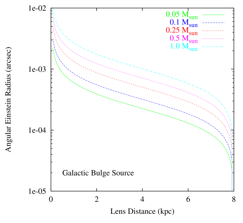
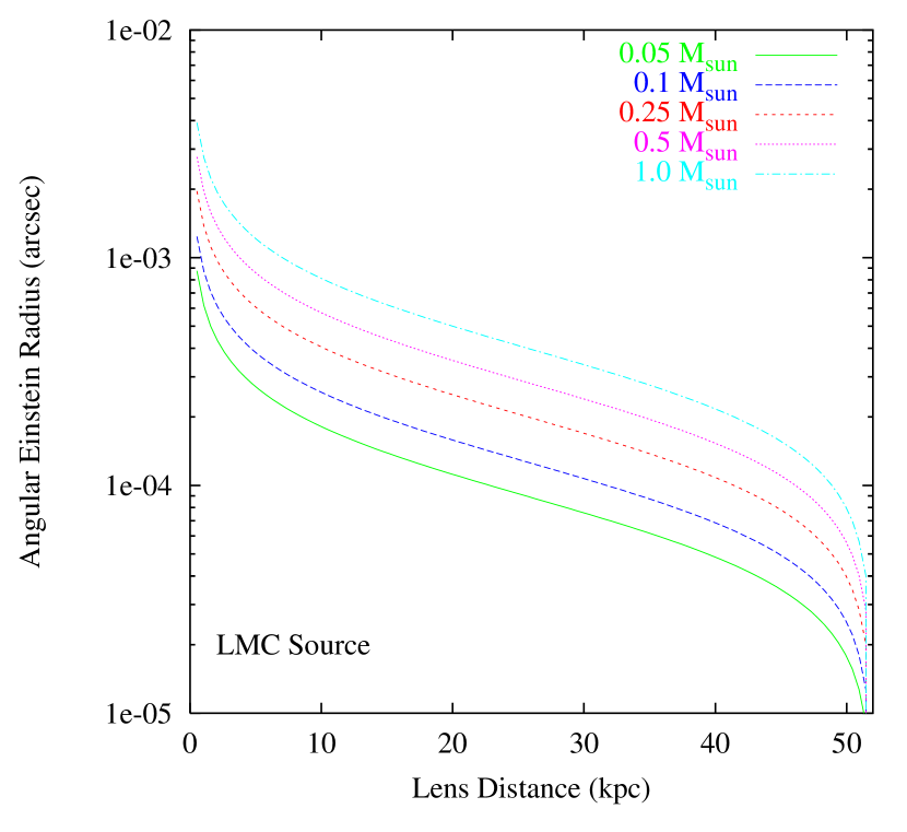
Figure 4: Microlensing Encounter Angular Einstein Radius. Left: the angular Einstein radius ($r_{E}$) for bulge sources as a function of lens distance for lens masses between 0.05 and 1 M_☉ ($m$ = 0.05, 0.1, 0.25, 0.5, 1 M_☉). Right: the same quantity for LMC events. The astrometric signature magnitude for microlensing events is given by 2${}^{-3/2}r_{E}$ $\approx$ 0.35 $r_{E}$. Thus a $m$ = 0.1 M_☉ object at 8 kpc lensing a LMC source has an angular Einstein radius of 300 $\mu$as – and a maximum astrometric signature of roughly 100 $\mu$as.

Finally, it is illustrative to compare the time scales for the photometric and astrometric perturbations caused by a microlensing encounter. Figure 5 plots the photometric amplification and astrometric perturbation magnitude for positive (normalized) encounter times for a $p$ = 0.4 microlensing event. The photometric amplification decays from maximum to nominal level in one single time scale ($t_{0}$). In sharp contrast, the astrometric effects are much more persistent, roughly requiring factors of 30 and 300 more time to decay to 10% and 1% of the maximum astrometric signature respectively. The MACHO collaboration reports a typical time scale $t_{0}$ for a microlensing event to be on the order of one month. Figure 5 makes the point that measurable microlensing astrometric perturbations in events with such a $t_{0}$ will span a period of years – depending on the astrometric sensitivity.

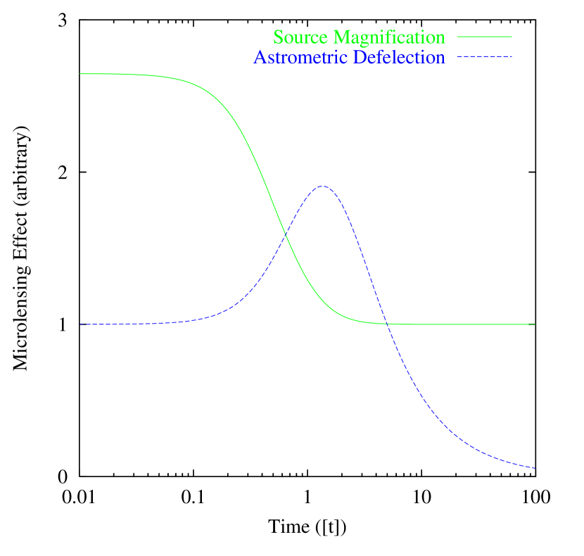
Figure 5: Comparison of Microlensing Astrometric and Photometric Effects. This figure shows the amplification factor and magnitude of the astrometric perturbation as a function of encounter time for an event with $p=0.4$. The photometric amplification is seen to decay from maximum amplification to a nominal value of 1 (no amplification) in roughly 1 event time scale ($t_{0}$). By comparison, the astrometric perturbation (normalized to the perturbation at $t=t_{max}$, $r_{E}\;p/(p^{2}+2)$) increases to its maximum value at $[t]\sim 1$, and then decays to zero in a time scale several orders of magnitude larger than the photometric amplification. If $t_{0}\sim$ 1 month as reported for LMC microlensing events by the MACHO collaboration, measurable astrometric deflections in such events would last over periods of years – depending on astrometric sensitivity.

The case for astrometric observation of microlensing events is both clear and compelling. Barycentric photometric measurements alone constrain the normalized impact parameter $p$ and time scale $t_{0}$ for a microlensing event through Eq. 5 (Paczyński 1996a Figure 5). Astrometric measurements (in lieu of or in addition to photometric measurements) made by a barycentric observer additionally constrain the angular Einstein radius $r_{E}$ and the lens transverse motion direction (orientation of our x-axis) for the microlensing event through Eq. 10. These two quantities taken together are sufficient to compute the (relative) proper motion of the lens object. However, because the distance to the lens is not directly established, no direct inference can be made about $R_{E}$, and thereby the mass and transverse velocity of the lens.

2.3 Microlensing Encounter – Near-Earth Observer

If the microlensing astrometry is observed by an (near) Earth-based instrument over an extended period of time, parallactic effects due to the finite source and lens distances become important as the assumption of linear relative motion in §2.2 is broken by the motion of the observer. Figure 6 depicts an example of astrometric trajectories as viewed by barycentric and terrestrial observers for an arbitrary $p=0.4$ microlensing event. An LMC source is assumed to be lensed by a 0.1 M_☉ lens at 8 kpc ($r_{E}\sim$ 300$\mu$as). It is clear that astrometry sufficient to measure the microlensing astrometric excursion will also observe the relative parallactic motions of the source and lens. So unlike the case of barycentric observations, the distance to the lens (actually, the relative source/lens distance) is accessible by this parallax measurement, and a model-independent estimate of the lens mass and (transverse relative) velocity can be derived. An independent model for source distance and proper motion allows the lens distance and motion to be estimated. A clear case of making virtue from necessity.

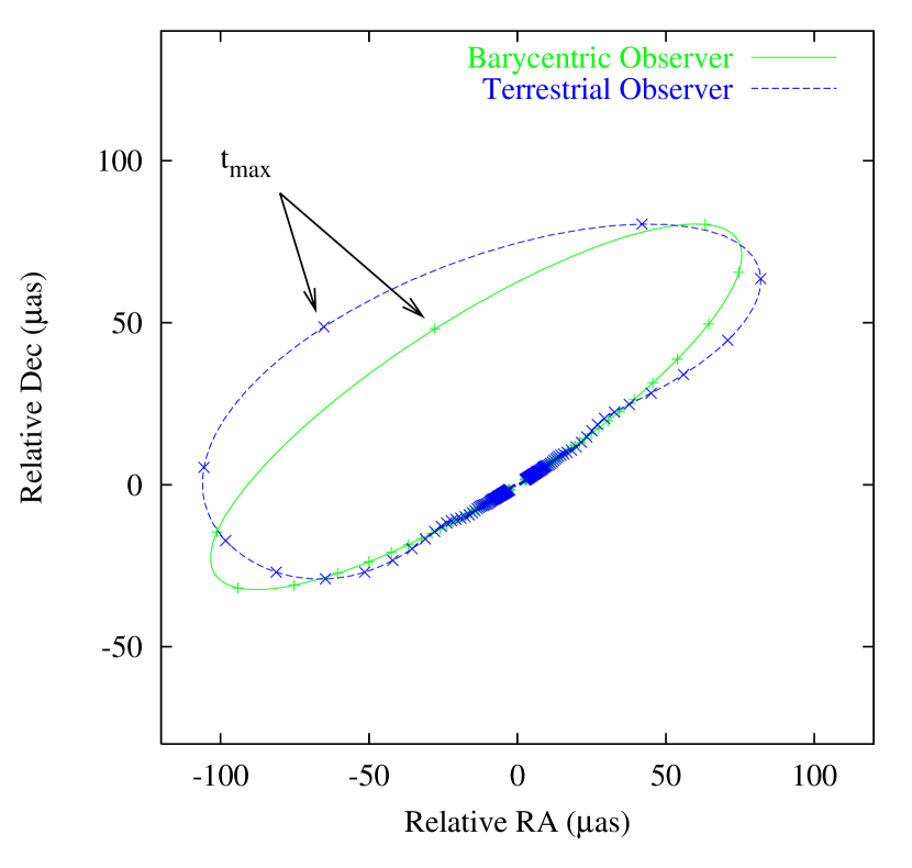
Figure 6: Parallactic Perturbation to Barycentric Microlensing Astrometry. This figure shows the astrometric deflection for a $p=0.4$ microlensing event as viewed by barycentric and terrestrial observers over a period of $\pm$ 50 $t_{0}$ = $\pm$ 5 yr. Marks on the two trajectories are given at $t_{0}$ = 0.1 yr intervals. (The parallactic motion of the background source – 20 $\mu$as – is removed to facilitate comparison.) The background source is taken in the LMC ($D_{so}\sim$ 50 kpc), and the lens is taken to be in the galactic halo ($D_{lo}\sim$ 8 kpc), with an angular Einstein radius of 300 $\mu$as ($m\sim$ 0.1 M_☉). Astrometry sufficient to measure the microlensing perturbation will also measure the parallax effects. A parallax measurement can be used to estimate the relative source/lens distance to the lens, which in turn allows the lens mass, distance, and relative transverse velocity to be inferred for individual events. The time marks corresponding to (barycentric) $t_{max}$ are shown.

An observer at barycentric 3-position ${\bf b}$ (measured in AU) observes an object in barycentric direction ${\hat{\bf n}}_{b}$ to have an apparent parallactic deflection:

$$\pi\left[{\hat{\bf n}}_{b}({\hat{\bf n}}_{b}\cdot{\bf b})-{\bf b}\right]$$

with $\pi$ as the parallax of the source (given in arcseconds by the reciprocal of the distance to the source in parsecs). Both the source and lens are at finite distance, so both acquire parallactic displacements. In the two-dimensional microlensing coordinate system of §2.2, we can write the time-dependent correction to the (normalized) source-lens separation ${\bf u}(t)$ (Eq. 9):

$$\Delta{\bf u}(t) = \frac{\pi_{lens}}{r_{E}}\left[{\hat{\bf n}}_{lens}({\hat{\bf n}}_{lens}\cdot{\bf b}(t))-{\bf b}(t)\right]-\frac{\pi_{source}}{r_{E}}\left[{\hat{\bf n}}_{source}({\hat{\bf n}}_{source}\cdot{\bf b}(t))-{\bf b}(t)\right]$$ (13)

$$\approx \frac{\pi_{lens}-\pi_{source}}{r_{E}}\left[{\hat{\bf n}}({\hat{\bf n}}\cdot{\bf b}(t))-{\bf b}(t)\right]=\frac{\Pi}{r_{E}}\left[{\hat{\bf n}}({\hat{\bf n}}\cdot{\bf b}(t))-{\bf b}(t)\right]$$

assuming ${\hat{\bf n}}_{lens}\approx{\hat{\bf n}}_{source}\approx{\hat{\bf n}}$ ($\delta n/n\sim O(10^{-9})$), defining the relative lens-source parallax $\Pi\equiv\pi_{lens}-\pi_{source}$, and with ${\hat{\bf n}}$ and ${\bf b}$ rotated into the microlensing coordinate system. With this parallactic correction to ${\bf u}(t)$, Eq. 10 predicts the astrometric excursion observed by the terrestrial observer (an example of which is depicted in Figure 6). However, it is important to remember that Eq. 10 refers to the excursion relative to the unperturbed source position, which itself now appears to move with time in an inertial frame due to parallactic effects. This formulation is useful, because, as we will argue below, this observational problem lends itself to narrow-angle differential astrometry techniques.

There are several remarkable points concerning the finite distance correction to the microlensing astrometry. First, as noted above, fitting a model based on Eq. 10 to such astrometric data allows the direct estimate of all the physical parameters for the lens. Strictly speaking, this statement assumes $D_{so}$ and the source proper motion can be separately established (or inferred) by other means. For instance, the distance to the lens (in parsecs) is simply given by:

$$D_{lo}=\frac{D_{so}}{1+D_{so}\Pi}$$ (14)

with $D_{so}$ in parsecs and $\Pi$ in arcseconds. However, the lens mass is a special case in that it can be estimated just from quantities we observe directly, namely $r_{E}$ and $\Pi$. This fact can be seen by inverting Eq. 2 to solve for $m$:

$$m=\frac{c^{2}}{4G}\;\frac{R_{E}^{2}}{D_{so}\;x\;(1-x)}=\frac{c^{2}}{4G}D_{so}r_{E}^{2}\;\frac{x}{1-x}=\frac{c^{2}}{4G}\;\frac{r_{E}^{2}}{\Pi}\;[pc]$$ (15)

where the last equality comes from the fact that $x/(1-x)=1/D_{so}\Pi$ with $D_{so}$ in pc and $\Pi$ in arcseconds. The units of $r_{E}$ are in radians and $\Pi$ in arcseconds, and the $[pc]$ factor is the length of a parsec expressed in the length units of $c$ and $G$ (e.g., meters). The dimensions of Eq. 15 are lacking in elegance, but the result is that we have exchanged the uncertainty in an independent estimate of $D_{so}$ for the uncertainty in the definition of an astronomical unit and the quantities that can be directly measured in a suitable differential astrometric frame. The second interesting point is to note the breaking of the time symmetry around $t_{max}$ by the parallactic correction. Figure 6 demonstrates this point in a particular instance as the barycentric $t_{max}$ time points are labeled on the two excursion trajectories. The degree of symmetry breaking is dictated by the observer’s orbit phase and source position in the sky. In general this parallactic symmetry breaking leads to asymmetric lightcurves and different times for maximum amplification for the barycentric and terrestrial observer, both of which have been noted by other authors (Gould (1992); Hosokawa et al (1993); Miyamoto & Yoshi (1995); Buchalter & Kamionkowski (1996); Gould (1996); Gaudi & Gould (1997)), and has been observed (Alcock et al (1995)).

3 Astrometric Observations

During a microlensing encounter photometric observations alone constrain the impact parameter $p$ and $t_{0}$ through Eq. 5, while microarcsecond-class astrometric observation can be used to uniquely determine the fundamental parameters of the lens (mass, distance, and transverse velocity) without appealing to a lens population model. Strictly speaking, computing the lens distance and transverse velocity requires the source distance and proper motion to be separately established, while the lens mass can be estimated without appealing to the source distance provided the relative parallax between lens and source can be established (Eq. 15). Such a measurement can be made on the basis of differential astrometry provided an astrometric frame in which the background source is quasi-stationary can be established. Currently LMC, SMC, and bulge microlensing events are identified by photometric programs searching rich fields of objects at roughly the same distance as a lensed source. A differential astrometric frame formed from such objects would then have roughly the same parallactic and proper motions as the lensed source, and the apparent source excursion could be measured against this reference to establish $r_{E}$ and $\Pi$. This result is compelling, because while microarcsecond wide-angle astrometry requires a space-based platform (Lindegren & Perryman (1996); Unwin et al (1997)), microarcsecond-class differential astrometry over narrow fields is possible from the ground (Shao & Colavita (1992)). These considerations strongly suggest a program to perform differential astrometry on microlensing candidate events detected in photometric surveys; in such a program the lens mass would be directly determined, and the lens distance would be infered based on a model distance to the source.

It is interesting to investigate the sensitivity that such an astrometric program would produce. To address this question we have constructed a simulation code that creates synthetic photometric and astrometric measurement sets, and then fits a parametric microlensing model to these measurement sets. The measurement synthesis model uses a parametric microlensing model (i.e. lens motion relative position angle, $p$, $r_{E}$, $t_{0}$, $t_{max}$, nominal source amplitude, $\Pi$, nominal source position, and source proper motion in the frame) and specifications of the measurement sequences to simulate (time intervals and measurement frequencies for photometric and astrometric sampling, measurement error model – e.g. the sigmas for the zero-mean gaussian errors applied to the simulated measurements). Then a microlensing model fitting procedure is used to simultaneously fit the synthetic astrometric and photometric datasets and extract estimates of the microlensing event parameters. We have studied parameter estimation performance using both derivative-based (Marquardt least-squares) and derivative-independent (downhill simplex) fitting methods – the results are in good agreement with each other. The simulation code is structured to perform this operation in a Monte Carlo mode, so error distributions in the extracted microlensing parameters may be empirically derived as a function of physical parameters and measurement error models.

Figure 7 shows sample outputs of the synthetic observation and fitting process for an LMC microlensing event. For this example the lens is again assumed to be at distance of 8 kpc ($\Pi$ = 100 $\mu$as), $r_{E}$ = 300 $\mu$as ($R_{E}\sim 2.4$ AU, $m\sim 0.1M_{\sun}$), $t_{0}$ = 0.1 yr (relative lens-source transverse speed of 120 km s^-1), and a lens motion position angle of 30 deg. Operationally we assume the event is detected photometrically, and an astrometric campaign starts – this implies astrometry near and after maximum amplification. Assuming 3% photometry and 10 $\mu$as differential astrometry (the sigmas of the zero-mean gaussian errors added to the measurement sequences) referenced to the unlensed source position, we fit a parametric microlensing model to the combined data set. The fit is seen to reproduce the measurement sets faithfully, and predicts the microlensing parameters accurately. Figure 8 shows the microlensing parameter residuals obtained in 500 instances of the event depicted in Figure 7. In particular, we observe 2% and 16% fractional sample standard deviations on the $r_{E}$ and $\Pi$ residual distributions respectively. (Fitting Gaussian profiles to the central parts of the residual distributions result in error estimates that are $\sim$ 20% better that the sample standard deviations). Using the sample standard deviation figures, the error in estimating the lens mass is 16% in Eq. 15, clearly dominated by the parallax error. Further, if we were to assume a 10% error in estimating the source distance at the LMC, Eq. 14 yields a lens distance accurate to 13%. Such an estimate of the lens distance would unequivocally identify the lens as a member of the galactic halo, and exclude the possibility that the lens was either in the galactic disk or the LMC itself at high confidence (Sahu (1994); Gates et al (1997)).

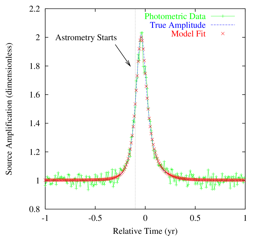
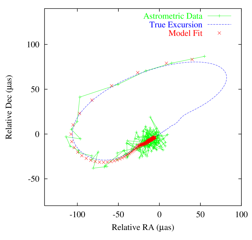
Figure 7: Sample Microlensing Model Fitting. Here we show an example of fitting a microlensing model to synthetic terrestrial photometry and astrometry datasets for a microlensing encounter. The critical parameters for the event are a lens motion position angle of 30 deg, $p$ = 0.4, $r_{E}$ = 300 $\mu$as, and $\Pi$ = 100 $\mu$as ($m$ = 0.1 M_☉). We assume the event is identified photometrically, and differential astrometric measurements commence after that detection. The microlensing model described in §2 was simultaneously fit to both the photometric and astrometric data. Shown in each are the simulated data, true values, and the model fit. Left: the photometric lightcurve results. In this example we assume 3% RMS error photometry. The time units on the $x$-axis are plotted relative to the barycentric $t_{max}$. Once a microlensing interpretation seems likely, we commence astrometric measurement – this time point is shown. Note that the time of maximum amplification for the terrestrial observer is offset relative to a barycentric observer. Further, the lightcurve is slightly asymmetric with respect to the time of maximum amplification. Both of these effects are well known for terrestrial microlensing observation. Right: the corresponding depiction for the astrometry sequence relative to the nominal source position. The simulated 10 $\mu$as RMS error astrometric measurements begin shortly before maximum magnification, and continue for 50 $t_{0}$ after maximum magnification. The true excursion trajectory is shown over the complete excursion, but the microlensing model fit prediction is rendered only for the interval of the astrometric measurements.

Figure 8: Sample Monte Carlo Fit Residual Distributions. Here we show a sample of the microlensing model fit residual distributions obtained in 500 measurement sequence instances taken from the microlensing event depicted in Figure 7. Measurement parameters are the same as discussed in Figure 7: 3% photometry and 10 $\mu$as differential astrometry. Distributions are shown for lens motion position angle (top left), normalized impact parameter (top right), angular Einstein radius (lower left), and relative parallax (lower right). These astrometric experiments are seen to yield fractional uncertainties in the angular Einstein radius and parallax of 2% and 16%, respectively, yielding a 16% error in the lens mass estimate by Eq. 15. Further, combined with a separate model for the source distance (assumed 10% accuracy), the relative parallax estimate preformance yields a 13% estimate for the lens distance, easily sufficient to unequivocally establish its location in the halo.

By Eq. 15, a given mass lens lies along a particular contour in the space of $\Pi$ vs. $r_{E}$. Armed with our event simulation code we have surveyed this $\Pi$ vs. $r_{E}$ phase space of microlensing events for experiment sensitivity to microlensing parameters – with a particular emphasis on the lens mass. Table 1 gives a summary of the set of microlensing and astrometry parameters we considered in our Monte Carlo runs. We ran 500 instances of each parameter permutation given in the table – a total of 384 cases in all. In addition to the parameters specified in Table 1, in each of these experiments we assumed conditions similar to those described above in Figure 7: namely 3% photometry for event detection, and a 5-yr astrometric sequence starting at $t_{max}-t_{0}$, and sampling with uniform period 0.1 $t_{0}$. Microlensing parameter fits are made to the astrometric dataset combined with a 3% photometric dataset that spans the interval $t_{max}\;\pm$ 1 yr. We considered fitting only the astrometry sequence in a few selected cases, but invariably found significantly degraded parameter estimates (similar remarks can be found in Høg et al (1995)).

$r_{E}$	$\Pi$	$p$	$t_{0}$	$\sigma_{ast}$
($\mu$as)	($\mu$as)	-	(yr)	($\mu$as)
100	50	0.4	0.1	5
300	75	0.8	0.2	10
1000	100			25
	200			50
				75
				100
				150
				200

Table 1: Microlensing Monte Carlo Parameter Space. This table gives the set of microlensing and astrometric accuracy parameters we considered in our Monte Carlo runs. We ran a complete set of cases spanning all possible permutations of these parameter values (384 cases in all).

Figure 9 shows the variation of fractional lens mass error vs. astrometric error for three illustrative cases: $r_{E}$ = 100 $\mu$as, $\Pi$ = 50 $\mu$as ($m$ = 0.02 M_☉); $r_{E}$ = 300 $\mu$as, $\Pi$ = 100 $\mu$as ($m$ = 0.1 M_☉); and $r_{E}$ = 1000 $\mu$as, $\Pi$ = 200 $\mu$as ($m$ = 0.6 M_☉). In each of these cases $p$ = 0.4 and $t_{0}$ = 0.1 yr. Here the lens mass error is estimated from the observed uncertainties (residual sample standard deviations) in $r_{E}$ and $\Pi$ (and the generally nonzero covariance). This behavior is suggestive that the mass error scales by a power law of the astrometric error – we find these cases to be typical of the range of Monte Carlo cases considered.

Figure 9: Fractional Mass Error vs. Astrometric Error: Three Examples. Here we show three samples of fractional mass error vs. astrometric error from our ensemble of Monte Carlo results. The three examples are: $r_{E}$ = 100 $\mu$as, $\Pi$ = 50 $\mu$as ($m$ = 0.02 M_☉); $r_{E}$ = 300 $\mu$as, $\Pi$ = 100 $\mu$as ($m$ = 0.1 M_☉); and $r_{E}$ = 1000 $\mu$as, $\Pi$ = 200 $\mu$as ($m$ = 0.6 M_☉). Not surprisingly, we find the fractional mass error to scale as a power law of the astrometric error in all our Monte Carlo results.

Ignoring the correlation term, we can estimate the fractional mass error as a function of the fractional errors in $r_{E}$ and $\Pi$ from Eq. 15:

$${\widehat{\frac{\sigma_{m}}{m}}}\approx\sqrt{\frac{4\sigma_{r_{E}}^{2}}{r_{E}^{2}}+\frac{\sigma_{\Pi}^{2}}{\Pi^{2}}}\approx\sigma_{ast}\;\sqrt{\frac{4}{r_{E}^{2}}+\frac{1}{\Pi^{2}}}$$ (16)

where the second equality comes from crudely estimating the uncertainties in $r_{E}$ and $\Pi$ by $\sigma_{ast}$. Figure 10 shows a scatter plot of the observed fractional mass error from all 384 of our Monte Carlo cases against the estimated fractional error given by Eq. 16. The agreement between the observed and estimated quantities is good, but we find Eq. 16 overestimates the fractional error at large values of $\sigma_{ast}$. A power-law fit to the data indicates that the observed error scales as the estimate in Eq. 16 (hence $\sigma_{ast}$) to the 0.9 power. We attribute this modest sub-linear scaling to the fact that astrometric fits supported by associated photometry resolve $r_{E}$ and $\Pi$ slightly better than the naive estimate of $\sigma_{ast}$. We attribute the observed scatter in the data to the correlation terms which are included in the observed error estimates, but are neglected in Eq. 16. We also note that the $t_{0}$ = 0.2 yr cases on average have lower observed error and smaller scatter than the corresponding $t_{0}$ = 0.1 yr cases. This is not particularly surprising, as the slower time evolution allows for extended observation of the relative parallactic effects.

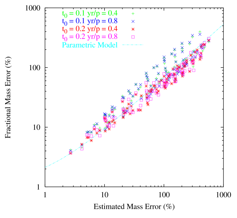
Figure 10: Scatter of Observed Mass Error vs. Estimated Mass Error. Here we show the scatter of the observed fractional mass error vs. the estimated fractional mass error given in Eq. 16. Each data point represents the fractional mass error obtained in 500 instances of measurement sequence fitting. Data sets for $t_{0}$ = 0.1 yr, 0.2 yr and $p$ = 0.4, 0.8 are shown separately – the intrinsic scatter in the $t_{0}$ = 0.2 yr results is noticeably smaller. The data are seen to correlate reasonably well with the crude mass estimate of Eq. 16, but it overestimates the mass error at larger values. A simple parametric fit shows the observed fractional mass error to scale (with moderate scatter) to the estimated fractional mass error to the 0.9 power. We attribute the scatter in the data to the correlation in errors included in the observed error calculation but explicitly ignored in Eq. 16.

Finally, we have argued for and simulated differential astrometric experiments where we assume astrometry in a frame where the source is stationary. This reference frame must be established by observing field objects near the nominal source position. For LMC, SMC, and bulge events where there are many objects at small $\delta D/D$ with the source, the reference frame will absorb common parallactic motions. However, there will be residual frame drifts and rotations resulting from unknown velocity dispersion among the reference objects (and source). The residual linear frame drifts are large (mas yr^-1) on the scale of the microlensing astrometric excursion. The frame rotations will be small (O($10^{-4}$) rad yr^-1), but to the extent that the source is not at the center of the astrometric frame this too adds an effective linear drift to the differential frame of order 100 $\mu$as yr^-1. So in practice the microlensing fit process must account for linear frame drifts that are large compared with the scale of the microlensing excursion. It is straightforward to extend the microlensing parameter model to include a frame drift. Figure 11 gives an example of allowing for a random drift in the astrometric frame, and using an extended microlensing model to solve for this quantity. The physical parameters of the microlensing event in Figure 11 are the same as those used in Figure 7: $r_{E}$ = 300 $\mu$as, $\Pi$ = 100 $\mu$as, $t_{0}$ = 0.1 yr; and we have taken 50 $\mu$as astrometry. To this we have added 1.5 mas yr^-1 of frame drift in a random orientation to the lens motion. The microlensing fit does an acceptable job of identifying the frame drift, bolstered by the time base of astrometry at late encounter times (not shown in the figure). We do not find a coupling between frame drift and the quantities of interest in determining the lens mass: $r_{E}$ and $\Pi$. We have added random frame drifts to several of the Monte Carlo cases described in Table 1, and find that such drifts do not significantly effect our simulation results. This is reasonable, as both $r_{E}$ and $\Pi$ are estimated from the curvature of the astrometric path.

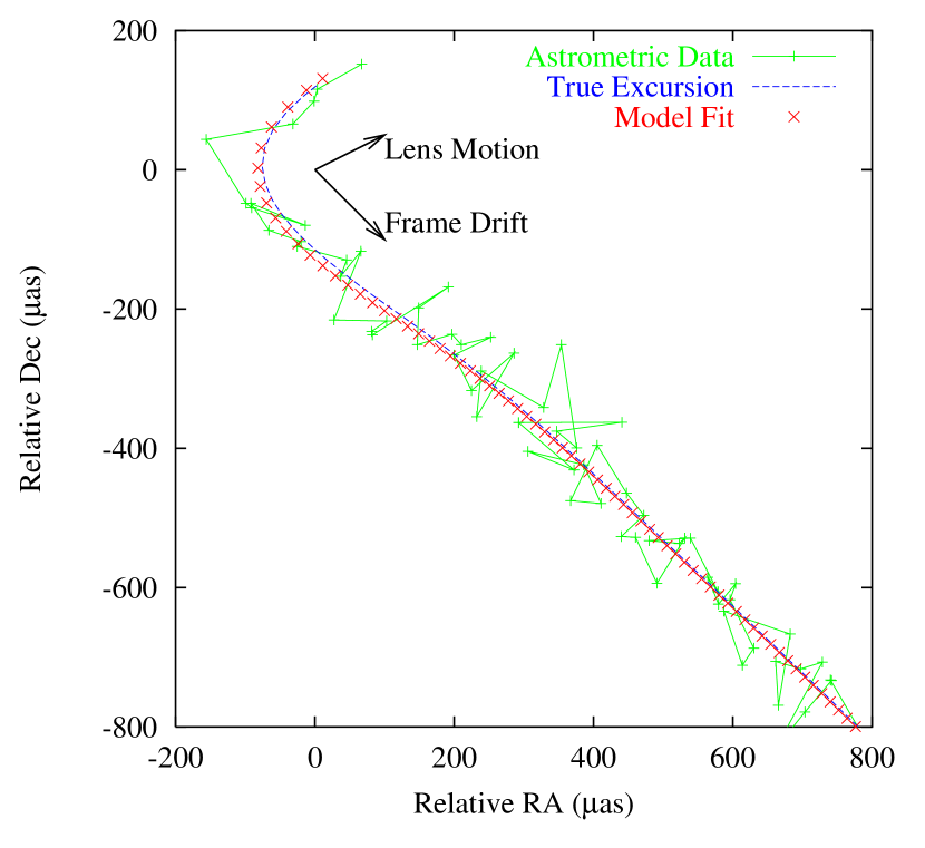
Figure 11: Microlensing Astrometric Fit With Frame Drift. Shown is the result of an astrometric experiment where we have added a linear drift into the differential astrometric frame. The microlensing parameters of this event are the same as used in Figure 7: $r_{E}$ = 300 $\mu$as, $\Pi$ = 100 $\mu$as, $t_{0}$ = 0.1 yr; and we have taken 50 $\mu$as astrometry. We added 1.5 mas yr^-1 of frame drift in a random orientation to the lens motion (vectors indicating the frame drift and lens motion direction are shown). The microlensing fit does an acceptable job of identifying the frame drift. We do not find a coupling between frame drift and the quantities of interest in determining the lens mass: $r_{E}$ and $\Pi$. We have added random frame drifts to several of the Monte Carlo cases described in Table 1, and find that such drifts do not effect our simulation results.

4 Summary and Discussion

We have specialized the Miyamoto and Yoshi suggestion to measure the astrometry of the lensing event photocenter. We agree with their conclusions: that high-precision astrometric observation of MACHO microlensing events hold the promise of determining fundamental lens parameters (mass, proper motion, transverse velocity) in a model-independent fashion. We maintain that it is sufficient to measure the motion of the center-of-light. In particular, in many cases accurate differential astrometry is sufficient obtain the lens mass without additional assumptions (in slight contrast to the earlier suggestion by Walker (1995), who ignored the value of parallactic effects), and reasonable lens distance and transverse velocity estimates can be obtained from an independent model of source distance and proper motion. Such narrow-angle differential astrometry is possible from the ground (Shao & Colavita (1992)). Alternatively, wide-angle microarcsecond-class astrometry can simultaneously determine the source and lens position and kinematic parameters without external information, and again the lens mass. Clearly the potential for probing the physical parameters of the putative halo object population by astrometric techniques is enormous.

A program to probe microlensing events photometrically detected in the galactic bulge seems plausible for the planned Keck Interferometer (KI – Keck Interferometer Project (1997)). KI requires a bright guide star to track atmospheric fluctuations of the interferometric fringes. The brightest bulge objects are 16th magnitude, within the fringe tracking capabilities for the two 10 m apertures. The expected 10 – 20 $\mu$as astrometric performance of KI yields microlensing parameter estimates sufficient to constrain lens mass and distance parameters for individual events, which will give profound insight into the nature of these objects.

However, events in the LMC or SMC are not detectable from the Keck site, both because of geography and sensitivity. The brightest objects in the LMC are 17–18 magnitude, arguably fainter than the tracking capabilities of the KI. However, the declination of these fields would require KI zenith angles that severely degrade the astrometric performance. A large aperture astrometric interferometer in the Southern hemisphere such as the VLT interferometer (VLTI – von der Lüthe et al (1994)) could measure Magellenic cloud events, and in particular determine the lens mass and distance with sufficient accuracy to resolve many of the current issues regarding their nature. Such measurements would be very challenging but are clearly very compelling.

A number of authors have specifically suggested the application of planned space-based global astrometric techniques to analyze these events (Høg et al (1995); Miyamoto & Yoshi (1995); Paczyński (1998)). In space-based applications astrometric references can be drawn from a global astrometric frame tied to extragalactic objects, and the positions, proper motions, and parallaxes of these references are known to a few microarcseconds in a quasi-static frame. Thus the necessity of establishing a narrow-angle relative frame for differential astrometry is removed. Further, astrometry at late times identifies the source proper motion and parallax in the global frame – thereby establishing the source motion and distance. With the source distance and kinematics established, the lens parameters are all uniquely determined. Assuming ground-based observations measure lens masses and distance in the manner we describe, we believe the role of space-based microlensing astrometry programs by planned astrometric space missions such as SIM (Unwin et al (1997)) and GAIA (Lindegren & Perryman (1996)) will be in probing the precision positions and particularly kinematics of the lensing objects. If ground-based measurements of Magelenic cloud events are not possible, then SIM and GAIA seem well-suited to offer definitive answers on the nature of the lenses.

Finally, in the near future it is possible that CCD-based astrometry could make detections of microlensing astrometric perturbations, and possibly make rough estimates of lensing parameters, and/or breaking some of the degeneracies in photometric microlensing observations (see below). Pravdo and Shaklan (Pravdo & Shaklan (1996)) report night-to-night astrometric repeatability of 200 $\mu$as in data taken at the Palomar 5 m telescope, and speculate that limits might approach 100 $\mu$as at the 10 m Keck Telescope. In further assessing these prospects we anxiously await the results of several nights of Keck observations recently made by Pravdo and Shaklan (Shaklan (1997)).

One of the key assumptions we have made in this work is the assumption of a dark lens. This assumption is plausible given the success photometric programs have had in fitting dark lens amplification models to photometric data. However, the instance of a luminous lens is possible and interesting (Miralda-Escudé (1996); Paczyński 1996b ), and the astrometric model derived here can be augmented in a straightforward way. Figure 12 shows an example of a fit to a dataset generated with a luminous lens model unresolved from the lensed source. The physical parameters (bulge event, 10 kps source / 5 kpc lens distance, 0.1 M_☉ lens, lens/source brightness ratio of 0.1) were selected to be comparable to the example given in Figure 7. The model fit faithfully reconstructs the input physical parameters, including the correct attribution of source and lens brightness. One operational question that arises is how does one determine whether a dark lens model is appropriate for a given microlensing event. While one could straightforwardly test the luminous lens hypothesis by adding a relative source/lens luminosity parameter to the microlensing fit model as presented here, a more obvious and compelling resolution to this question is contained in the possible chromaticity of the astrometric observables as described in Eq. 2.1. If the lens is luminous, then its spectral content is in general different from that of the source – implying that both the photometric and astrometric observables will be functions of wavelength. Making the observations in a variety of spectral bands will identify the relative source-lens intensity and color, and provide the necessary data to robustly extend the microlensing model to the general case of luminous lenses. We defer a more systematic analysis of the luminous lens case to future work.

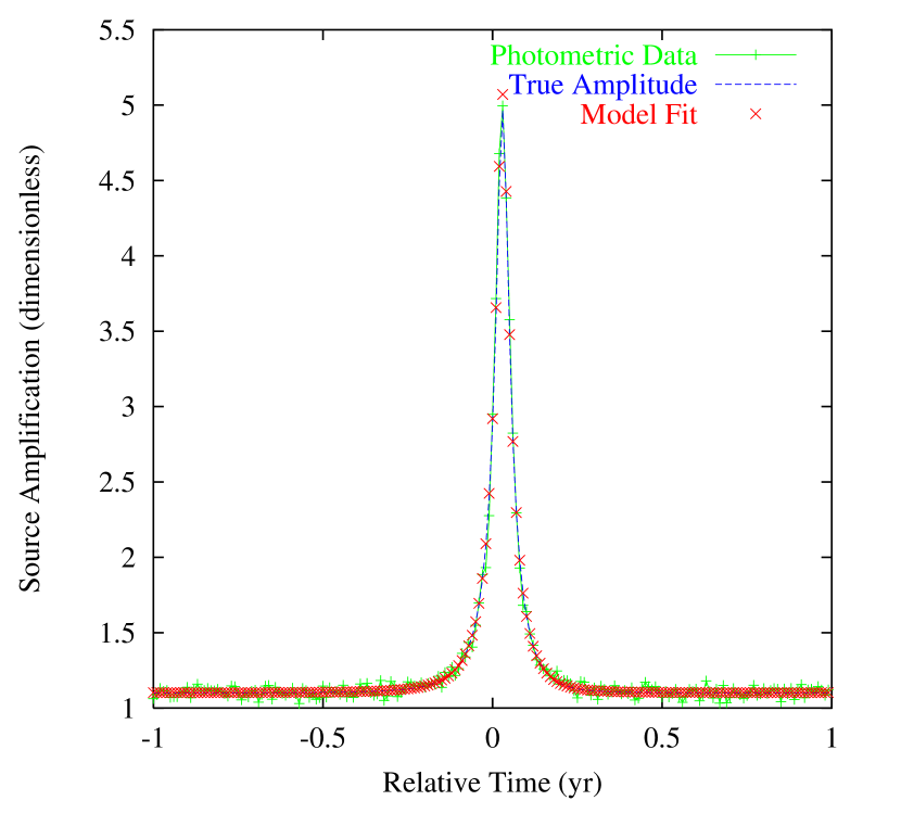
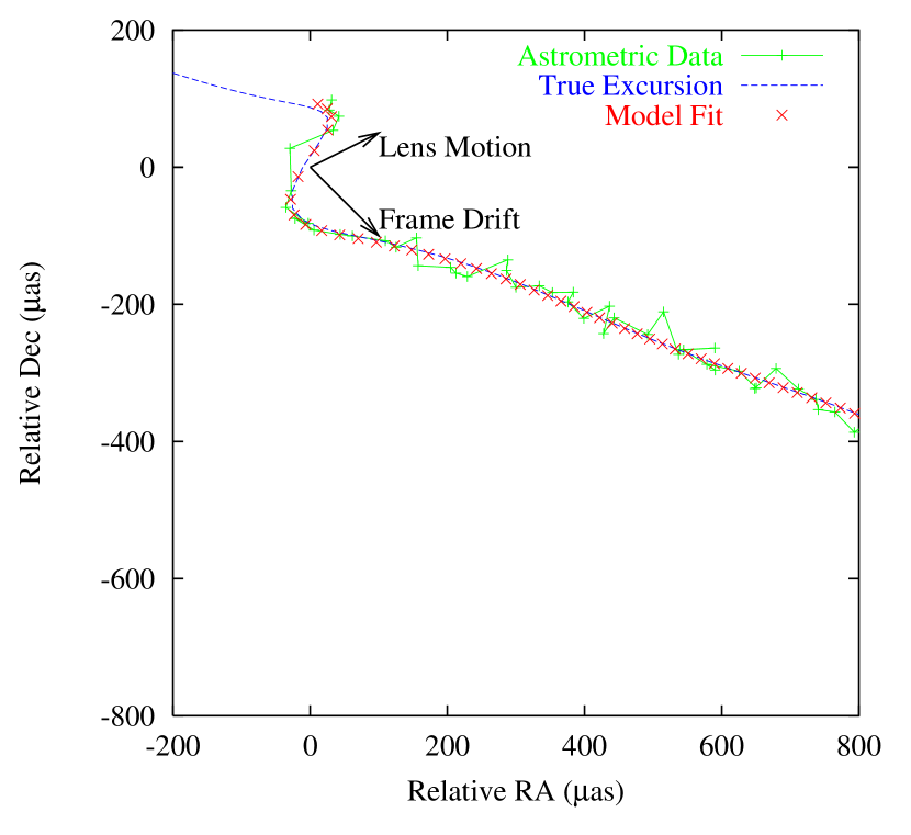
Figure 12: Luminous Lens Microlensing Model Fitting. Here we show an instance of fitting a microlensing model with an unresolved luminous lens to synthetic terrestrial photometry and astrometry datasets for a microlensing encounter similar to that shown in Figure 7. The parameters for the event are a lens motion position angle of 30 deg, $p$ = 0.4, $r_{E}$ = 290 $\mu$as, and $\Pi$ = 100 $\mu$as ($m$ = 0.1 M_☉) and a lens/source brightness ratio of 0.1. Again, we assume the event is identified photometrically, and differential astrometric measurements commence after that detection. The microlensing model described in §2 including a parameter for the relative lens/source brightness was simultaneously fit to both the photometric and astrometric data. Shown in each are the simulated data, true values, and the model fit. Left: the photometric lightcurve results. In this example we assume 3% photometry error. The time units on the $x$-axis are plotted relative to the barycentric $t_{max}$. Right: the corresponding depiction for the astrometry sequence relative to the nominal source position. The simulated 20 $\mu$as astrometric measurements begin shortly before maximum magnification, and continue for 30 $t_{0}$ after maximum magnification. The fit is seen to faithfully reproduce the simulated datasets, and converge to the input model values including the appropriate source and lens brightness, even in the presence of frame drift.

The closely related problem of image blending is discussed in recent work by Alard (Alard (1996)), and Woźniak & Paczyński (Woźniak & Paczyński (1997)), who consider the possibility that a second source (possibly unrelated to either source or lens) is unresolved from the image. Woźniak & Paczyński find that the degeneracies in photometric observation of such events result in systematic errors in estimating lensing parameters. Based on our preliminary successes in correctly distinguishing source and lens luminosities, we concur with the speculation put forward by Woźniak & Paczyński that multi-spectral astrometry and photometry breaks the degeneracy in (some subset of) blended events, and point this out as a particularly important case for future study.

Astrometric Detections – Non-MACHO Events

A number of authors have suggested to broaden the applicability of the astrometric techniques to generic microlensing events (Hosokawa et al (1993); Miralda-Escudé (1996); Paczyński 1996b ; Paczyński (1998)). These events could potentially be detected astrometrically in programs that concentrated on high proper motion objects (so as to sweep-out larger solid angles), or as a part of broader companion search program (something we have integrated into our PTI program – Colavita et al (1994)). While much of the phenomenology we have developed in §2 is directly applicable, there is a practical difficulty in establishing lensing parameters in such events by differential means. The first is the absence of a ready supply of reference objects that share common parallactic motions as the source. The fact that the rich LMC, SMC, and bulge fields used in the photometric surveys naturally yield an abundance of reference objects for which $\delta D/D$ is small makes events in these fields unique. Without such a common parallactic reference, the systematic errors in the determination of $\Pi$ will be too large to establish a precise lens mass from ground-based differential astrometry. Such events would seem to be best studied by space-based, global astrometric techniques.

Complex Lenses

While the majority of photometrically detected events are consistent with single lens hypothesis, a number of binary lens events have been reported (Udalski et al (1994); Alard et al 1995a ; Bennett et al (1996)). In a recent preprint Dominik (Dominik (1997)) argues that photometry alone does not uniquely constrain the binary lens parameters. We speculate that additional astrometric information would break the degeneracies among various hypotheses in binary lens events through straightforward extensions of the astrometric theory developed here. We defer the analysis of the binary lens case to future work.

References

- (1) Alard, C., Mao, S., Guibert, J. 1995, A&A 300, 17 (astro-ph/9506101).
- (2) Alard, C. et al (the DUO collaboration) 1995, Msngr 80, 31.
- Alard (1996) Alard, C. 1996, A&A in press (astro-ph/9609165).
- Alcock et al (1995) Alcock, C. et al (the MACHO collaboration) 1995, ApJ 454, L125 (astro-ph/9506114).
- Alcock et al (1996) Alcock, C. et al (the MACHO collaboration) 1997, ApJ 486, 697 (astro-ph/9606165).
- Benedict et al (1995) Benedict, G.F. et al 1995, BAAS 187, #70.11.
- Bennett et al (1996) Bennett, D.P. et al (the MACHO collaboration) 1996, Nucl. Phys. Proc. Suppl. 51B, 152 (astro-ph/9606012).
- Buchalter & Kamionkowski (1996) Buchalter, A. and Kamionkowski, M. 1996, ApJ 469, 676 (astro-ph/9604144).
- Colavita et al (1994) Colavita, M.M. et al 1994, Proc. SPIE 2200, 89.
- Dominik (1997) Dominik, M. 1997, preprint (astro-ph/9703003).
- Gates et al (1997) Gates, E.I., Gyuk, G., Holder, G.P., and Turner, M.S. 1997, ApJ submitted (astro-ph/9711110).
- Gatewood & De Jonge (1995) Gatewood, G., and De Jonge, J.K. 1995, ApJ 450, 364.
- Gatewood (1996) Gatewood, G. 1996, BAAS 188, #40.11.
- Gaudi & Gould (1997) Gaudi, B., and Gould, A. 1997, ApJ 477, 152 (astro-ph/9601030).
- Gould (1992) Gould, A. 1992, ApJ 392, 442.
- Gould (1996) Gould, A. 1996, PASP 108, 465G (astro-ph/9604014).
- Høg et al (1995) Høg, E., Novikov, I.D., and Polnarev, A.G. 1995, A&A 294, 287.
- Hosokawa et al (1993) Hosokawa, M., Ohnishi, K., Fukushima, T., and Takeuti, M. 1993, A&A 278, L27.
- Keck Interferometer Project (1997) Keck Interferometer Project 1997 http://huey.jpl.nasa.gov/keck
- Lestrade et al (1994) Lestrade, J.F., Jones, D., Preston, R., and Phillips, R. 1994, Ap&SS 212, 251.
- Lindegren & Perryman (1996) Lindegren, L. and Perryman, M.A.C. 1996, A&AS 116, 579L.
- von der Lüthe et al (1994) von der Lüthe, O., Ferrand, D., Koehler, B., Neng-hong, Z., and Reinheimer, T. 1994, Proc. SPIE 2200, 168.
- Miyamoto & Yoshi (1995) Miyamoto, M. and Yoshi, Y. 1995, AJ 110, 1427.
- Miralda-Escudé (1996) Miralda-Escudé, J. 1996, ApJ 470, L113 (astro-ph/9605138).
- Monet et al (1992) Monet, D.B. et al 1992, AJ 103, 638.
- (26) Paczyński, B. 1986a, ApJ 301, 503.
- (27) Paczyński, B. 1986b, ApJ 304, 1.
- Paczyński et al (1995) Paczyński, B. et al (the OGLE collaboration) 1995, BAAS 187, #14.07
- (29) Paczyński, B. 1996a, ARA&A 34, 419 (astro-ph/9604011).
- (30) Paczyński, B. 1996b, Acta Ast. submitted (astro-ph/9606060).
- Paczyński (1998) Paczyński, B. 1998, ApJ 494, L23 (astro-ph/9708155).
- Perryman et al (1997) Perryman, M.A.C. et al 1997, A&A 323. L49.
- Pravdo & Shaklan (1996) Pravdo, S.H. and Shaklan, S.B. 1996, ApJ 465, 264.
- Refsdal (1964) Refsdal, S. 1964, MNRAS 128, 295.
- Renault et al (1997) Renault, C. et al (the EROS collaboration) 1997, A&A 324, L69 (astro-ph/9612102).
- Sahu (1994) Sahu, K.C. 1994, PASP 106, 942 (astro-ph/9408047).
- Shaklan (1997) Shaklan, S.B. 1997, private communication.
- Shao & Colavita (1992) Shao, M., and Colavita, M. 1992, A&A 262, 353.
- Udalski et al (1994) Udalski, A. et al (the OGLE collaboration) 1994, ApJ 436, L103 (astro-ph/9407084).
- Unwin et al (1997) Unwin, S., Boden, A., and Shao, M. 1997, Proc. STAIF, AIP Conf. Proc. 387, 63.
- Walker (1995) Walker, M.A. 1995, ApJ 453, 37.
- Woźniak & Paczyński (1997) Woźniak, P. and Paczyński, B. 1997, ApJ 487, 55 (astro-ph/9702194).
- Zhao (1997) Zhao, H-S. 1997, MNRAS submitted (astro-ph/9703097).