Complex Velocity Fields in the Shell of T Pyxidis

Abstract

We present spatially-resolved, moderate-resolution spectrophotometry of the recurrent nova T Pyx and a portion of the surrounding shell. The spectrum extracted from a strip of width $10^{\prime\prime}$ centered on the star shows well-known, strong emission lines typical of old novae, plus a prominent, unfamiliar emission line at $\lambda$6590. This line, and a weaker companion at $\lambda$6540 which we also detect, have been previously reported by Shahbaz et al., and attributed to Doppler-shifted H$\alpha$ emission from a collimated jet emerging from T Pyx. We demonstrate that these lines are instead due to [N II] $\lambda\lambda$6548, 6584 from a complex velocity field in the surrounding nebula. The comments of past workers concerning the great strength of He II $\lambda$4686 in T Pyx itself are also reiterated.

1 INTRODUCTION

The recurrent nova T Pyxidis was discovered by Leavitt (1914); a history of the object, and some recent observations, may be found in Webbink et al. (1987) and Shara et al. (1989). A compact ($\sim 10^{\prime\prime}$) nebula surrounding the star is described by Duerbeck & Seitter (1979) and Williams (1982), and a larger, fainter shell is observed by Shara et al. (1989). Hubble Space Telescope imagery of the T Pyx nebula (Shara et al. 1997) reveals an exceptionally complex, clumpy structure on subarcsecond spatial scales, and the brightness of at least some of these knots varies on timescales of months. As pointed out by these authors, the HST data vividly demonstrate that “shell” is a quite misleading term for the extended structure near T Pyx, which in fact consists of literally thousands of discrete lumps, most bright in [N II] emission.

Recently an interesting spectrum of T Pyx has been presented by Shahbaz et al. (1997). They call attention to a strong, unfamiliar emission line at $\lambda 6593$, and a weaker feature at $\lambda 6539$. They interpret these features as Doppler-shifted H$\alpha$ lines from a collimated jet emerging from T Pyx, at velocities of +1400 and $-1100$ km s^-1. As there is no a priori reason to expect these particular velocities, and no second spectral feature to confirm them, care must obviously be taken when accepting this interpretation; virtually any unidentified emission line, regardless of wavelength, can be attributed to such a model. Nonetheless this interpretation if correct is very exciting: as stressed by Shahbaz et al. (1997), this would make T Pyx the first short-period cataclysmic variable with a jet. Livio (1998), who comments that “jet lines have now been observed unambiguously in the recurrent nova T Pyx,” stresses that there would be profound implications on models of jet formation.

In an effort to clarify this unprecedented interpretation, we obtained further spectra of T Pyx and the surrounding nebula. Although we verify the existence of the unusual emission lines, the features unfortunately prove to have a less exotic origin than that suggested by Shahbaz et al.

2 OBSERVATIONS AND INTERPRETATION

On UT 1997 December 6, we obtained spectrophotometry of T Pyx with the 3.5-m telescope of the Astrophysical Research Consortium, located at Apache Point, NM, using the Double Imaging Spectrograph (DIS) in its high-resolution mode. In this configuration, DIS simultaneously provides two spectra, each of about 1000 Å coverage in disjoint wavelength ranges, split by a dichroic mirror onto two CCDs. A slit measuring $1\mbox{${}^{\prime\prime}\mskip-7.6mu.\,$}5$ $\times\ 5^{\prime}$ was employed; the measured FWHM of comparison arc lines indicates that a spectral resolution of $\sim 2.4$ Å was achieved. The slit was oriented E/W, passing through the star as well as a series of the bright knots in the nova shell located within a few arcsec of the central object (Shara et al. 1997).

At $\delta=-32^{\circ}$, T Pyx is not well-located for observation from Apache Point, so observations were confined to two hours centered on the meridian. A total of 6600 s of integration in 6 separate exposures was obtained, and the data summed together for analysis. Approximate flux calibration was achieved via observation of spectrophotometric standard stars from Massey et al. (1988) and Massey & Gronwall (1990). However at these large airmasses, the combination of differential refraction and uncertain light losses at the slit are such that these absolute fluxes cannot be regarded as more accurate than $\pm 0.5$ mag.

The two resulting spectra appear in Figure 1. Strong Balmer and He I emission are evident, as is typical in many old novae, as well as the prominent C III/N III $\lambda\lambda 4640,4650$ blend and especially He II $\lambda$4686. The spectrum is similar to that displayed by Williams (1983) and described by Duerbeck & Seitter (1987). We reiterate the remarks by Williams (1983) and Williams (1989) concerning the great strength of He II $\lambda$4686, which equals or exceeds H$\beta$ in intensity. As this latter circumstance is usually seen only in magnetic cataclysmic variables, the polarization properties of T Pyx are clearly of great interest and should be determined. Because the extraction width of the data in Figure 1 is $10^{\prime\prime}$, the stellar Balmer and He II emission may also contain a component due to the surrounding nebula. Low resolution spectral scans of the north portion of the nebula, uncontaminated by the star but spatially disjoint from the region observed in this work, by Williams (1982) show a quite small value of $\lambda$4686/H$\beta$, hinting but certainly not proving that the unusual ratio seen in the star is truly a valid measure.

Immediately evident in the red spectrum is a prominent, resolved emission line centered at $\lambda$6590, which includes the unusual feature discovered by Shahbaz et al. (1997), and termed “S⁺” by those authors. It is not obviously visible in the lower-resolution data of Williams (1983). In Figure 2 we present intensity contour maps of portions of the spectra displayed in Figure 1, but with the stellar continuum subtracted. Here we also include the spatially-resolved data in the region $\pm 10^{\prime\prime}$ from T Pyx, twice the areal coverage of Figure 1. In these maps, the abscissa is wavelength, and the ordinate is the spatial direction E/W of the central star. Even with the modest pixel scale of DIS ($0\mbox{${}^{\prime\prime}\mskip-7.6mu.\,$}61$ pix^-1 in the red, and $1\mbox{${}^{\prime\prime}\mskip-7.6mu.\,$}1$ pix^-1 in the blue), it is clear that substantial flux is detected in our data from the nebula, spatially resolved from the central star.

Although extensive dispersive nebular spectroscopy of T Pyx has not to our knowledge been presented, it is evident from the work of Williams (1982) and Shara et al. (1989, 1997) that [N II] $\lambda$6584 is very prominent in the knots of the nebula. In agreement with this past work, examination of the contours in Figure 2 readily shows that we have also detected [N II] $\lambda$6584, together with associated [N II] $\lambda$6548, H$\alpha$, and [O III] $\lambda\lambda$ 4959, 5007 emission, at a number of separable, discrete velocities (presumably each corresponding to one or a small number of bright nebular knots) within a few arcseconds of T Pyx.

Interpretation of these data in a two-dimensional plane such as that of Figure 2 can be confusing, as distinct spatial regions can overlap in projection, and velocity differences of $\sim 10^{3}$ km s^-1 can result in the wavelength blending of H$\alpha$ and the two red [N II] lines in one knot with different components of this same triple of lines from other, discrete velocity systems of another knot. To aid in identification of the strongest, most prominent velocity systems, we place on Figure 2 colored bars at the location of [O III] $\lambda\lambda$ 4959, 5007, H$\alpha$, and [N II] $\lambda\lambda$6548, 6584, using a distinct color for each of five identified velocity systems which are prominent. Further velocity structure is evident, but more sophisticated representations of the results are probably not warranted by the relatively crude spectral and spatial resolution of our data. In any case, this analysis suffices to illustrate our most important conclusions. While we have included the appropriate heliocentric correction of $\sim 20$ km s^-1, the absolute velocity calibration of the spectrograph is uncertain at the level of $\sim 10$ km s^-1; relative velocities should be more reliable. A slight additional complication is that due to differential refraction at this high airmass, the red and blue sides of the spectrograph are observing slightly different, although spatially adjacent, regions of the nebula separated by $\sim 1^{\prime\prime}$ (Filippenko 1982); this small effect has no impact on the conclusions reached here.

We first call attention to the “orange” system, at $v\sim+250$ km s^-1. This is very clearly nebular gas, detected simultaneously in five separate emission lines (four of them forbidden) at a consistent velocity, and colocated $3-6^{\prime\prime}$ W of the star. Now consider the nearby “red” system, which lies essentially coincident with the stellar image in the E/W direction. Figure 2 identifies the emission at $\lambda$6595 as [N II] $\lambda$6584 at $v\sim+490$ km s^-1. For this velocity, [N II] $\lambda$6548 and H$\alpha$ are blended with the “purple” and “blue” systems, blue-shifted gas which probably falls only in projection, rather than spatial coincidence, on our image. However, note that the “red” system does appear as expected in [O III] $\lambda$4959 (and cannot be expected to appear in [O III] $\lambda$5007 due to a precise overlap with the strong He I $\lambda$5015 from the star). Furthermore, although it may be a projection effect, the most straightforward interpretation of the orange and red systems is that as they are reasonably adjacent in both velocity and E/W location, they are in fact physically adjacent in the nebula, and both are emission systems from knots in the shell.

Figure 2 shows clearly that in our data the [N II] $\lambda$6584 emission from the orange and red systems combine to form the prominent, spectrally-resolved “S⁺” emission line at $\lambda$6590. Although Shahbaz et al. (1997) do not provide details of the shape and size of the slit or aperture used to obtain their data, and in any case post facto reconstruction of the precise pointing location and seeing is probably not possible, we suggest that the “S⁺” described by these authors is also red-shifted [N II] $\lambda$6584 from knots in the nebula, either physically close to, or seen in projection close to, T Pyx. Indeed, inspection of Figure 2 shows that a narrow, on-axis aperture would produce emission centered at $\lambda 6593$, exactly as they have reported.

We believe that a similar explanation applies to the $\lambda$6539 “S^-” emission line reported by Shahbaz et al., and again attributed by them to H$\alpha$ emission from a collimated jet emitted by the star. We also detect this line, which we denote as the “violet” system in Figure 2. We suggest that the “S^-” line is in fact [N II] $\lambda$6548 at $v=-440$ km s^-1. As this system is spatially projected very close to the star, other lines at the same velocity are difficult to discern, but are indeed present. For example, the corresponding [N II] $\lambda$6584 and [O III] $\lambda$5007 lines in the violet system do appear as intensity peaks at the correct wavelengths, superposed on the stellar continuum, and are visible in Figure 2 as excess contours.

Figure 2 illustrates that even given our meager data at one slit position angle, the velocity structure of the nebula is clearly complex. Shara et al. (1997) have demonstrated that the very small scale spatial structure of the knots is exceptionally intricate, and that knot intensities can fade and grow on a timescale of months. Taken together this implies that ground-based spectral observations are not ideal to probe the velocity field, and that great caution must be employed when comparing data obtained even with the same equipment at different times, much less by different observers with different facilities. One can predict in advance that very minor differences in positioning of an entrance aperture, when convolved with the great spatial complexity of the shell, variable seeing, and the intrinsic flux variations of the object, will conspire to at least slightly change the observed profile, intensity, and mean wavelength of the $\lambda$6590 emission line.

3 CONCLUSION

We have presented spatially-resolved spectrophotometry of T Pyx and portions of the surrounding nebula. Recent HST images have vividly stressed how spatially complex the extended structure is. From our data, it is also clear that the shell is spectrally complex. We believe that there is little evidence that the prominent $\lambda$6590 emission line and its weaker companion at $\lambda$6540 are due to H$\alpha$ from a collimated jet ejected by the star (Shahbaz et al. 1997). Rather, we argue, based on the detection of multiple emission lines from different species at consistent velocities, that these lines are instead [N II] from a few, or possible even many, discrete knots. The large He II $\lambda$4686/H$\beta$ ratio, probably due to T Pyx itself, also bears further scrutiny.

Figure 1: The spectrum of T Pyx and the adjacent $\pm 5^{\prime\prime}$ to the East/West. The very strong H$\alpha$ emission line has been truncated for convenience in scaling; the observed peak intensity is $8\times 10^{-15}$. The continuum slope, especially in the blue, is unreliable due to the high airmass of the observations; indeed, the object is known to be very UV-excess. The same factor limits the precision of the absolute fluxes to of order $\pm 0.5$ mag. Note the apparent strength of the anomalous $\lambda$6590 emission feature, discussed in the text.

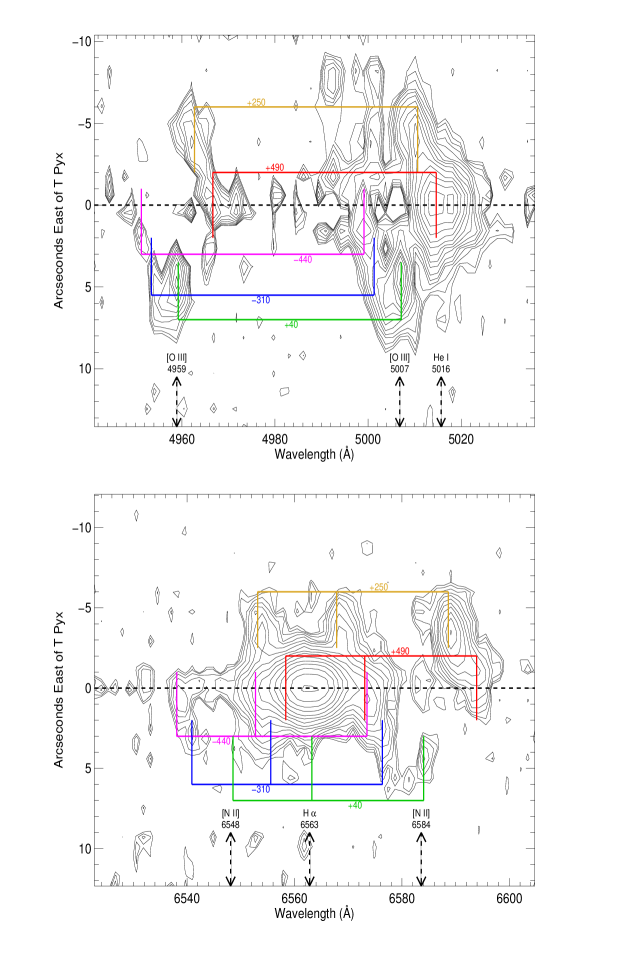
Figure 2: Intensity contours of spatially-resolved, continuum-subtracted spectra of T Pyx and the surrounding region. These data are identical to those of Figure 1, but in addition include the region $\pm 10^{\prime\prime}$ East and West of the star. Each contour is $2\times$ the intensity of the previous one. Each colored bar identifies a system of nebular gas at one consistent velocity, calculated from the detection of two or more emissions lines from the group of [N II] $\lambda\lambda$6548, 6584, H$\alpha$, and [O III] $\lambda\lambda$ 4959, 5007; the reddest colors have the largest recessional velocities, and the bluest, the largest approach. The absolute, heliocentric-corrected velocity values suggested for each system may have uncertainties as large as $\pm 10$ km s^-1, but relative velocities should be substantially more accurate. For reference, the broken lines show the rest wavelengths of these emission features, as well as that of the He I $\lambda 5016$ line, which is detected strongly in the stellar spectrum. We suggest that the prominent, anomalous $\lambda 6590$ emission line (Figure 1) is formed by the superposition of red-shifted [N II] $\lambda 6584$ from the red and orange systems, seen very clearly in this Figure.

References

- (1) Duerbeck, H. W., & Seitter, W. C. 1979, ESO Mess., 17, 1
- (2) Duerbeck, H. W., & Seitter, W. C. 1987, Ap&SS, 131, 467
- (3) Filippenko, A. V. 1982, PASP, 94, 715
- (4) Leavitt, H. 1914, Astr. Nach., 197, 407
- (5) Livio, M. 1998, in Proc. 13th North American Workshop on Cataclysmic Variables, ed. S. Howell, E. Kuulkers, & C. Woodward (San Francisco: ASP), in press
- (6) Massey, P., & Gronwall, C. 1990, ApJ, 358, 344
- (7) Massey, P., Strobel, K., Barnes, J. V., & Anderson, E. 1988, ApJ, 328, 315
- (8) Shahbaz, T., Livio, M., Southwell, K. A., & Charles, P. A. 1997, ApJ, 484, L59
- (9) Shara, M. M., Moffat, A. F. J., Williams, R. E., & Cohen, J. G. 1989, ApJ, 337, 720
- (10) Shara, M. M., Zurek, D. R., Williams, R. E., Prialnik, D., Gilmozzi, R., & Moffat, A. F. J. 1997, AJ, 114, 258
- (11) Webbink, R. F., Livio, M., Truran, J. W., & Orio, M. 1987, ApJ, 314, 653
- (12) Williams, G. 1983, ApJS, 53, 523
- (13) Williams, R. E. 1982, ApJ, 261, 170
- (14) Williams, R. E. 1989, AJ, 97, 1752