Properties of discontinuous and nova–amplified mass transfer in CVs

Abstract

We investigate the effects of discontinuous mass loss in recurrent outburst events on the long–term evolution of cataclysmic variables (CVs). Similarly we consider the effects of frictional angular momentum loss (FAML), i.e. interaction of the expanding nova envelope with the secondary. The Bondi–Hoyle accretion model is used to parameterize FAML in terms of the expansion velocity $v_{\rm exp}$ of the nova envelope at the location of the secondary; we find that small $v_{\rm exp}$ causes strong FAML.

Numerical calculations of CV evolution over a wide range of parameters demonstrate the equivalence of a discontinuous sequence of nova cycles and the corresponding mean evolution (replacing envelope ejection by a continuous wind), even close to mass transfer instability. A formal stability analysis of discontinuous mass transfer confirms this, independent of details of the FAML model.

FAML is a consequential angular momentum loss which amplifies the mass transfer rate driven by systemic angular momentum losses such as magnetic braking. We show that for a given $v_{\rm exp}$ and white dwarf mass the amplification increases with secondary mass and is significant only close to the largest secondary mass consistent with mass transfer stability. The amplification factor is independent of the envelope mass ejected during the outburst, whereas the mass transfer amplitude induced by individual nova outbursts is proportional to it.

In sequences calculated with nova model parameters taken from Prialnik & Kovetz [1995] FAML amplification is negligible, but the outburst amplitude in systems below the period gap with a white dwarf mass $\simeq 0.6M_{\odot}$ is larger than a factor of 10. The mass transfer rate in such systems is smaller than $10^{-11}M_{\odot}$/yr for $\simeq 0.5$ Myr ($\simeq 10\%$ of the nova cycle) after the outburst. This offers an explanation for intrinsically unusually faint CVs below the period gap.

1 Introduction

Cataclysmic variables (CVs) are short–period binary systems in which a Roche–lobe filling low–mass main–sequence secondary transfers mass to a white dwarf (WD) primary. The transferred matter accretes onto the WD either through a disc or a stream and slowly builds up a hydrogen–rich surface layer on the WD. With continuing accretion the pressure at the bottom of this layer increases, and hydrogen burning eventually starts. The thermodynamic conditions at ignition determine how the burning proceeds (e.g. Fujimoto 1982). If the degeneracy is very high, a thermonuclear runaway occurs, leading to a violent outburst terminated by the ejection of all or most of the accumulated envelope. Classical novae are thought to be objects undergoing such an outburst (cf. Livio 1994 for a recent review). Ignition at moderate or weak degeneracy causes strong or weak H shell flashes, whereas stable or stationary hydrogen burning requires fairly high accretion rates $\ga 10^{-7}M_{\odot}/$yr which are not expected to occur in CVs.

Mass transfer in CVs is driven by orbital angular momentum losses which generally shrink the binary and maintain the semi–detached state. The observed properties of short–period CVs below the CV period gap (orbital period $P\la 2$ h) are consistent with gravitational wave radiation as the only driving mechanism. A much stronger angular momentum loss, usually assumed to be magnetic stellar wind braking, is needed for systems above the gap ($P\ga 3$ h). The assumption that magnetic braking ceases to be effective once the secondary becomes fully convective in turn provides a natural explanation for the period gap as a period regime where the systems are detached and therefore unobservable (Spruit & Ritter 1983, Rappaport et al. 1983). The resulting typical mass transfer rate $X$ in CVs is $X\simeq 5\times 10^{-11}M_{\odot}/$yr below the gap and $X\simeq 10^{-9}-10^{-8}M_{\odot}/$yr above the gap (see e.g. King 1988, Kolb 1996, for reviews).

For negligible wind losses from the system the accretion rate is essentially the same as the transfer rate. With the above typical values the H ignition on the WD turns out to be degenerate enough to cause more or less violent outbursts (e.g. Prialnik & Kovetz 1995). As the mass to be accumulated before ignition is very small ($\Delta M_{\rm ig}\simeq 10^{-6}-10^{-3}M_{\odot}$) the outbursts recur on a time $t_{\rm rec}=\Delta M_{\rm ig}/X$ much shorter than the mass transfer timescale which determines the long–term evolution. Studies of the secular evolution of CVs make use of this fact and replace a sequence of nova outbursts with given recurrence time $t_{\rm rec}$ and ejected envelope mass $\Delta M_{\rm ej}$ by a continuous isotropic wind loss from the WD at a constant rate $\Delta M_{\rm ej}/t_{\rm rec}$.

Such a procedure obviously neglects any effect that nova outbursts may have on the long–term evolution. These are in particular
(i) The evolution of the system is not continuous but characterized by sudden changes of the orbital parameters, causing the mass transfer rate to fluctuate around the continuous wind average value (see Sect. 2). It is not a priori clear if the continuous wind average properly describes the system’s evolution close to mass transfer instability.
(ii) At visual maximum (and the following decline) nova envelopes have pseudo–photospheric radii of typical giants, i.e. much larger than the orbital separation. Therefore the secondary is engulfed in this envelope and possibly interacting with it. Drag forces on the secondary moving within the envelope can lead to frictional angular momentum loss (FAML) from the orbit, and accretion of envelope material onto the secondary could increase its photospheric metal abundances (pollution).
(iii) The H burning hot WD is extremely luminous ($\sim 10^{\rm 4}L_{\odot}$, compared with accretion luminosities $\sim 1L_{\odot}$) for as long as a few years. This might drive additional mass loss from the secondary star.

In this paper we will focus on the effects of mass loss discontinuities and FAML. We neglect irradiation as it does not last long enough to influence the long–term evolution. Pollution is expected to be important only for metal poor secondaries (Stehle 1993); we neglect it altogether.

In Sect. 2 we formally derive the continuous wind average and consider the stability of mass transfer in the presence of nova discontinuities analytically, with FAML of arbitrary strength. We review previous studies on FAML and follow Livio et al. [1991] to derive a simple quantitative model for FAML in Sect. 3. Using this description we perform numerical calculations of the long–term evolution of CVs with various strengths of FAML, both for sequences of nova outbursts and the continuous wind average. Results of such computations where the FAML strength and the ejected mass per outburst have been varied systematically are shown in Sect. 4. Sequences with FAML parameters taken from the consistent set of nova models by Prialnik & Kovetz [1995] are shown at the end of Sect. 4. Section 5 discusses our results.

2 Mass transfer stability and classical novae

We begin by investigating how mass transfer discontinuities induced by nova outbursts affect mass transfer stability. Introducting the well–known conservative mass transfer stability criterion we develop a formalism to extend its applicability to the discontinuous case. The strength of FAML enters as a free parameter.

2.1 Conservative and continuous CV evolution

Following Ritter [1988] the mass transfer rate $X$ in a CV can be approximated by

$$X\equiv-\dot{M}_{\rm 2}=\dot{M}_{\rm 0}\;\exp\left(\frac{R_{\rm 2}-R_{\rm R}}{H_{\rm p}}\right)\,,$$ (1)

(note that $X$ is always positive). Here both $\dot{M}_{\rm 0}$ $\simeq$ $10^{\rm-8}M_{\odot}\>{\rm yr}^{\rm-1}$ and the ratio $\epsilon=H_{\rm p}/R_{2}\simeq H_{\rm p}/R_{\rm R}\simeq 10^{\rm-4}$ of the photospheric pressure scale height $H_{\rm p}$ to the donor’s radius $R_{2}$ are roughly constant for the secondaries under consideration. The secondary’s Roche radius $R_{\rm R}$ can be written as a fraction $f_{2}$ of the orbital distance $a$,

$$R_{\rm R}=f_{\rm 2}(q)\>a\,.$$ (2)

$f_{2}$ depends only on the mass ratio $q=M_{1}/M_{2}$ and is for $q>1.25$ given by $f_{2}(q)\simeq(8/81(1+q))^{1/3}$ to better than $2\%$ (Paczyński 1971).

To assess how $X$ changes with time and to find a stationary value for $X$ (where $\dot{X}=0$) we have to consider both $\dot{R}_{2}$ and $\dot{R}_{\rm R}$. From the total orbital angular momentum $J$,

$$J=M_{\rm 1}M_{\rm 2}\sqrt{\frac{Ga}{M}}\>,$$ (3)

and the derivative $\beta_{2}={\rm d}\ln f_{2}/{\rm d}\ln q$ ($\simeq-q/3(1+q)$) we find with (2)

$$\frac{\dot{R}_{\rm R}}{R_{\rm R}}=(\beta_{2}-2)\frac{\dot{M}_{1}}{M_{1}}-(\beta_{2}+2)\frac{\dot{M}_{2}}{M_{2}}+\frac{\dot{M}}{M}+2\frac{\dot{J}_{\rm m}+\dot{J}_{\rm sys}}{J}\,,$$ (4)

where $M_{1}$, $M_{2}$ and $M=M_{1}+M_{2}$ denote the primary mass, donor mass and total mass, respectively. In (4) we formally separate “mass–loss related” angular momentum loss $\dot{J}_{\rm m}$, caused by mass which leaves the binary and carries a certain specific angular momentum $j=\nu(J/M)$ (quantified by the dimensionless parameter $\nu$), i.e.

$$\dot{J}_{\rm m}=j\dot{M}=\nu\frac{J}{M}\dot{M}\,,$$ (5)

and “systemic” angular momentum loss $\dot{J}_{\rm sys}$ which operates without (noticeable) mass loss, e.g. gravitational wave radiation and magnetic braking. By combining the mass–changing terms (4) is usually rewritten as

$$\frac{\dot{R}_{\rm R}}{R_{\rm R}}=\zeta_{\rm R}\frac{\dot{M}_{2}}{M_{2}}+2\frac{\dot{J}_{\rm sys}}{J}\>,$$ (6)

thus defining the mass–radius exponent $\zeta_{\rm R}$ of the secondary’s Roche radius. In the simple case of conservative mass transfer where $M=$ constant, i.e. $\dot{M}_{2}=-\dot{M}_{1}$, we find from (4)

$$\zeta_{\rm R}^{c}=2\left(\frac{M_{2}}{M_{1}}-1\right)-\frac{M}{M_{1}}\beta_{2}\>\simeq\>\frac{2}{q}-\frac{5}{3}\>.$$ (7)

In the more general case of an isotropic wind loss at a rate $\dot{M}=(1-\eta)\dot{M}_{2}$, i.e. $\dot{M}_{1}=-\eta\dot{M}_{2}$, we obtain

$$\zeta_{\rm R}=(1-\eta)\frac{2\nu+1}{1+q}+\eta\frac{2}{q}-2-\beta_{2}\left(1+\frac{\eta}{q}\right)\>,$$ (8)

an expression especially useful when $\eta$ and $\nu$ are constant. Figure 1 depicts $\zeta_{\rm R}^{c}$ and $\zeta_{\rm R}$ with $\eta=0$ and either $\nu=1/q$ or $\nu=q$ as a function of $M_{2}$ for $M_{1}=1.2M_{\odot}$.

Similarly, it is standard practice to decompose the secondary’s radius change into the adiabatic response $\zeta_{\rm ad}\dot{M}_{2}/M_{2}$ and the thermal relaxation $K\equiv(\partial\ln R_{2}/\partial t)_{M={\rm const.}}$,

$$\frac{\dot{R}_{2}}{R_{2}}=\zeta_{\rm ad}\frac{\dot{M}_{2}}{M_{2}}+K\>.$$ (9)

Fig. 2 shows the adiabatic mass–radius exponent $\zeta_{\rm ad}$ as a function of stellar mass for low–mass ZAMS secondaries (Hjellming 1989). Fully convective stars and stars with deep convective envelopes ($M_{2}\la 0.5M_{\odot}$) have $\zeta_{\rm ad}\simeq-1/3$.

Figure 1: Reaction of the secondary’s Roche radius to mass transfer and mass loss, as a function of $M_{2}$ for fixed $M_{\rm 1}=1.2\>M_{\rm\odot}$. Plotted is the mass–radius exponent for conservative mass transfer ($\zeta_{\rm R}^{c}$; full line), isotropic wind with $\eta=0$, $\nu=1/q$ ($\zeta_{\rm R}$ from (8); long dashed), and isotropic wind with $\eta=0$, $\nu=q$ (short dashed). Also shown is $\zeta_{\rm R}^{F}$ for various values of $K_{1}$ (see Sect. 3.1).

Figure 2: Reaction of the secondary’s radius to mass loss as a function of stellar mass $M_{2}$. Full line: adiabatic mass–radius index $\zeta_{\rm ad}$; dotted line: thermal mass–radius index $\zeta_{\rm e}$.

Using these definitions the time derivative of $X$ according to (1) becomes

$$\dot{X}=X\>\left[{\cal A}-{\cal B}X\right]\>,$$ (10)

with

$${\cal A}=\frac{1}{\epsilon}\>\left(K-2\frac{\dot{J}_{\rm sys}}{J}\right)$$ (11)

and

$${\cal B}=\frac{1}{\epsilon M_{2}}\>\left(\zeta_{\rm ad}-\zeta_{\rm R}\right)\>.$$ (12)

The binary attempts to settle at the stationary mass transfer rate

$$X_{s}=\frac{\cal A}{\cal B}=M_{2}\>\frac{K-2\dot{J}_{\rm sys}/J}{\zeta_{\rm ad}-\zeta_{\rm R}}$$ (13)

($\dot{X}=0$ for $X=X_{s}$). The stationary rate is stable if $\partial\dot{X}/\partial X<0$ at $X=X_{s}$, i.e. if the system opposes any instantaneous perturbation in $X$. This translates into ${\cal B}>0$, hence the familiar criterion

$$\zeta_{\rm ad}-\zeta_{\rm R}>0\Leftrightarrow\mbox{mass transfer (dynamically) stable}\>.$$ (14)

A similar stability criterion, $\zeta_{\rm e}-\zeta_{\rm R}>0$, against thermal timescale mass transfer can be derived (see e.g. Ritter 1996), where $\zeta_{\rm e}$ is the thermal equilibrium mass–radius exponent ($\simeq 0.85$ for low–mass main–sequence stars, see Fig. 2).

2.2 Non–stationary mass transfer

The differential equation (10) governs the evolution of the mass transfer rate as a function of time $t$. For constant $\cal A$ and $\cal B$ the solution of (10) is

$$\frac{1}{X(t)}=\frac{1}{X_{s}}-\left(\frac{1}{X_{s}}-\frac{1}{X_{0}}\right)\exp\left(-{\cal A}t\right)\>,$$ (15)

where $X_{0}\equiv X(t=0)$ denotes the initial value of $X$. Hence any changes of the transfer rate proceed on the characteristic timescale $t_{c}=1/{\cal A}\sim{\cal O}(\epsilon t_{J})$, i.e. $t_{c}$ is a small fraction $\epsilon$ of the systemic angular momentum loss timescale $t_{J}=-J/\dot{J}_{\rm sys}$.

In reality both $\cal A$ and $\cal B$ change with time, typically on a the secular timescale $t_{J}$, but for most practical cases where we investigate mass transfer stability against short timescale perturbations $\cal A$ and $\cal B$ can be considered as constant.

Formally (15) is a solution of (10) even if ${\cal A}<0$ (i.e. $\left|K\right|>\left|2\dot{J}_{\rm sys}/J\right|$). In this case, assuming dynamical stability (${\cal B}>0$), $X_{s}$ is negative and no longer a stationary value for the mass transfer rate. Rather (15) shows that in this case $X$ decreases exponentially, i.e. the system detaches (note that $X_{0}$ is a physical mass transfer rate and as such always positive). If finally the mass transfer is unstable (${\cal B}<0$) then we see from (10) that unless $\cal A$ has a large negative value the transfer rate grows. The growth timescale is initially $t_{c}$, but becomes shorter and shorter with further increasing $X$.

2.3 Nova–induced discontinuities

So far we considered only continuous (though not necessarily stationary) mass transfer. Events that change orbital parameters on a timescale much shorter than the characteristic time $\epsilon t_{J}\simeq 10^{4}$ yr for reestablishing the local stationary value $X_{s}$ may be regarded as discontinuous and instantaneous. Nova outbursts certainly belong to this category; the nova envelope expands beyond the orbit within less than a few $10^{2}$ days after ignition and returns within $1-10$ years (actually these are upper limits for the slowest novae). In the following we apply the above formalism separately to the outburst phase and the inter–outburst phase, then combine them to describe the full nova cycle.

2.3.1 Outburst phase

As a result of the outburst the envelope mass $\Delta M_{\rm ej}$ is ejected. We expect that the specific angular momentum carried away by $\Delta M_{\rm ej}$ is higher than the specific orbital angular momentum of the WD due to dynamical friction of the secondary orbiting within the envelope (FAML). Hence we write for the discontinuous change of the orbital angular momentum

$$\Delta J=-(\nu_{1}+\nu_{\rm FAML})\frac{J}{M}\Delta M_{\rm ej}\,,$$ (16)

where $\nu_{1}=M_{2}/M_{1}$ accounts for the specific orbital angular momentum $j=j_{1}$ of the WD (represented as a point mass). The free parameter $\nu_{\rm FAML}$ measures the strength of FAML and will be estimated in terms of a simple model for the frictional processes in Sect. 3 below.

Correspondingly, using (4) with $\Delta M=\Delta M_{1}=-\Delta M_{\rm ej}$ and $\Delta M_{2}=0$ (i.e. neglecting the small amount of mass accreted onto the secondary as well as any mass transfer during this short phase), the change $\Delta R_{\rm R}=R_{\rm R}(\mbox{post})-R_{\rm R}(\mbox{pre})$ of the Roche radius is

$${\left(\frac{\Delta R_{\rm R}}{R_{\rm R}}\right)}_{\rm out}=\frac{\Delta M_{\rm ej}}{M_{1}}\left(\frac{q}{1+q}-\beta_{2}-\frac{2q}{1+q}\nu_{\rm FAML}\right)\,.$$ (17)

2.3.2 Inter–outburst phase

After the outburst mass transfer continues. Once the mass accreted onto the WD exceeds the critical ignition mass $\Delta M_{\rm ig}>0$ the next outburst occurs. For simplicity we assume conservative mass transfer during the inter–outburst phase. According to (6) the total change of the Roche radius in the inter–outburst phase is

$${\left(\frac{\Delta R_{\rm R}}{R_{\rm R}}\right)}_{\rm inter}=\zeta_{\rm R}^{c}\frac{-\Delta M_{\rm ig}}{M_{2}}+2\frac{\Delta J_{\rm sys}}{J}\>,$$ (18)

where $\Delta J_{\rm sys}$ is the total change of the orbital a.m. due to systemic losses between outbursts.

2.3.3 Combined description

For the study of the long–term evolution of CVs it is convenient to replace the sequence of nova cycles with mass transfer discontinuities by a mean evolution where the mass $\Delta M_{\rm ej}$ is regarded as being lost continuously at a constant rate over the cycle in form of an isotropic stellar wind carrying the specific orbital angular momentum $\left(\nu_{1}+\nu_{\rm FAML}\right)J/M$. If $\zeta_{\rm R}^{F}$ denotes the corresponding Roche lobe index then we have from (6)

$${\left(\frac{\Delta R_{\rm R}}{R_{\rm R}}\right)}_{\rm total}=\zeta_{\rm R}^{F}\frac{\Delta M_{2}}{M_{2}}+2\frac{\Delta J_{\rm sys}}{J}\>,$$ (19)

again with $\Delta M_{2}=-\Delta M_{\rm ig}$ because we neglect any change of $M_{2}$ during outburst. As the total change of the Roche radius over a complete cycle is $\Delta R_{\rm R}(\mbox{total})=\Delta R_{\rm R}(\mbox{out})+\Delta R_{\rm R}(\mbox{inter})$, comparison with (17) and (18) gives

$$\zeta_{\rm R}^{F}=\zeta_{\rm R}^{c}+\frac{{\left(\Delta R_{\rm R}/R_{\rm R}\right)}_{\rm out}}{-\Delta M_{\rm ig}/M_{2}}\>.$$ (20)

This can be written as

$$\zeta_{\rm R}^{F} = \zeta_{\rm R}^{c}-\frac{1-\eta^{n}}{q}\left(\frac{q}{1+q}-\beta_{2}-\frac{2\>q}{1+q}\nu_{\rm FAML}\right)$$

$$\simeq \zeta_{\rm R}^{c}-\frac{1-\eta^{n}}{1+q}\left(\frac{4}{3}-2\>\nu_{\rm FAML}\right)\>.$$

Here $1-\eta^{n}=\Delta M_{1}/\Delta M_{2}=\Delta M_{\rm ej}/\Delta M_{\rm ig}$ specifies the change of the WD mass during outburst in units of the mass lost from $M_{2}$ during the inter–outburst phase. Equation (2.3.3) in fact is equivalent to (8) with $\eta=\eta^{n}$ and $\nu=\nu_{1}+\nu_{\rm FAML}$; $\eta^{n}$ determines if the WD mass will grow or shrink in the long–term evolution.

The generalization of (2.3.3) which allows for non–conservative mass transfer between outbursts and a change of $M_{2}$ during outburst is given in the Appendix.

2.4 Stability of discontinuous mass transfer

As was shown in Sect. 2.1 mass transfer in the fictious mean evolution which mimics the effect of nova outbursts by a continuous wind loss is dynamically stable if

$$\zeta_{\rm ad}-\zeta_{\rm R}^{F}>0\>.$$ (22)

Clearly, in the case of discontinuous mass transfer with nova cycles the stability considerations leading to this criterion are no longer applicable, as the system never settles at a stationary transfer rate. After an outburst the transfer rate $X$ follows the solution (15) and approaches the conservative stationary rate $X_{s}^{c}={\cal A}/{\cal B}^{c}$ (where ${\cal B}^{c}$ is ${\cal B}$ according to (12) with $\zeta_{\rm R}^{c}$). At the next outburst $X$ changes discontinuously from the pre–outburst value $X_{\rm pre}$ to the (new) post–outburst value $X_{\rm post}$, i.e. increases (or drops) by a factor

$$\frac{X_{\rm post}}{X_{\rm pre}}=\exp\left[-\frac{1}{\epsilon}\left(\frac{\Delta R_{\rm R}}{R_{\rm R}}\right)_{\rm out}\right]\>,$$ (23)

see Eqs. (1) and (17). In the following we consider mass transfer stability in the presence of nova cycles and derive a generalized stability criterion that reduces indeed to the simple form (22).

In our approach we compare the mass transfer rate $X_{\rm pre}^{i}$ and $X_{\rm pre}^{i+1}$ immediately before subsequent outbursts $i$ and $i+1$ in a sequence of cycles with constant $\Delta M_{\rm ig}$, $\Delta M_{\rm ej}$, ${\cal B}^{c}$ and $\cal A$. Eq. (15) with $X_{0}=X^{i}_{\rm post}$ describes $X$ as a function of time between outbursts. At time $t=t_{\rm rec}$ when the outburst $i+1$ ignites, the mass transferred since the last outburst is just $\Delta M_{\rm ig}$, i.e.

$$\int_{\rm 0}^{t_{\rm rec}}X(t)\>{\rm d}t=\Delta M_{\rm ig}\>.$$ (24)

This can be solved for the outburst recurrence time $t_{\rm rec}$ (cycle time)

$$t_{\rm rec}=\frac{1}{{\cal A}}\>\ln\left[1+\frac{\exp\left({\cal B}^{c}\>\Delta M_{\rm ig}\right)-1}{X^{i}_{\rm post}/X_{s}^{c}}\right]\>.$$ (25)

Inserting $t_{\rm rec}$ for $t$ in (15) gives the new pre–outburst value $X^{i+1}_{\rm pre}=X(t_{\rm rec})$,

$$X^{i+1}_{\rm pre}=X_{s}^{c}\left[1-\exp(-{\cal B}^{c}\Delta M_{\rm ig})\right]$$ (26)

$$+X^{i}_{\rm pre}\exp\left(-{\cal B}^{F}\Delta M_{\rm ig}\right)\>,$$

where we used (23) to replace $X^{i}_{\rm post}$ by $X^{i}_{\rm pre}$, (20) and the definition of ${\cal B}^{F}$ analogous to ${\cal B}^{c}$, i.e. ${\cal B}^{F}=(\zeta_{\rm ad}-\zeta_{\rm R}^{F})/\epsilon M_{2}$. Hence the relative change of the pre–outburst value is

$${\cal F}\hbox to0.0pt{$\displaystyle(X^{i})=\frac{X^{i+1}-X^{i}}{X^{i}}=$\hss}$$ (27)

$$\frac{X_{s}^{c}}{X^{i}}\left[1-\exp(-{\cal B}^{c}\Delta M_{\rm ig})\right]-\left[1-\exp\left(-{\cal B}^{F}\Delta M_{\rm ig}\right)\right]$$

$$\simeq\Delta M_{\rm ig}\left(\frac{{\cal A}}{X^{i}}-{\cal B}^{F}\right)$$

(the subscripts for all $X$ have been dropped as they all read “pre”). We will refer to $\cal F$ as the growth function.

For ${\cal F}>0$ the mass transfer rate grows from outburst to outburst, for ${\cal F}<0$ it decreases, on a timescale $t_{\rm rec}/{\cal F}$. Formally, ${\cal F}=0$ for $X=\tilde{X}$, with

$$\tilde{X}=X_{s}^{c}\frac{1-\exp\left(-{\cal B}^{c}\Delta M_{\rm ig}\right)}{1-\exp\left(-{\cal B}^{F}\Delta M_{\rm ig}\right)}\simeq\frac{\cal A}{{\cal B}^{F}}\>.$$ (28)

$\tilde{X}$ represents the stationary pre–outburst mass transfer rate if it is positive, i.e. if $\cal A$ and ${\cal B}^{F}$ have the same sign. For it to be stable we require $\partial{\cal F}/\partial X^{i}<0$ at $X^{i}=\tilde{X}$ so that the system evolves back to $\tilde{X}$ after a perturbation increases/decreases $X$. This is the case if, and only if, ${\cal A}>0$. Then the stationary solution exists only if ${\cal B}^{F}>0$, in all other cases the system either detaches, or the transfer rate grows unlimited. Figure 3 summarizes schematically the formal functional dependency of $\cal F$ on $X^{i}$ for various combinations of the signs of $\cal A$ and ${\cal B}^{F}$ (see Table 1). Hence the generalized stability criterion for discontinuous nova–amplified mass transfer is ${\cal B}^{F}>0$, which is indeed equivalent to (22). Remarkably, this condition is independent of the sign of ${\cal B}^{c}$, i.e. the system can evolve in a stable manner with formally dynamically unstable conservative mass transfer between subsequent outbursts.

Figure 3: Growth function ${\cal F}$, defined in Eq. (27), as a function of pre–outburst mass transfer rate $X^{i}$ (schematically). See Table 1 for a description of the different curves. Only the solid curve represents a stable stationary solution $\tilde{X}$ (marked by a filled diamond), all other cases lead to a runaway or a turn–off.

Table 1: Branches of possible solutions of Eq. (27) as shown in Fig. 3.

line	sign of		stationary
style	${\cal A}$	${\cal B}^{F}$	solution
full	+	+	yes (stable)
long dashes	–	–	yes (unstable)
dotted	+	–	no
short dashes	–	+	no

The analysis of the system’s behaviour once it violates condition (22) is not straightforward. The main problem is that $\cal A$ is expected to change its sign (from positive to negative) at about the same time as ${\cal B}^{F}$. This can be seen from an estimate of the thermal relaxation term $K$ if the real evolution is replaced by the continuous wind average: Stehle et al. [1996] have shown that the secular evolution rapidly converges to an attracting evolutionary path characterized by

$$\frac{\dot{R}_{2}}{R_{2}}=\zeta_{\rm e}\frac{\dot{M}_{2}}{M_{2}}\>,$$ (29)

whatever the initial configuration of the system. Assuming stationarity, equating (29) with (6), and (9) with (6) gives after elimination of $\dot{M}_{2}/M_{2}$

$${\cal A}\simeq\frac{-2}{\epsilon}\frac{\dot{J}_{\rm sys}}{J}\frac{\zeta_{\rm ad}-\zeta_{\rm R}^{F}}{\zeta_{\rm e}-\zeta_{\rm R}^{F}}$$ (30)

as an estimate for $\cal A$. Hence ${\cal A}>0$ during a phase of stable, stationary mass transfer, but ${\cal A}<0$ once $\zeta_{\rm ad}<\zeta_{\rm R}^{F}$.

In practice this means that when a stable system, characterized by the full line in Fig. 3, approaches instability, the curve becomes flatter and flatter with $\tilde{X}$ almost constant, and then inverts to the (unstable) long–dashed line.

3 A simple model for FAML

In the previous section we derived analytic expressions describing stationary mass transfer and mass transfer stability in the presence of nova cycles. A non–zero FAML effect was allowed, and the strength of FAML was treated as a free parameter $\nu_{\rm FAML}$. To proceed further and underline the above findings with numerical examples we quantify $\nu_{\rm FAML}$ by adopting a model for the frictional processes leading to FAML.

MacDonald [1980] discussed for the first time the possibility that an interaction between the secondary and the extended envelope might tap energy from the orbit and thereby reduce the nova decay time. He determined the angular momentum transferred from the orbit to the envelope by describing the nova envelope as a polytrope with index 3 at rest, and restricting the combined nuclear, internal and frictional energy generation to the Eddington luminosity (MacDonald 1986). Shara et al. [1986] and Livio et al. [1991] used a more direct way, based on Bondi–Hoyle accretion, to estimate the transfer of angular momentum. Their approach (which we adopt below) offers a very simple analytic treatment, as the explicit expression for FAML has only one free parameter, the envelope expansion velocity $v_{\rm exp}$, measuring the strength of FAML. More recently, Kato & Hachisu [1994] have again confirmed their earlier result that FAML has only minor influence on the decay phase of nova outbursts. This can be understood in terms of the high expansion velocities in their models and will be discussed in Sect. 5. On the other hand, Lloyd et al. [1997] showed that common enevlope evolution can contribute to the shaping of the nova remnant.

3.1 FAML description according to Livio et al. [1991]

In Bondi–Hoyle accretion linear momentum is transferred through the drag force

$$\vec{F}_{\rm drag}=-c_{\rm drag}({\cal M},\gamma_{\rm gas})\>\frac{1}{2}\>\pi\>R_{\rm A}^{\rm 2}\>\rho\>v_{\rm rel}\vec{v}_{\rm rel}\>,$$ (31)

where $\vec{v}_{\rm rel}$ is the gas stream velocity at infinity, $R_{\rm A}$ the accretion radius (see below) and $\rho$ the density of the accreted medium. The dimensionless drag coefficient $c_{\rm drag}$ varies with Mach number $\cal M$ and specific heat ratio $\gamma_{\rm gas}$ and is of order unity. Equation (31) is strictly valid for the highly supersonic case, but also applicable for ${\cal M}\ga 1$ if an adequate interpolation for the accretion radius is used, e.g.

$$R_{\rm A}=\frac{2\>G\>M_{\rm 2}}{v_{\rm rel}^{\rm 2}+c_{\rm S}^{\rm 2}}$$ (32)

(Shima et al. 1985); $c_{\rm S}$ is the local sound speed. Detailed 3–dim. hydrodynamical calculations summarized in Ruffert [1995] confirm that (31) describes the subsonic case as well when $\pi R_{\rm A}^{2}$ is replaced by the geometrical cross–section. But these simulations also reveal additional complexities not represented in the simple form (31), e.g. the influence of the accretor’s size, even in the supersonic case. Most important, the drag coefficient can deviate significantly from unity. Kley et al. [1995] point out that radiation pressure may reduce $c_{\rm drag}$ by a factor of $\sim 20$ because it increases the sound speed and thus lowers $\cal M$ to the subsonic case.

Given these uncertainties, and the fact that idealized Bondi–Hoyle accretion is merely a rough approximation to the situation of a secondary orbiting in an expanding nova envelope, the quantitative expressions for FAML derived below are order of magnitude estimates only.

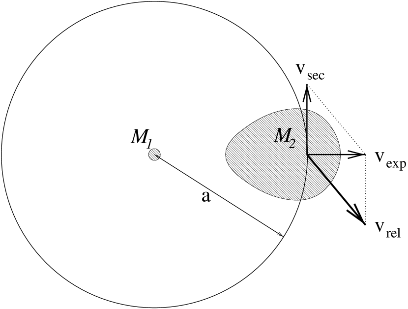
Figure 4: Sketch of the simplified geometry assumed to derive $\nu_{\rm FAML}$. The WD ($M_{\rm 1}$) is at rest and orbited by the secondary ($M_{\rm 2}$) at distance $a$ with velocity $v_{\rm sec}$. The envelope expands spherically symmetric from the WD, and has constant expansion velocity $v_{\rm exp}$ at the location of the secondary.

We now consider the FAML situation in a simplified geometry (Fig. 4): the WD is at rest in the centre of a spherically symmetrical expanding nova envelope. Then the secondary’s orbital velocity

$$v_{\rm sec}=\sqrt{\frac{G\left(M_{\rm 1}+M_{\rm 2}\right)}{a}}$$ (33)

(typically $v_{\rm sec}\simeq 400-500$ km/s) is perpendicular to the wind expanding with $v_{\rm exp}$. Hence the velocity of the accretion flow with respect to the secondary is

$$v_{\rm rel}=\sqrt{v_{\rm sec}^{\rm 2}+v_{\rm exp}^{\rm 2}}.$$ (34)

As $M_{2}/M_{\odot}\simeq R_{2}/R_{\odot}$ the ratio of accretion radius (32) to stellar radius $R_{2}$ is

$$\frac{R_{\rm A}}{R_{2}}\simeq\left(\frac{360{\rm km/s}}{v}\right)^{2}$$ (35)

(where $v$ is the quadratic mean of $v_{\rm sec}$, $v_{\rm exp}$ and $c_{\rm S}$), suggesting that $R_{\rm A}<R_{2}$ for most cases.

Setting $c_{\rm drag}=2$ and $R_{\rm A}=R_{2}$ we obtain for the loss of angular momentum due to friction from the tangential component of the drag force (31)

$$\dot{J}_{\rm FAML}=-|\vec{a}\times\vec{F}_{\rm drag}|=-a\>\pi\>R_{\rm 2}^{\rm 2}\>\rho\>v_{\rm sec}\>v_{\rm rel}.$$ (36)

Using the continuity equation

$$-\dot{M}_{\rm 1}=4\pi\>r^{\rm 2}\rho\>v_{\rm exp}$$ (37)

to eliminate $\rho$, (33) and (2) then give

$$\dot{J}_{\rm FAML}=\frac{1}{4}\>\left[f_{\rm 2}(q)\right]^{\rm 2}\>\frac{v_{\rm rel}}{v_{\rm exp}}\>\dot{M}_{\rm 1}\>\sqrt{G\>M\>a}.$$ (38)

If most of the mass and angular momentum can be assumed to be lost at roughly constant rate and velocity (Livio et al. 1991) we finally obtain the total FAML, integrated over the outburst,

$$\Delta J_{\rm FAML}=-J\>\frac{\Delta M_{\rm ej}}{M_{\rm 1}}\>A(q)\>B(K_{\rm 1}),$$ (39)

where

$$A(q)=\frac{1+q}{4}\left[f_{\rm 2}(q)\right]^{\rm 2},$$ (40)

$$B(K_{\rm 1})=\frac{\sqrt{1+K_{\rm 1}^{\rm 2}}}{K_{\rm 1}}=\frac{v_{\rm rel}}{v_{\rm exp}},$$ (41)

and

$$K_{\rm 1}=\frac{v_{\rm exp}}{v_{\rm sec}}.$$ (42)

Comparison with (16) then shows that

$$\nu_{\rm FAML}=\frac{1+q}{q}A(q)B(K_{\rm 1}),$$ (43)

i.e. the mean specific a.m. $j_{\rm ej}$ of the ejected material is

$$j_{\rm ej}=(\frac{1}{q}+\nu_{\rm FAML})\>\frac{J}{M}.$$ (44)

Figure 5: Top panel: the function $B(K_{1})$ defined in (41). Lower panels: the specific angular momentum $j_{\rm ej}$ of the ejected matter as a function of $K_{1}$ (or $v_{\rm exp}$, obtained by assuming a constant $v_{\rm sec}=400$ km/sec), measuring the strength of FAML, for different mass ratios $q=M_{\rm 1}/M_{\rm 2}$, according to (44). The dashed lines mark the specific a.m. $j_{\rm 1}$ and $j_{\rm 2}$ of the WD and the secondary, respectively.

The functional dependence on $K_{\rm 1}$ in Eq. (41), shown in Fig. 5 (top panel), leads to the unphysical limit $-\Delta J_{\rm FAML}\rightarrow\infty$ for a very slow envelope expansion $v_{\rm exp}\rightarrow 0$. This is mainly due to the neglect of the envelope spin–up which would effectively reduce the relative velocity (Livio et al. 1991).

The secondary cannot spin the envelope up to speeds faster than corotation, so $j_{\rm ej}$ is certainly smaller than $j_{1}+a^{2}\omega$ (where $\omega$ is the binary’s angular velocity). If only a certain fraction of the envelope is spun–up to corotation this upper limit is correspondingly smaller, e.g.

$$j_{\rm max}=j_{1}+(R_{2}/a)a^{2}\omega$$ (45)

if only the torus traced by the secondary’s orbital motion corotates.

Equation (43) specifies our model of FAML in terms of a single parameter, $K_{1}$ (or $v_{\rm exp}$) and determines the value of $\zeta_{\rm R}^{F}$ according to Eq. (2.3.3). We use (45) as a physical upper limit on the effect of FAML.

3.2 The effect of individual nova outbursts

To illustrate the effect of FAML in the parametrization (43) we consider the resulting relative change $\Delta x/x=(x({\rm post})-x({\rm pre}))/x$ of a system parameter $x$ as a result of the nova outburst. For the orbital distance we obtain, similar to (17),

$$\left(\frac{\Delta a}{a}\right)_{\rm out}=\frac{\Delta M_{\rm ej}}{M_{\rm 1}}\left(\frac{q}{1+q}-2\>A(q)\>B(K_{\rm 1})\right)\simeq$$ (46)

$$\quad\quad\quad 10^{-4}\left(1-0.2\>B(K_{\rm 1})\right)\frac{\Delta M_{\rm ej}/10^{-4}M_{\odot}}{m_{1}}\>,$$

which translates into

$$\left(\frac{\Delta P}{P}\right)_{\rm out}=\frac{\Delta M_{\rm ej}}{M_{\rm 1}}\left(2\frac{q}{1+q}-3\>A(q)\>B(K_{\rm 1})\right)\simeq$$ (47)

$$\quad\quad\quad 10^{-4}\left(2-0.6\>B(K_{\rm 1})\right)\frac{\Delta M_{\rm ej}/10^{-4}M_{\odot}}{m_{1}}\>,$$

for the orbital period $P$. The approximate expressions in (46) and (47) make use of the weak dependence on $q$; $m_{1}$ is $M_{1}/M_{\odot}$. For a given ejection mass and white dwarf mass, $B(K_{1})$ critically determines the magnitude of the orbital change. From (23) and (17) the change of the mass transfer rate $X=-\dot{M}_{\rm 2}$ is

$$\left(\frac{\Delta X}{X}\right)_{\rm out}\simeq-\frac{\Delta R_{\rm R}}{H_{\rm p}}=$$ (48)

$$\quad\quad\quad-\frac{\Delta M_{\rm ej}}{M_{\rm 1}}\left(\frac{q}{1+q}-\beta_{\rm 2}(q)-2\>A(q)\>B(K_{\rm 1})\right)\frac{R_{\rm R}}{H_{\rm p}}$$

$$\quad\quad\quad\simeq-\left(1-0.2\>B(K_{\rm 1})\right)\frac{\Delta M_{\rm ej}/10^{-4}M_{\odot}}{m_{1}}\>,$$

where we used $\epsilon\simeq 10^{-4}$ to obtain the last line. Figure 6 illustrates Eq. (48).

Figure 6: Outburst amplitude of the mass transfer rate according to (48) for various strengths of FAML (as labelled) and $\Delta M_{\rm ej}=10^{\rm-4}\>M_{\odot}$, $M_{\rm 1}=1.2\>M_{\odot}$, $H_{\rm p}/R_{\rm R}=1.4\>10^{\rm-4}$.

Depending on the strength of FAML and the mass ratio the changes in system parameters can be either positive or negative. The critical $K_{\rm 1}(q)$ where the amplitudes vanish are shown in Fig. 7. The critical lines for $P$ and $X$ almost coincide and separate the two different outburst types, those which increase the mass transfer rate and decrease the orbital period, and those which decrease the transfer rate and increase the period.

Figure 7: Critical values of $K_{\rm 1}$ where outburst amplitudes resulting from a nova event just vanish, plotted as function of $M_{\rm 2}$ calculated with $M_{\rm 1}=1.2\>M_{\rm\odot}$. Shown are the lines for orbital separation $a$ (full), orbital period $P$ (dotted) and Roche radius $R_{\rm R}$ (dashed, same as for mass transfer rate $-\dot{M}_{\rm 2}$)

3.3 The effect on the long–term continuous wind average

To consider the effect FAML has on the continuous wind average evolution we first note that FAML is a consequential angular momentum loss (CAML; cf. King & Kolb 1995) as $\dot{J}_{\rm FAML}$ is proportional to the mass transfer rate, see (39) with $\Delta M_{\rm ej}=X_{\rm FAML}t_{\rm rec}$ (where $X$ denotes the continuous wind average mass transfer rate). As such FAML amplifies the transfer rate which would be driven by systemic angular momentum losses alone in the absence of FAML.

An analytic estimate of this amplification factor, the ratio $X_{\rm FAML}/X$ of the mass transfer rate with and without FAML, can be obtained if we assume that the system follows the corresponding uniform evolutionary track found by Stehle et al. [1996] also in the case with FAML. This is a reasonable assumption as long as the amplification is moderate and the resulting mass transfer timescale longer than the thermal time of the secondary. The radius reaction of the secondary along its track is given by (29). Hence using $\dot{R}_{\rm R}/R_{\rm R}=\dot{R}_{2}/R_{2}$ and (6) we have

$$\frac{X_{\rm FAML}}{X}\simeq\frac{\left(\zeta_{\rm e}-\zeta_{\rm R}\right)}{\left(\zeta_{\rm e}-\zeta_{\rm R}^{F}\right)}\simeq\left(1-\frac{2\>\frac{1}{q}\>A(q)\>B(K_{\rm 1})}{\zeta_{\rm e}-\zeta_{\rm R}}\right)^{\rm-1}\>.$$ (49)

Here $\zeta_{\rm e}\simeq 0.85\simeq$ const.  and $\zeta_{\rm R}$ is from (8) with $\eta=0$, $\nu=1/q$. We emphasize that the ratio $X_{\rm FAML}/X$ does not depend on the mass $\Delta M_{\rm ej}$ ejected per outburst, rather only on $K_{1}$ and the mass ratio $q$. Fig. 8 shows $X_{\rm FAML}/X$ as function of $1/q$ for various values of $K_{1}$. Obviously FAML amplification is always small for large $q$ (small $M_{2}/M_{1}$). For a given $K_{1}$ it increases with decreasing $q$ and formally goes to infinity where the system approaches thermal instability ($\zeta_{\rm e}=\zeta_{\rm R}^{F}$).

Figure 8: FAML amplification factor $X_{\rm FAML}/X$, defined in (49), as a function of $M_{2}/M_{1}=1/q$, for various values of $K_{1}$. The vertical lines indicate (thermal) instability. The full line is an approximate global upper limit, independent of $K_{1}$.

The full line in Fig. 8 indicates the upper limit for $X_{\rm FAML}/X$ if the specific angular momentum the ejected envelope can carry is limited by $j_{\rm ej}\la j_{1}+(R_{2}/a)a^{2}\omega$ (see Sect. 3.1).

4 Numerical examples

Here we apply the FAML description introduced in the previous section and test the analytical considerations of Sect. 2 and 3 explicitly with numerical sequences of the secular evolution of CVs.

The above FAML model contains $K_{1}$, $\Delta M_{\rm ig}$ and $\Delta M_{\rm ej}$ as free parameters. Unfortunately both observations and theoretical models describing the outburst itself yield often contradicting and inconsistent estimates for these parameters. Therefore we restrict the following investigation to a simple parameter study to obtain a systematic picture of the effect of FAML with a given strength on the secular evolution. In particular we present calculations with constant $\Delta M_{\rm ig}$ ($=\Delta M_{\rm ej}$) and $K_{1}$, for various values of $\Delta M_{\rm ig}$ and $K_{1}$.

4.1 Computational technique

To model the binary evolution numerically we describe the secondary star by either full stellar models using Mazzitelli’s stellar evolution code (e.g. Mazzitelli 1989), or by a simplified bipolytrope structure using the generalized bipolytrope code (Kolb & Ritter 1992). Both codes have been modified to include FAML and to resolve individual nova outbursts.

The bipolytrope code is about 4 orders of magnitude faster than the full code and allows one to compute the secular evolution for several Gyr with every single nova outburst fully resolved. Several sequences calculated with the full code serve as an independent check of the simplified description. Despite a careful calibration of the bipolytrope model to full stellar models, allowing a quantitative match of the results to usually better than 10%, there are well–known limitations of the simplified description (see Kolb & Ritter 1992), e.g. the increasing deviation of $\zeta_{\rm ad}$ from the values of actual stars for $M_{\rm 2}\ga 0.6\>M_{\odot}$. But these effects are negligible for the purpose of this paper.

In all the examples shown below we compute magnetic braking according to Verbunt & Zwaan [1981] with the calibration parameter set to unity.

We have performed calculations with the following two modes:

1. fully resolved: Mass transfer is conservative until the mass accreted on the WD exceeds the ignition mass. In the time step immediately thereafter the ejecta mass and the angular momentum (39) is removed from the system. Thus fully resolved evolutions are discontinuous and show repeating nova cycles.

2. continuous wind average: Mass loss from the system is continuous at a rate equal to the transfer rate, carrying the increased specific angular momentum according to (44); hence the secular evolution is continuous.

4.2 Detailed examples for individual outbursts

Figure 9: Section of a fully resolved evolutionary calculation with nova outbursts after $\Delta M_{\rm ig}=\Delta M_{\rm ej}=10^{\rm-4}M_{\odot}$ with $M_{\rm 1}=1.2\>M_{\odot}$, $M_{\rm 2}\simeq 0.6\>M_{\odot}$ and weak FAML ($K_{\rm 1}=0.5$). Crosses indicate time intervals of 1000 years, the filled diamond the post–outburst model from which initial values for the analytical approximation (dotted line) were taken. The additional horizontal lines are explained in the text.

Figure 10: As Fig.9, but with strong FAML ($K_{\rm 1}=0.1$).

We generated short stretches of fully–resolved evolutionary sequences with full stellar models by switching into the fully resolved mode in the middle of a continuous wind average calculation for a typical CV above the period gap. The mode switch was made from a model well–established on the uniform evolutionary track characterized by (29).

Fig. 9 shows for the case of weak FAML with $K_{\rm 1}=0.5$ a ’sawtooth’ (or ’shark–fin’) like modulation of the mass transfer rate over the orbital period (full line). The system evolves from right to left; the crosses mark intervals of 1000 yr. As expected from Fig. 7 the outburst results in a longer period and a lower mass transfer rate with this choice of parameters. In the case of strong FAML with $K_{\rm 1}=0.1$ (Fig. 10) the outburst leads to a shorter period and a higher mass transfer rate.

The approximate time evolution according to Eq. (15), with ${\cal A}$ and ${\cal B}^{c}$ evaluated from the full sequence at the post–outburst position, marked with a filled diamond, is shown as a dotted curve and matches the full sequence very well. The dash–dotted line in Figs. 9 & 10 indicates the level of the ’local’ stationary conservative mass transfer rate as given by Eq. (13) with $\zeta_{\rm R}=\zeta_{\rm R}^{c}$. Note that there is a difference between this value and the mass transfer rate of a completely conservative evolution with the same initial values (but no outbursts) as the system here does not evolve conservatively on average but loses mass together with angular momentum. The averaged stationary mass transfer rate which includes FAML with $\zeta_{\rm R}^{F}$ according to Eq. (2.3.3) is shown as a dashed line. This value is identical to the mass transfer rate calculated in the averaged mode and to the time average of the full evolution. The system approaches the conservative value between outbursts and oscillates around the average transfer rate.

Note that if, beginning with negligible FAML, the strength of FAML is continuously increased, the outburst amplitudes will decrease until the stationary (local) conservative transfer rate and the continuous wind average (which grows with FAML) are equal. Further increase of FAML will now lead to growing amplitudes, but with opposite signs.

4.3 Long–term evolution with FAML

Figure 11: Averaged mass transer rate $X$ versus orbital period $P$ for a CV with $M_{\rm 1}=1.2\>M_{\odot}$ and $M_{\rm 2}=1.0\>M_{\odot}$ at turn–on without FAML (full line) and with strong FAML ($K_{\rm 1}=0.1$, corresponding to $v_{\rm exp}\simeq 40$ km/sec; dotted line). Computed with full stellar models.

Fig. 11 compares the continuous wind average evolution for a reference system ($M_{\rm 1}=1.2\>M_{\odot}$; $M_{\rm 2}=1.0\>M_{\odot}$ at turn–on; $\eta=0$) with strong FAML and without FAML, computed with full stellar models. As expected from Fig. 8 the mass transfer rate with FAML is significantly larger than in the case without only at long periods, where the system is close to (but not beyond) thermal instability. Due to the higher mass transfer rate the secondary in the FAML sequence is driven further out of thermal equlibrium and therfore larger at the upper edge of the period gap. At the same time the secondary’s mass is smaller upon entering the detached phase. Both effects, well–known from systematic studies of CV evolution (e.g. Kolb & Ritter 1992), cause a wider period gap by both increasing the period at the upper edge and decreasing the period at the lower edge of the gap.

Figure 12: Set of fully resolved secular evolutions of a CV with $M_{\rm 1}=1.2\>M_{\odot}$ (left) and $M_{\rm 1}=0.65\>M_{\odot}$ (right), computed with the bipolytrope code. From top to bottom the strength of FAML increases as labelled. The evolutionary tracks connect the location immediately before and after an outburst, but not for subsequent outbursts! Rather only every every $1000^{\rm th}$ outburst (thick line, corresponding to $\Delta M_{\rm ig}=5\>10^{\rm-6}M_{\odot}$), or every $100^{\rm th}$ outburst (thin line, corresponding to $\Delta M_{\rm ig}=10^{\rm-4}M_{\odot}$) is shown. The initial secondary mass at turn–on was $M_{\rm 2}=1.0\>M_{\odot}$ for the top three sequences on the left, and $0.4\>M_{\odot}$ on the right. For the sequences in the lowest panel the initial secondary mass was $0.85\>M_{\odot}$ and $0.25\>M_{\odot}$, respectively.

The analytical considerations of Sect. 3.3 are confirmed by a parameter study performed with the bipolytrope code. The evolutionary sequences with all outbursts resolved depicted in Fig. 12 summarize the results. The reference system is shown in the left column, a less massive system in the right column. The strength of FAML increases from top to bottom, with consequences for the outburst amplitudes as discussed in Sect. 3.2 and in the previous subsection. Note that the ’sawtooths’ here do not represent single outburst cycles, but arise because we connect the pre– and post–outburst values for every n^th ($n=1000$ or $100$) outburst only. The advantage of this display method is that both magnitude and sign of the outburst amplitude (the vertical flanks) can be followed through the evolution. In reality the system undergoes many individual cycles like those in Figs. 9 & 10 between subsequent outbursts depicted in Fig. 12. The two evolutionary tracks plotted in each panel differ only in the ignition mass $\Delta M_{\rm ig}$ (here $=\Delta M_{\rm ej}$). The thick line corresponds to $\Delta M_{\rm ig}=5\times 10^{\rm-6}\>M_{\odot}$, the thin line to $\Delta M_{\rm ig}=10^{\rm-4}\>M_{\odot}$. In the scale used the low ignition mass sequences are practically indistinguishable from the continuous wind average evolution (remember that both oscillate around the same average value, cf. Sect. 4.5). Inspection of Fig. 6 shows that the growth of amplitudes towards shortest periods is mainly due to the increase of $q$. Only in the high FAML (low $v_{\rm exp}$) case, i.e. in the very steep region of Eq. (41), there is an additional contribution from the increasing orbital velocity (hence decreasing $K_{\rm 1}$) at short $P$.

4.4 FAML–induced instability

To illustrate and test the analytical mass transfer stability considerations of Sects. 2.3 and 2.4 explicitly we consider the secular evolution of a system which runs into an instability, i.e. violates the formal stability criterion (22) at some point of the evolution.

To establish this situation we artificially increase the strength of FAML along a fully resolved evolutionary sequence (computed with the bipoltrope code, with constant $\Delta M_{\rm ig}=\Delta M_{\rm ej}=10^{-4}M_{\odot}$), starting from a small value at the onset of mass transfer. As a consequence $\zeta_{\rm R}^{F}$ becomes larger than $\zeta_{\rm ad}$ at some intermediate secondary mass. In particular, we adopt

$$\frac{v_{\rm exp}}{{\rm km/s}}=180\frac{M_{2}}{M_{\odot}}-50$$ (50)

as the functional form of the envelope expansion velocity. ($M_{2}$ will be large enough to avoid negative $v_{\rm exp}$). The corresponding $\zeta_{\rm R}^{F}$ with $\nu_{\rm FAML}$ from (43) becomes larger than $\zeta_{\rm ad}$ at $M_{2}\simeq 0.55\>M_{\odot}$, and the mass transfer rate indeed begins to grow without limit at about this mass well above the period gap (Fig. 13). A closer look at the final phase immediately before the runaway (Fig. 14) shows that the system evolves beyond the formally unstable point apparently unaffected and enters the runaway mass transfer phase only $\simeq 10^{6}{\rm yr}$ later. In fact this is just as we would expect if the evolution were replaced by the corresponding continuous wind average. In this case (10) with ${\cal B}={\cal B}^{F}$ describes the variation of the (average) mass transfer rate $X$. The characteristic timescale on which $X$ changes is $X/\dot{X}=1/({\cal A}-{\cal B}^{F}X)$, which becomes very large when ${\cal B}^{F}\simeq 0$, i.e. around $\zeta_{\rm ad}=\zeta_{\rm R}^{F}$ at the instability point; note that ${\cal A}$ is also small at this point, see (30). Proceeding further increases the strength of FAML even more and makes ${\cal B}^{F}$ more negative, hence the timescale $|X/\dot{X}|$ progressively shorter. The time delay until the runaway finally begins is essentially determined by the crossing angle between the functions $\zeta_{\rm ad}(M_{2})$ and $\zeta_{\rm R}^{F}(M_{2})$ and the value of $X$ at this point.

Figure 13: Fully resolved secular evolution of a CV with $M_{\rm 1}=0.8\>M_{\odot}$ and $M_{\rm 2}=0.7\>M_{\odot}$ at turn–on, computed with the bipolytrope code including FAML based on (50) and $\Delta M_{\rm ig}=\Delta M_{\rm ej}=10^{-4}M_{\odot}$. For $\log(P/{\rm h})>0.67$ every $100^{\rm th}$ outburst is shown, for $\log(P/{\rm h})<0.67$ every outburst.

Figure 14: Evolution of the mass transfer rate $X$ with time during the final phase (approximately 2 million years) before the runaway (dotted, filling the grey–shaded area). Overplotted in full linestyle is the stationary value $X_{s}^{F}={\cal A}/{\cal B}^{F}$ for a continuous FAML-increased mass loss, indicating an instability at $\simeq 12.1\>{\rm Myr}$.

Figure 15: Growth function ${\cal F}$ (cf. (28) and Fig. 3) calculated with data taken from the evolution shown in the previous figures for different times as labelled.

Figure 15 shows the growth function ${\cal F}$ defined in (27) for selected models immediately before the runaway for the evolutionary sequence depicted in Fig. 14. The different curves are computed with data from the run taken at the times as labelled (cf. Fig. 14). As discussed in Sect. 2.4 the change of ${\cal F}$ from a stable curve with negative slope to an unstable curve with positive slope occurs when $\zeta_{\rm ad}=\zeta_{\rm R}^{F}$.

The sequence shown in Figs 13-15 is typical of the behaviour of evolutionary sequences with nova cycles and very strong FAML. It convincingly demonstrates that the FAML–amplified istropic wind average properly describes the effect of a sequence of nova outbursts, even in the most extreme case when the system approaches a FAML–induced instability. A more systematic investigation of the significance of this instability for the secular evolution of CVs will be published elsewhere (Kolb et al., in preparation).

4.5 Evolution with FAML parameters from theoretical nova models

The FAML parameters $K_{1}$, $\Delta M_{\rm ej}$ and $\Delta M_{\rm ig}$ are certainly not constant along the evolution but depend on the actual state of the outbursting system. The three governing parameters which crucially determine the outburst characteristics of thermonuclear runaway (TNR) models for classical novae are the WD mass $M_{1}$, the (mean) accretion rate $X$ and the WD temperature $T_{1}$ (e.g. Shara 1989). Both the mass and the temperature of the WD change only slowly during the binary evolution, thus the dominant dependence of $v_{\rm exp}$ is from the (mean) mass transfer rate. As FAML itself drives the mass transfer this could lead to an interesting feedback and possibly self–amplification in the system, a question considered in a separate paper (Kolb et al., in preparation).

Although published TNR models mostly give values for $\Delta M_{\rm ig}$ and estimates for $\Delta M_{\rm ej}$, few or no data are available on $K_{1}$. Unfortunately this is also true for the most complete and consistent set of published nova models (Prialnik & Kovetz 1995) which we chose to use as input to the FAML description derived in Sect. 3.1.

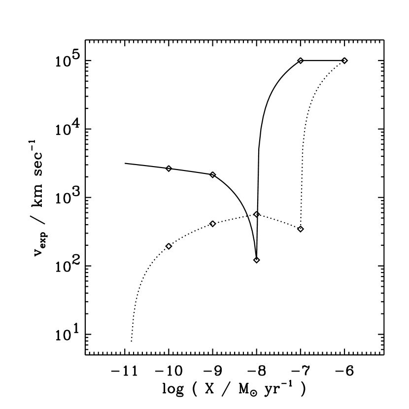
Figure 16: Averaged maximal expansion velocity of the ejecta taken from nova models of Prialnik & Kovetz [1995], with $T_{\rm 1}=10^{\rm 7}$ K and $M_{\rm 1}=0.65\>M_{\odot}$ (full line) or $M_{\rm 1}=1.25\>M_{\odot}$ (dotted line). Diamonds mark real data points. A maximum value of $10^{\rm 5}$ km/sec has been inserted if no ejection occurred to mimic negligible FAML.

These authors tabulate only the average expansion velocity $v_{\rm av}$, the time average of the maximum velocity in the flow during the whole mass loss phase. In the absence of more relevant velocity data we simply set $v_{\rm exp}=v_{\rm av}$, but we are aware that this choice represents an upper limit for $v_{\rm exp}$ (which has to be taken at the secondary’s position). Two exemplary relations $v_{\rm exp}(X)$ are shown in Fig. 16, for a low and a high mass WD, complemented by large values ($10^{5}$ km/sec, hence negligible FAML) when no envelope ejection was found in the hydrodynamical simulations.

Figure 17: Secular evolution of a CV with fully resolved nova cycles and $M_{\rm 1}=1.2\>M_{\odot}$, $M_{\rm 2}=1.0\>M_{\odot}$ at turn–on (thin line), computed with the bipolytrope code. Ignition mass, ejection mass and velocities are taken from Prialnik & Kovetz [1995]. Similar to Fig. 12 only every $100^{\rm th}$ outburst is shown, and straight lines connect post– and pre–outburst points. For comparison the continuous wind average evolution without FAML (thick line) is also shown. At the period minimum the WD mass has decreased to $M_{1}\simeq 1.1\>M_{\odot}$.

Figure 18: As Fig. 17, but with $M_{\rm 1}=0.65\>M_{\odot}$, $M_{\rm 2.i}=0.4\>M_{\odot}$, and every $20^{\rm th}$ outburst shown. At the period minimum the WD mass has decreased to $M_{1}\simeq 0.635\>M_{\odot}$.

The evolutionary sequences obtained with $M_{\rm 1}=1.2\>M_{\odot}$ (using the velocity data for nova models with a $1.25\>M_{\odot}$ WD) and with $M_{\rm 1}=0.65\>M_{\odot}$ are shown in Figs. 17 & 18. The changes of $M_{\rm 1}$ during the whole evolution are very small ($\eta\simeq 0$). As in Fig. 12 the ’sawtooths’ result from connecting only every ${\rm n}^{\rm th}$ outburst. For comparison a standard continuous wind average evolution without FAML but otherwise identical parameters has been overlaid in thick linestyle. As expected from the high expansion velocities FAML has very little effect on the global evolution. By choice we underestimated the strength of FAML in the sequences shown above. But although the expansion velocity at the location of the secondary is indeed smaller than $v_{\rm av}$ in the models by Prialnik & Kovetz [1995] they currently appear to be too large to cause a FAML effect with significance for the long–term evolution of CVs (cf. also discussion in next section).

Perhaps the most interesting feature of the sequences presented in this paragraph is the large outburst amplitude of the mass transfer rate in low–mass WD ($0.65M_{\odot}$) systems below the period gap. The reason for this lies mainly in the fact that $\Delta M_{\rm ej}$ and $\Delta M_{\rm ig}$ to a first approximation scale like $R_{1}^{4}/M_{1}$ (Fujimoto 1982, $R_{1}$ is the WD radius), i.e. increase with decreasing WD mass (and to a lesser extent, increase with decreasing $X$). Moreover the slow but continuous decrease of the WD mass leads to a further increase of the outburst amplitudes towards shorter orbital period in this sequence (Fig. 18). Note that this effect adds to the ones observed before (lowermost panels of Fig. 12) which were caused by the change of $q$ due to decreasing $M_{2}$, and to a lesser extent to the slowly increasing orbital velocity $v_{\rm sec}$, mimicing increasing FAML strength.

Figure 19: A typical inter–outburst low–mass WD CV below the period gap ($M_{1}=0.6382\>M_{\odot}$, $M_{2}\simeq 0.1\>M_{\odot}$, $\Delta M_{\rm ej}=\Delta M_{\rm ig}=2.9\>10^{-4}M_{\odot}$) according to nova parameters from Prialnik & Kovetz [1995]. Shown is the time spent with a mass transfer rate below a value $X$, as a function of $X$ (in $M_{\odot}$/yr). Diamonds indicate the immediate post- or pre–outburst state. The dashed line indicates the continuous wind average mass transfer rate.

Such amplitudes account for a non–negligible time interval with a secular mean mass transfer rate significantly below the continuous wind average transfer rate, i.e. below $\simeq 5\times 10^{-11}M_{\odot}$/yr, the typical value for non–degenerate CVs below the period gap driven by gravitational radiation alone. As an example Fig. 19 plots for a model at $P=1.23$ h from the sequence shown in Fig. 18 the time spent with a mass transfer rate below a value $X$, as a function of $X$. One nova cycle lasts $\simeq 6.5$ Myr, and the mass transfer rate remains for 0.5 Myr after the outburst below $10^{-11}M_{\odot}$/yr. Intrinsically, these CVs with low-mass and moderate–mass WDs form the vast majority (e.g. de Kool 1992, Politano 1996). Thus, ignoring selection effects, we would expect to observe 1 out of 10-20 short–period CVs with small sub–GR driven mass transfer rate.

This seems to offer an alternative explanation for the low mass transfer rate Sproats et al. [1996] claim to find observationally in so–called tremendous outburst amplitude dwarf novae (TOADs) which Howell et al. [1997] interpret as post minimum period systems. As the secular mean mass transfer rate is predicted to drop substantially ($\la 10^{-12}-10^{-11}M_{\odot}$/yr) CVs which have evolved past the minimum period would be even fainter than the above post–outburst CVs, and it is unclear if they are detectable at all.

We note that at least 4 objects in the list of Sproats et al. [1996] have been labelled as novae (cf. Duerbeck 1987): AL Com (orbital period $0.0566$ d, outburst suspected 1961), VY Aqr ($0.0635$ d, 1907), RZ Leo ($0.0708$ d, 1918) and SS LMi (no period known; 1980). With exception of SS LMi they are now firmly considered to be dwarf novae. This does not exclude a priori that the first recorded outburst (e.g. in 1907 for VY Aqr) or even earlier ones were actually novae. Hence it is at least conceivable that the present low mass transfer rate and the TOAD characteristics might be a consequence of this last nova event. The three systems with known orbital period are located at the extreme end of Fig. 4 of Sproats et al. [1996], showing large outburst amplitude and low quiescence magnitude. Moreover, among the open square symbols indicating DNe in their Fig. 3 they are also those with lowest period and absolute magnitude in quiescence (mass transfer rate $\ll 10^{-11}M_{\odot}$/yr). The fact that the claimed deviation from the secular mean magnitude is shrinking with the time elapsed since the potential nova outburst (1961 - 1918 - 1907) is probably just a coincidence.

We caution that it is difficult to decide if the set of models by Prialnik & Kovetz [1995] properly describes classical nova outbursts on WDs in CVs below the period gap. Observationally, only 4 out of 28 classical novae with determined orbital period are below the gap (e.g. Ritter & Kolb 1995). This is in conflict with standard population models of CVs if the Prialnik & Kovetz [1995] ignition masses are used to predict an observable period distribution for novae (Kolb 1995).

5 Discussion and conclusions

In this paper we considered the effects of nova outbursts on the secular evolution of CVs. As a result of these outbursts the secular mean mass transfer rate and the orbital period are not continuous functions of time but change essentially discontinuously with every nova outburst by an amount proportional to the ejected envelope mass. In addition, energy and angular momentum can be removed from the orbit due to dynamical friction of the secondary orbiting in the expanding nova envelope.

The discontinuous evolution with a given strength of frictional angular momentum loss (FAML) is usually replaced by the corresponding continuous wind average evolution, where the mass and angular momentum loss associated with a nova outburst is assumed to be distributed over the inter–outburst time and to form an isotropic wind from the white dwarf. We showed analytically that the well–known mass transfer stability criterion for the latter case can also be derived from a proper analysis of the real, discontinuous process, for an arbitrary strength of FAML–amplification.

We specified a quantitative model for FAML within the framework of Bondi–Hoyle accretion following Livio et al. [1991]. In this model the strength of FAML depends crucially on the expansion velocity $v_{\rm exp}$ of the envelope at the location of the secondary, being the stronger the smaller $v_{\rm exp}$ is. We expect that the resulting simple one–parameter description properly describes the order of magnitude of the FAML effect and, more importantly, the differential dependences on fundamental binary parameters. Hence although it is a useful way to study the potential influence of FAML systematically, it certainly cannot replace a detailed modelling of the frictional processes.

Calculations of the long–term evolution of CVs verified the validity of the replacement of the discontinuous sequence of nova cycles with the continuous wind average, even for situations close to mass transfer instability, whatever the strength of FAML. The mass transfer rate in the continuous wind average evolution is FAML–amplified, i.e. by the factor (49) larger than the transfer rate driven by systemic angular momentum losses alone. For a given CV this factor is determined by $K_{1}$ alone, i.e. independent of the ejection mass. We emphasize that FAML only amplifies the transfer rate caused by systemic losses, it does not add to them. Hence FAML is a particular example of consequential angular momentum losses (CAML) investigated in detail by King & Kolb [1995].

In general, the FAML amplification factor turns out to be large only when the envelope expansion is very slow ($K_{1}\la 0.5$, i.e. $v_{\rm exp}\la 200$ km/s) and when the system is already close to thermal mass transfer instability (Fig.8). This latter condition means that e.g. for an evolution with strong FAML $K_{1}=0.1=$ const. the averaged mass transfer rate is significantly affected only at long orbital period, $P\ga 5$ h.

The magnitude and direction of the outburst amplitudes of the mass transfer rate $X$ and the orbital period $P$ depend on both the ejection mass $\Delta M_{\rm ej}$ and the FAML parameter $K_{1}$. For weak (or negligible) FAML the outbursts are towards lower mass transfer rate and longer orbital period, for strong FAML towards larger $X$ and shorter $P$. There is an intermediate regime where the outburst amplitudes essentially disappear.

Theoretical models for nova outbursts generally find larger expansion velocities (e.g. Prialnik 1986, Prialnik & Kovetz 1995), typically $K_{1}\ga 1$. This is certainly true for the terminal velocities, but in more recent models probably also for the crucial velocity at the secondary’s location, i.e. closer to the WD. Kato & Hachisu [1994] argue that in the wind mass loss phase of a nova outburst the main acceleration (at about the sonic point) takes place at a temperature where the opacity has a maximum. Thus the introduction of the OPAL opacities had the effect of moving this point closer to the WD. A comparison of the radial velocity profiles found by Kato & Hachisu [1994] with those obtained previously (e.g. Prialnik 1986, Kato 1983) confirms this. As a result, in the newer models the velocities at the location of the secondary are already quite close to their terminal values. This explains why Kato & Hachisu [1994] find only marginal effects from dynamical friction.

This seems to suggest that the overall influence of FAML on the long–term evolution of CVs is small. However, in view of the considerable simplifications of our FAML description and the uncertainties of theoretical TNR models for nova outbursts, it is worthwhile to investigate sytematically mass transfer stability with FAML, and to consider the role of a feedback between outburst characteristics (hence FAML strength) and the mean mass transfer rate prior to the outburst. We will study this in a forthcoming paper (Kolb et al., in preparation).

To illustrate further the effect FAML might have on the secular evolution of CVs we have calculated evolutionary sequences with envelope expansion velocities, ignition and ejection masses taken from the extended set of nova models by Prialnik & Kovetz [1995]. As expected, the continuous wind average evolution hardly differs from the standard CV evolution without FAML. As a consequence of the large ejection mass (several $\simeq 10^{-4}M_{\odot}$/yr) the outburst amplitudes become very large (a factor $\ga 10$) below the period gap for intermediate mass WDs ($M_{1}\simeq 0.6M_{\odot}$) — even more so as the outburst–induced decrease of the mass transfer is largest if FAML vanishes.

Such systems have a mass transfer rate less than $10^{-11}M_{\odot}$/yr for $\simeq 0.5$ Myr after the outburst, and could account for intrinsically faint CVs below the period gap. We speculated (Sect. 4.5) if TOADs (e.g. Sproats et al. 1996) could represent such systems.

We finally note that the apparent scatter in observationally derived values for the mass transfer rate of CVs with comparable orbital period, well–known since the review of Patterson [1984], is unlikely to be due to outburst amplitudes. First, we expect from Fig. 17 that these amplitudes are small or negligible above the period gap, and second the systems spend most of the time close to the continuous wind average mass transfer rate (cf. Fig. 19). A more promising explanation for this scatter assumes mass transfer cycles which could be irradiation–induced (e.g. King et al. 1995, 1996).

Acknowledgements.

We thank D. Prialnik and A. Kovetz for giving access to nova model parameters prior to publication, and M. Livio and L. Yungelson for providing a copy of an unpublished manuscript on FAML. K.S. would like to thank M. Ruffert for many discussions on Bondi–Hoyle accretion. We thank A. King for improving the language of the manuscript. K.S. obtained partial financial support from the Swiss National Science Foundation. Theoretical astrophysics research at Leicester is supported by a PPARC rolling grant.

Appendix A Generalization of $\zeta_{\rm R}^{F}$

Starting from the fundamental Eq. (4) one can derive a more general expression for the relative change of $R_{\rm R}$ during both the outburst and inter–outburst phase. Specifically we allow a small fraction $\alpha$ of the mass ejected during the outburst to accrete on to the secondary, i.e. $\Delta M_{2}=\alpha\>\Delta M_{\rm ej}$. This gives

$${\left(\frac{\Delta R_{\rm R}}{R_{\rm R}}\right)}_{\rm out}\hbox to0.0pt{$\displaystyle=\frac{\Delta M_{\rm ej}}{M_{2}}\left[\frac{2-\beta_{2}}{q}-\alpha(\beta_{2}+2)-\right.$\hss}$$ (51)

$$\left.\frac{1-\alpha}{1+q}(1+\frac{2}{q}+2\>\nu_{\rm FAML})\right]$$

instead of (17), which is obtained in the case $\alpha=0$.

Additionally we allow a wind (or other) mass loss during the inter–outburst accretion phase. Thus we use the general $\zeta_{\rm R}$ from (8) rather than the conservative one to generalize (18). This results in two additional parameters, $\eta^{w}$ and $\nu^{w}$, describing the system’s ”wind” mass and corresponding angular momentum loss during the inter–outburst phase. Hence we get (using $\gamma=(\eta^{w}+1)/\eta^{w}$)

$${\left(\frac{\Delta R_{\rm R}}{R_{\rm R}}\right)}_{\rm inter}\hbox to0.0pt{$\displaystyle=2\frac{\Delta J_{\rm sys}}{J}+\frac{\Delta M_{\rm ig}}{M_{2}}\left[\frac{\beta_{2}-2}{q}+\right.$\hss}$$ (52)

$$\left.(\beta_{2}+2)(\gamma-1)-\frac{\gamma-2}{1+q}(1+2\>\nu^{w})\right]\>,$$

which with (51), (19) and $\Delta M_{2}=\alpha\Delta M_{\rm ej}-(\gamma-1)\Delta M_{\rm ig}$ gives the generalized $\zeta_{\rm R}^{F}$

$$\zeta_{\rm R}^{F}=\hbox to0.0pt{$\displaystyle\frac{1}{\Delta M_{2}}\left(\Delta M_{\rm ej}\left[\frac{2-\beta_{2}}{q}-\alpha(\beta_{2}+2)-\right.\right.$\hss}$$ (53)

$$\left.\left.\frac{1-\alpha}{1+q}\left(1+\frac{2}{q}+2\>\nu^{\rm FAML}\right)\right]+\Delta M_{\rm ig}\left[\frac{\beta_{2}-2}{q}+\right.\right.$$

$$\left.\left.(\beta_{2}+2)(\gamma-1)-\frac{\gamma-2}{1+q}(1+2\>\nu^{w})\right]\right)\>.$$

Six parameters describe the system: $\Delta M_{\rm ig}$ and $\Delta M_{\rm ej}$ (ideally taken from nova models), $\nu_{\rm FAML}$ and $\alpha$ (requiring the specification of a particular FAML model), and $\gamma$ (or $\eta^{w}$), $\nu^{w}$ (characterizing the wind loss during accretion).

The ratio of mass retained by the WD to that lost by the secondary

$$\eta=-\left(\frac{\Delta M_{1}}{\Delta M_{2}}\right)_{\rm total}=\frac{\Delta M_{\rm ej}-\Delta M_{\rm ig}}{\alpha\Delta M_{\rm ej}-(\gamma-1)\Delta M_{\rm ig}}\>,$$ (54)

which relates $\Delta M_{\rm ej}$ and $\Delta M_{\rm ig}$ similar to the simple case $\eta^{n}$ in the main body of the paper, now depends on $\alpha$ and $\gamma$. Using a weighted $\nu$ to describe the average specific angular momentum gives

$$\nu=\frac{(\alpha-1)\Delta M_{\rm ej}\left(\frac{1}{q}+\nu_{\rm FAML}\right)-(\gamma-2)\Delta M_{\rm ig}\nu^{w}}{(\alpha-1)\Delta M_{\rm ej}-(\gamma-2)\Delta M_{\rm ig}}\>,$$ (55)

and inserting these values into Eq. (8) would also have directly led to Eq. (53).

References

- [1992] de Kool M. 1992, A&A, 261, 188
- [1987] Duerbeck H.W. 1987, Space Sci. Rev.4̇5, 1 & 2
- [1982] Fujimoto M.Y. 1982, ApJ, 257, 752
- [1989] Hjellming M.S. 1989, PhD Thesis, Urbana–Champaign, Illinois
- [1997] Howell S., Rappaport S., Politano M. 1997, MNRAS, 287, 929
- [1983] Kato M. 1983, PASJ, 35, 507
- [1994] Kato M., Hachisu I. 1994, ApJ, 437, 802
- [1988] King A.R. 1988, QJRAS, 29, 1
- [1995] King A.R., Kolb U. 1995, ApJ, 439, 330
- [1995] King A.R., Kolb U., Frank J., Ritter H. 1995, ApJ, 444, L37
- [1996] King A.R., Frank J., Kolb U., Ritter H. 1996, ApJ, 467, 761
- [1995] Kley W., Shankar A., Burkert A. 1995, A&A, 297, 739
- [1995] Kolb U. 1995, in Bianchini A., Della Valle M., Orio M., eds, Astrophysics and Space Science Library, Vol. 205, Cataclysmic Variables. Kluwer Academic Publishers, Dordrecht, p. 511
- [1996] Kolb U. 1996, in Evans A., Wood J.H., eds, IAU Coll. 158, Cataclysmic Variables and Related Objects. Kluwer Academic Publishers, Dordrecht, p. 433
- [1992] Kolb U., Ritter H. 1992, A&A, 254, 213
- [1994] Livio M. 1994, in Nussbaumer H., Orr A., eds, Proc. of the 22nd Saas Fee Advanced Course, Interacting Binaries. Springer, Berlin, p. 135
- [1991] Livio M., Govarie A., Ritter H. 1991, A&A, 246, 84
- [1997] Lloyd H.M., O’Brien T.J., Bode M.F. 1997, MNRAS, 284, 137
- [1980] MacDonald J. 1980, MNRAS, 191, 933
- [1986] MacDonald J. 1986, ApJ, 305, 251
- [1989] Mazzitelli I. 1989, ApJ, 340, 249
- [1971] Paczyński B. 1971, ARA&A, 9, 183
- [1984] Patterson J. 1984, ApJS, 54, 443
- [1996] Politano M. 1996, ApJ, 465, 338
- [1986] Prialnik D. 1986, ApJ, 310, 222
- [1995] Prialnik D., Kovetz A. 1995, ApJ, 445, 789
- [1983] Rappaport S., Verbunt F., Joss P.C. 1983, ApJ, 275, 713
- [1988] Ritter H. 1988, A&A, 202, 93
- [1990] Ritter H. 1990, in Cassatella A., Viotti R., eds, IAU Colloquium 122, Physics of Classical Novae. Springer, Berlin, p. 313
- [1996] Ritter H. 1996, in Wijers R.A.M.J., Davies M.B., Tout C.A., eds, NATO ASI, Series C, Vol. 477, Evolutionary Processes in Binary Stars. Kluwer, Dordrecht, p. 223
- [1995] Ritter H., Kolb U. 1995, in Lewin W.H.G., van Paradijs J., van den Heuvel E.P.J., eds, X-ray Binaries. Cambridge University Press, Cambridge, p. 578
- [1995] Ruffert M. 1995, A&A, 311, 817
- [1989] Shara M.M. 1989, PASP, 101, 5
- [1986] Shara M.M., Livio M., Moffat A.F.J., Orio M. 1986, ApJ, 311, 163
- [1985] Shima E., Matsuda T., Takeda H., Sawada K. 1985, MNRAS, 217, 367
- [1996] Sproats L.N., Howell S.B., Mason K.O. 1996, MNRAS, 282, 1211
- [1983] Spruit H.C., Ritter H. 1983, A&A, 124, 267
- [1993] Stehle R. 1993, Diploma thesis, Ludwig–Maximilians–Universität München
- [1996] Stehle R., Ritter H., Kolb U. 1996, MNRAS, 279, 581
- [1981] Verbunt F., Zwaan C. 1981, A&A, 100, L7