Evidence for the Absence of a Stream–Disk Shock Interaction (Hot Spot) in Semi-Detached Binary Systems. Comparison of Numerical Simulation Results and Observations

Abstract

The results of three–dimensional numerical simulations of the flow of matter in non-magnetic semidetached binary systems are presented. Self-consistent solutions indicate the absence of a shock interaction between the stream of matter flowing from the inner Lagrange point and the accretion disk (a ”hot spot”). At the same time, the interaction between the stream and the common envelope of the system forms an extended shock wave along the edge of the stream, whose observational properties are roughly equivalent to those of a hot spot in the disk. Comparison of synethesized and observed light curves confirm the adequacy of the proposed model for the flow of matter without formation of a hot spot. The model makes it possible for the first time to reproduce the variety of the observed light curves of cataclysmic variables in the framework of a single model, without invoking additional assumptions.

Institute of Astronomy of the Russian Acad. of Sci., Moscow, Russia

Institute of Astronomy of the Russian Acad. of Sci., Moscow, Russia

Keldysh Institute of Applied Mathematics, Moscow, Russia

Sternberg Astronomical Institute, Moscow, Russia

Sternberg Astronomical Institute, Moscow, Russia

Keldysh Institute of Applied Mathematics, Moscow, Russia

1 Introduction

In semidetached close binary systems, in which one component fills its Roche lobe [1, 2], we can observe the effects of the flow of matter between the components [3–6], which leads to the formation of gaseous flows, streams, disks, a common envelope, and other structures. Especially clear evidence for flows of matter are observed in semidetached close binary systems in late stages of their evolution, following the initial fast mass exchange [7]. For example, we observe very complex light curves in cataclysmic binary systems consisting of a red dwarf that fills its Roche lobe and feeds matter through the inner Lagrange point and a white dwarf surrounded by an optically bright accretion disk. It is not possible to adequately interpret these light curves using only simple assumptions about the structure of the flow of matter in these systems.

Fig. 1a.—: Schematic diagram of a typical light curve of a cataclysmic close binary system with a double eclipse [10]. Phase $\varphi=0$ corresponds to the time of alignment of the system components (white and red dwarfs). The segment 1–2 corresponds to the ingress of the eclipse of the unperturbed accretion disk, 2–3 to the ingress of the eclipse of the white dwarf, 3–4 to the continuation of the eclipse of the accretion disk, 4–5 to a continuation of 3–4 plus the ingress of the eclipse of the hot spot, 5–6 to the total eclipse of the white dwarf and hot spot, 6–7 to the egress of the eclipse of the central region of the accretion disk and white dwarf, 7–8 to the continuation of the egress of the eclipse of the unperturbed accretion disk, and 8–9 to the egress of the eclipse of the hot spot.

Fig. 1b.—: Schematic diagram of the main elements of a model of a semidetached close binary system with a hot spot. The figures marked on the outer circle correspond to the phase angles indicated in Fig. 1a for the beginning and end of eclipse for various elements of the system.

Currently, the best source of information about the flow structure in binary systems is provided by the light curves of cataclysmic variables. Humps are observed in the orbital light curves for cataclysmic close binary systems in their quiescent state (see, for example, [8]). These humps repeat in a regular fashion with the orbital period, and have amplitudes reaching a stellar magnitude or more [9]. In five cataclysmic binary systems in their quiescent states (Z Cha, OY Car, V2051 Oph, HT Cas, and IP Peg), a deep so-called ”double eclipse” is observed together with the orbital hump (i.e., eclipse of the central white dwarf and a hot region at the outer boundary of the accretion disk by the red dwarf). Figure 1a presents a schematic diagram of a typical light curve for a cataclysmic close binary system with a ”double eclipse” [10].

The existence of a so-called ”hot spot” is widely hypothesized to explain the observed light curves. This hot spot is thought to form during the shock interaction of the matter in the gaseous stream flowing from $L_{1}$ with the outer boundary of the accretion disk (see, for example, [6, 8, 11]). Figure 1b gives a schematic illustration of the main elements in this model. In order to make clear the correspondance between the adopted flow model and the light curve, the figures in Fig. 1a and 1b indicate phase angles corresponding to the times of the beginning and end of eclipse of various elements of the system (the disk, white dwarf, and hot spot). It is clear from Fig. 1 that a flow model with a hot spot can qualitatively explain the typical observed light curve rather well. Note also that interpretations of optical light curves of the sort shown in Fig. 1a using a hot-spot model can, in many cases, provide a satisfactory agreement between the model and observations, and yield reasonable model characteristics, including the size, luminosity, and position angle for the hot spot (see, for example, [8, 12]). Of the numerous papers that have applied the hot-spot hypothesis to interpretations of observations, we especially note [12–15].

Over many years, the presence of the hump in the light curve of cataclysmic variables has come to be considered proof of the existence of a hot spot on the accretion disk. At the same time, as observational material has been accumulated, it has become clear that the standard model is not able to explain many effects. First of all, the humps in the light curves of different stars occur at different phases. For example, for most cataclysmic variables, the eclipse is on the descending branch of the hump, but there are several systems with eclipses on the ascending branch of the hump (for example, RW Tri and UX UMa [8, 16]). In addition, in a number of cases (the system OY Car, for example [17]), two humps are observed in the light curve rather than only one. It is not possible to explain the observed shifts of the phase of the hump in different systems using the standard model for cataclysmic variables in their quiescent state. The location of the hot spot (and, accordingly, of the light curve hump) is determined by the kinematic deviation of the gaseous stream from the line joining the centers of the binary system components under the action of the Coriolis force, and should remain virtually constant [18].

Spectroscopic observations and Doppler tomography of the gaseous flows and the accretion disk in cataclysmic close binary systems (see the reviews [19, 20]) have revealed in a number of cases the existence of S–wave in the emission line radial velocity curves, and the presence of a bright, compact region at the outer boundary of the disk. According to the classical concept of a hot spot, it should be located in the third quadrant in the velocity plane. In many cases, however, Doppler tomography either does not show the effect of a hot spot at all, or indicates that the spot is not in the third quadrant, i.e., not in the place where we would expect a collision between the gaseous stream and the outer boundary of the disk.

These are weighty arguments against the hot-spot hypothesis that provide convincing proof of its inadequacy. In addition, we note that it is difficult to understand the development of a shock interaction between the stream of matter and the accretion disk from a gas–dynamical point of view. Even if the stream of matter from $L_{1}$ initially struck a previously existent disk, with time there would be a reconstruction of the flow morphology making the interaction between the stream and disk become shock-free, since the stream is the only source of matter for the disk. Unfortunately, until recently, there were no detailed gas–dynamical investigations of self-consistent matter flow patterns in close binary systems, beginning from the time when the stream of matter originates to the time of formation of the disk. The most effective attempts to study the overall flow pattern in semidetached systems were undertaken in [21–23], which present three–dimensional numerical simulations over rather long time intervals. A number of interesting results were obtained, however the use of the Smoothed Particle Hydrodynamics method to solve the system of gas–dynamical equations made it impossible to examine the influence of the common envelope on the flow pattern: the limitations of this method make it difficult to investigate flows with large density gradients, and, consequently, the action of the rarified envelope gas on the gas–dynamical transfer of matter was not taken into account entirely correctly.

In order to investigate the structure of the flows in close binary systems more correctly, it is necessary to consider the gas dynamics of the gaseous streams in the framework of a self-consistent model for the flows in close binary systems. The first such studies were recently presented by us in [24, 25]. The Total Variation Diminishing method used in [24, 25] to solve the system of gas dynamical equations is free of the shortcomings of the Smoothed Particle Hydrodynamics method, so that it was possible to investigate the morphology of the gaseous streams in the system and study the influence of the system’s common envelope, in spite of the presence of substantial density gradients. This three–dimensional modeling of the gas–dynamical transfer of matter indicated that in a steady-state, self-consistent model for the flow of matter, the stream flowing through the vicinity of the inner Lagrange point smoothly bypasses the gaseous disk that forms around the accretor, so that there is no shock interaction between the disk and the stream (i.e., there is no ”hot spot”). In addition, we discovered that the interaction of the common envelope of the system and the stream leads to the formation of an extended shock wave along the edge of the stream, whose observational manifestation may be equivalent to that of a hot spot on the accretion disk. The results in [24, 25] were obtained for a low-mass X-ray binary system ($M_{1}=0.28M_{\odot}$, $M_{2}=1.4M_{\odot}$, $P_{orb}=1^{d}.78$, distance between component centers $a=7.35R_{\odot}$). To determine how universal our flow model is, we investigate here the flow structure in a cataclysmic binary with very different parameters ($M_{1}=0.19M_{\odot}$, $M_{2}=0.94M_{\odot}$, $P_{orb}=0^{d}.074$, $a=0.78R_{\odot}$). The results we present below provide convincing evidence that the flows in these systems are qualitatively similar to those in low-mass X-ray binaries. This, in turn, suggests that this type of flow structure is universal in non-magnetic semidetached binary systems. Thus, a correct three–dimensional, gas–dynamical analysis indicates that the standard hot spot is absent in the steady-state solutions for semidetached close binary systems (!).

In summary, we note that the overall flow pattern in close binary systems in our approach has a very different appearance than in standard models. Consequently, if we are able to show that our model is well-based both from the point of view of gas–dynamics and the point of view of describing the observations, we expect not merely a transition from one model to another, but fundamental changes in our understanding of the physical processes in close binary systems.

2 Gasdynamics of flows in semidetached binary systems

In [24, 25], we presented results of numerical simulations of flows of matter in non-magnetic semidetached binary systems, using a low-mass binary system similar to X1822-371 as an example. This three–dimensional modeling of the gas–dynamical transfer of matter allowed us to investigate the morphology of the gaseous flows in the system, and to study the influence of the common envelope of the system. We showed that, in a stationary flow regime, the presence of a common envelope leads to the absence of a shock interaction of the stream flowing from $L_{1}$ and the accretion disk. The stream is deflected by the common envelope gas, and approaches the disk along a tangent, so that it does not give rise to a shock perturbation at the edge of the disk. Since the flow pattern obtained in [24, 25] is fundamentally different from standard models (which is especially important in the interpretation of observations), the question arises of how universal this flow structure is. Here, we consider the flow pattern in a semidetached binary system with parameters that are typical for cataclysmic binaries, and are similar to those for the system Z Cha.

We have already presented a detailed description of the numerical model used in [24, 25]. Below, we briefly summarize the main assumptions of the model used here.

(1) We consider a cataclysmic binary system similar to Z Cha with the following parameters [26]: mass of the mass-losing component (red dwarf) $M_{rd}=0.19M_{\odot}$; gas temperature at the red dwarf surface $T=5\cdot 10^{3}$ K; mass of the secondary (white dwarf), which has radius $0.009R_{\odot}$, $M_{wd}=0.94M_{\odot}$; orbital period of the system $P_{orb}=0^{d}.074$; and distance between the component centers $a=0.776R_{\odot}$.

(2) We assumed that the magnetic field was small and does not exert a significant influence on the flow of matter in the system.

(3) We used a three–dimensional system of gas–dynamical equations to describe the flow, supplemented by the equation of state for an ideal gas.

(4) When allowing for the radiative losses in the system, the adiabatic index was taken to be close to unity ($\gamma=1.01$), which is close to the isothermal case [27].

(5) We assumed that the mass-losing star fills its Roche lobe, and that the gas velocity at its surface is equal to the local sound speed. The density $\rho$ at the surface of this component was denoted $\rho_{0}$. The boundary value of the density did not affect the solution, due to the scaling of the system of equations with $\rho$ and $P$. In the calculations, we used an arbitrary value for $\rho_{0}$; when considering the real densities in a specific system with known mass loss rate, the calculated density values must be scaled in accordance with the real and model densities at the surface of the mass-losing component.

(6) We adopted free outflow conditions at the accretor and the outer boundary of the calculation region.

(7) The calculation region was the parallelopiped $(-a..2a)\times(-a..a)\times(0..a)$; due to the symmetry of the problem relative to the equatorial plane, we carried out the calculations only in the upper half-space.

(8) We used a high-order total variation diminishing scheme to solve the system of equations on an non-uniform (finer along the line joining the centers of the system components) difference grid with $84\times 65\times 33$ nodes.

(9) We followed the solution from arbitrary initial conditions right up to the establishment of a steady-state flow regime. Note that the characteristic gas–dynamical time for establishment of the flow (the ratio of the characteristic size of the system $a$ to the velocity of propagation of perturbations, which is of the order of the local sound speed at the surface of the mass-losing component) is of the order of nine orbital periods. We therefore carried out the calculations over a substantially longer time interval, more than 15 orbital periods, in order to be certain that we had attained a stationary solution. We verified the stationarity of the solution using both local and integrated characteristics of the flow.

Fig. 2.—: Density isolines and velocity vectors in the equatorial plane of the system. Roche equipotentials are shown with dashed lines. Four stream lines marked with the letters a, b, c, d are also shown, illustrating directions of the flow of the common envelope gas. The location of the accretor is marked with the dark circle. The vector in the upper right corner corresponds to a velocity of 1200 km/s.

The overall flow pattern in the equatorial plane of the system is presented in Fig. 2, which depicts density contours and the velocity field in the region from 0 to $1.25R_{\odot}$ along the $X$ axis and from $-0.5$ to $+0.5R_{\odot}$ along the $Y$ axis. Figure 2 also shows four flowlines marked by the symbols a, b, c, d, which illustrate the directions of flows in the system. The results presented in Fig. 2 enable us to conditionally divide the matter in the flows into three parts. The first of these (flowline d) forms a quasi-elliptical accretion disk, and further loses angular momentum to viscosity and participates in the accretion process. The second (flowlines b and c) passes around the accretor beyond the disk. The third (flowline a) moves in the direction of the Lagrange point $L_{2}$; a significant fraction of this matter changes the direction of its motion under the action of the Coriolis force and remains in the system.

We can estimate the linear size of the disk from the last flowline along which matter falls directly onto the disk. Along the previous flowline (between c and d), matter passes around the accretor and interacts with the stream, though it may then (after interacting with the stream) also be accreted. The marginal flowline in Fig. 2 is d, and it is not difficult to determine the size of the resulting quasi-elliptical disk, which proves to be $0.25\times 0.22R_{\odot}$ (or $0.32\times 0.28a$). Analysis of the numerical modeling indicates that the thickness of the disk varies from 0.006 to $0.04R_{\odot}$ (or from 0.7 to 4.5 times the radius of the accretor).

The most influence on the overall flow pattern is exerted by that part of the matter that remains in the system but is not directly involved in the accretion process (flowlines a, b, and c in Fig. 2). In accordance with the terminology in our previous papers [24, 25], we will call this material the common envelope of the system. Note that a substantial fraction of the common envelope gas (flowlines a and b) interacts with the matter flowing from the surface of the donor star. The affect of this part of the common envelope on the flow structure significantly changes the mass exchange regime in the system. A detailed discussion of this effect is presented in [25].

The remainder of the common envelope (flowline c) passes around the accretor and undergoes a shock interaction with the edge of the stream that faces into the orbital motion. This interaction also leads to significant changes in the overall flow pattern in the system. Analysis of the variations in the parameters for the gas flowing along the flowlines shown in Fig. 2 indicates that the flow is smooth for all the flowlines that belong to the disk, up to the boundary flowline d. The absence of breaks in the smooth flow provides evidence that the interaction of the stream and the disk is shock-free, which, in turn, implies the absence of a hot spot at the edge of the disk. The origin for this shock-free morphology for the stream–disk system can be seen in Fig. 2, which clearly shows that the stream of matter is deflected by the common envelope gas (flowline c) and approaches the disk tangentially. At the same time, as noted above, the interaction of the stream and the common envelope forms an extended shock front along the edge of the stream facing into the orbital motion. The parameters of this shock and the total amount of energy released in it can be estimated from the calculation results.

Fig. 3.—: Distribution of the specific rate of energy release $\delta E$ along the shock wave in the equatorial plane, normalized to unity. The dashed lines mark the shock boundaries.

Fig. 4.—: Schematic diagram of the main properties of the gas–dynamical flow pattern in semidetached close binary systems. The Roche lobe (dashed curve), accretor, Lagrange point, and quasi-elliptical accretion disk are shown. The shock wave that arises during the interaction of the common-envelope gas with the stream is shown by the thick line. The flowlines a, b, c, and d illustrate the main directions of the gas flows in the system. The flows a, b, and c form the common envelope of the system, while material flowing along flowline d leaves the system.

One of the characteristic features of the shock is the variation of its intensity along the stream. This is illustrated in Fig. 3, which presents the distribution of the specific energy release rate $\delta E$ (erg$\cdot$s${}^{-1}\cdot$cm^-2) along the shock wave in the equatorial plane, normalized to unity. The vertical dashed lines in Fig. 3 show the boundary of the stream: the line to the left shows the point at which the stream begins — the Lagrange point $L_{1}$, while the line to the right shows the ending point of the stream, i.e., the place at which the stream and disk come into contact. We can see from Fig. 3 that the main energy release in the system occurs in a compact region of the shock wave near the accretion disk. The total rate of energy release in the shock $\Delta E_{shock}$ is comparable with estimates of the energy release in a standard hot spot $\Delta E_{spot}$, calculated assuming the hot spot is at the place of contact between the stream and disk.

The main features of the calculated flow pattern for a cataclysmic system similar to Z Cha coincide with those for the low-mass binary system presented in [24, 25]. This suggests that this type of flow structure is universal for stationary non-magnetic semidetached binary systems. The main properties of this flow structure are summarized in the schematic diagram shown in Fig. 4.

Note that these results were obtained for a steady-state flow regime. In a non-stationary regime, when the flow morphology is determined by external factors or by an unusual distribution of the parameters characterizing the viscosity in the disk and is not self-consistent, regions of shock interaction between the disk and gas flows in the system may appear. For example, if the disk is formed before the donor star fills its Roche lobe, a hot spot can arise at the place of contact between the stream and the outer edge of the disk after the initial stage of mass transfer through the vicinity of $L_{1}$. Since we expect a self-consistent solution without a hot spot after the flow has entered the steady-state regime, the principle issue is the life time of this formation. A natural characteristic life time for the hot spot is the interval over which the quantity of matter carried into the system by the stream becomes comparable to the mass of the accretion disk, since after the transfer of the disk material, the solution becomes self-consistent. Our estimates in [24] indicated that for mass–transfer and accretion disk parameters typical for semidetached binary systems, we expect that the time for the system to reach a steady-state regime is not large (of the order of tens of orbital periods). Consequently, the probability of observing a hot spot is small, and the observations are dominated by the energy released in the shock at the edge of the stream.

Thus, in place of earlier standard models for close binary systems that assumed the presence of a hot spot at the outer boundary of the disk, we propose a model in which the region of energy release is outside the accretion disk. This region arises as a result of a shock interaction between the common envelope gas passing around the accretor and the stream. To test the adequacy of this model, we synthesized light curves and compared them with observations. The details of this comparison are presented in the following section.

3 Interpretation of Light Curves of Cataclysmic Binaries

It is clear that light curves currently represent the most complete and informative data for cataclysmic binaries. Calculating realistic light curves for these complex stellar systems, which include two stars, a common envelope, an accretion disk, gaseous flows, and shock fronts, is a very labor–intensive task. To ensure that these calculations are as correct as possible, we must consider the transfer of radiation in an inhomogeneous medium with large gradients of the gas parameters (temperature, density, and velocity) and optical depth. Here, we set ourselves a more modest task — to demonstrate by varying certain parameters of the system that it is possible to qualitatively explain the variety of the light curves of cataclysmic close binary systems in the framework of our gas–dynamical model for the flow of matter in these systems.

3.1 Description of the Photometric Model Used

In our photometric calculations, we assumed that the system consisted of two stars (a normal star that fills its Roche lobe and a white dwarf), an accretion disk, and a bulge on the disk, which approximates the region of emitting gas in the shock front. To simplify the calculations, we assumed that the shape of the bulge is described by part of an ellipsoid of rotation with semiaxes $a_{b}$ and $c_{b}$. The axis $a_{b}$ lies in the orbital plane, while the $c_{b}$ axis — the rotational axis — is perpendicular to the orbital plane. The center of the bulge is specified by its azimuth, i.e., the angle between the line joining the system components and the radius vector from the center of the white dwarf to the center of the bulge $\alpha_{b}$. Figure 5 shows the relative locations of the main elements of the system in the equatorial plane.

Fig. 5.—: Geometrical model of a cataclysmic variable with a bulge at the edge of the accretion disk. The model is described in the text.

Unfortunately, the temperature distribution over the surface of the bulge and the optical depth along various directions cannot be calculated in the framework of our model. Therefore, to determine the luminosity of the bulge, we divided it into two halves by the radius vector from the disk center, with one half above (on the side of the incident gas stream) and the other below the radius vector. The temperatures of these two halves ($T_{up}$ and $T_{down}$, respectively) could be different. Note that the case when only the lower part of the bulge emits more closely corresponds to the location of the region of energy release in the shock wave indicated by our gas–dynamical model calculations. However, the use of $T_{up}$ and $T_{down}$ to arbitrarily vary the luminosity of the upper and lower halves of the bulge not only models the temperature distribution over the bulge surface (the location of the region of energy release), but also models various conditions for the visibility of the bulge. The shape of the energy release region in our photometric model does not fully correspond to the shape of the shock wave at the edge of the gaseous stream, but its location outside the accretion disk makes it possible to conduct a qualitative analysis of the adequacy of our gas–dynamical flow model.

Other parameters in the photometric model were the ratio of the masses of the two stars $q=M_{wd}/M_{rd}$, the inclination of the orbit of the system $i$, and the temperatures of both stars $T_{rd}$ and $T_{wd}$. We specified all sizes and distances as dimensionless quantities in units of the distance between the components $a$. We also assumed that the red dwarf fills its Roche lobe and that the white dwarf can be described by a sphere of radius $R_{wd}$. The accretion disk surrounding the white dwarf had a specified radius $R_{d}$ and half-thickness at its outer edge $h_{d}$. The brightness temperature of the gas at the inner edge of the disk was one of the parameters to be determined, and enabled calculation of the radial dependence of the disk temperature, in particular, of the temperature of the disk at its outer edge $T_{d}$. We assumed that the spectra of both stars, various parts of the disk, and the bulge could be described by Planck distributions. We also took into account the mutual heating of the components of the binary system.

A similar photometric model was proposed by Khruzina [28], and employed to calculate the light curves of an X-ray source [29] and cataclysmic binary system [30]. Note that, in [28–30], the application of models with an region of energy release outside the disk was not based on gas–dynamical calculations, but was chosen purely intuitively, as a way to provide agreement between the observations and the model light curves. In particular, comparison of the synthesized light curves for models with a standard hot spot and with a bulge on the disk with observed light curves for IP Peg [30] showed that the model with the region of energy release outside the disk fit the observed light curve much better than the model with a hot spot at the edge of the disk.

3.2 Comparison of the Model and Observed Light Curves

The shape of the light curve for each dwarf nova is different; however, given the repeated presence of a number of characteristic features, these systems can be divided into several large groups.

(1) A large fraction of dwarf novae, whose orbital inclinations $i$ are close to zero, show neither a hump nor an eclipse in their light curves. Irregular brightness variations that do not show any orbital periodicities are characteristic of these objects.

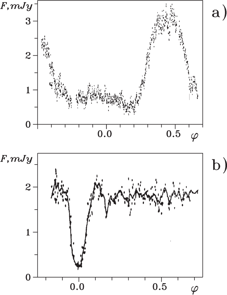
Fig. 6.—: Observed light curves for the dwarf novae: (a) VW Hyi, with the characteristic hump in the light curve, but without an eclipse [31], and (b) AC Cnc, with an eclipse, but without the hump [33].

(2) Many dwarf novae show an obvious hump in their light curve, but without any traces of an eclipse. One example of such a system is VW Hyi [31] (Fig. 6a), which is a SU UMa binary. The relative and absolute amplitudes of its light curve humps vary from cycle to cycle, and when the brightness of the system as a whole increases, the hump amplitude increases as well. If the hump is present, it usually occupies roughly half the orbital period, and the beginning and end of the hump occur at about the same orbital phase.

(3) In many objects whose orbital inclination $i$ differs strongly from zero, we observe a rapid drop in brightness in the light curve — an eclipse. As a rule, the eclipse occurs soon after the maximum of the main hump in the light curve (a typical example of such a system is U Gem [32]). The total duration of the eclipse is about 0.1 orbital cycles. The exact shape of the eclipse is usually slightly variable if different minimum for a single object are compared, but on average maintains its shape. Note that in some objects, the eclipses are irregular, however there is no hump in the light curve (for example, the system AC Cnc; Fig. 6b [33]), and in some eclipsing systems, the hump appears episodically.

(4) As a rule, if there is an eclipse, it occurs at the time of the maximum of the hump or just after it. However, in some nova-like stars (UX UMa type stars, similar to BV Cen and OY Car [17]), an additional intermediate hump is occasionally observed approximately between the end of the main hump and the beginning of the following one. This intermediate hump usually has more moderate brightness than the main hump, and its shape and amplitude are very variable. The beginning and end of both the main and the intermediate humps are repeatable with high accuracy.

(5) Five dwarf novae whose orbital inclinations are close to $90^{\circ}$ (Z Cha, OY Car, V2051 Oph, HT Cas, and IP Peg) have a very specific eclipse — a double eclipse. Both the ingress and egress of the eclipse occur in two stages, with the egress usually significantly longer than the ingress. Such double eclipses provide a large amount of information about the system, and are therefore objects of intense study. The shape of double eclipses can change from cycle to cycle. Here, it is obvious that two bright sources are eclipsed: the first sharp decrease in brightness is the eclipse of the white dwarf, after which, as usually assumed, follows the eclipse of the hot spot. After a more or less flat minimum, we observe the egress of the white dwarf eclipse followed by the extended egress of the hot-spot eclipse. The phase of the hot-spot eclipse egress changes from cycle to cycle. The phase of the primary minimum is highly stable in all objects.

In spite of the variety of the shapes of these light curves, their main features can be qualitatively well reproduced in the framework of our gas–dynamical model, with an energy release zone outside the accretion disk. Figures 7–11 present observed and theoretical light curves for cataclysmic variables with the most characteristic properties. We emphasize that we have limited our treatment to a qualitative comparison of the synthesized and observed light curves. The parameters of the binary systems used in our photometric calculations are summarized in the Table 1.

		Z Cha	U Gem	RW Tri	OY Car
Common system parameters
$q$	Mass ratio	4.95	2.2	1.2	9.8
$i$	Orbit incl.	$80^{\circ}$	$72^{\circ}$	$74^{\circ}$	$83^{\circ}$
Mass-losing star
$T_{rd}$	Temperature	4500 K	3100 K	3700 K	3000 K
Accretor
$R_{wd}$	Radius	0.0158$a$	0.0163$a$	0.0104$a$	0.0107$a$
$T_{wd}$	Temperature	33000 K	28000 K	45000 K	35000 K
Accretion disk
$R_{d}$	Radius	0.395$a$	0.32$a$	0.233$a$	0.354$a$
$h_{d}$	Thickness	0.013$a$	0.034$a$	0.028$a$	0.014$a$
$T_{d}$	Temperature	2300 K	3000 K	3400 K	2500 K
Bulge
$a_{b}$	Large semiaxe	0.103$a$	0.223$a$	0.152$a$	0.071$a$
$c_{b}$	Small semiaxe	0.013$a$	0.034$a$	0.032$a$	0.016$a$
$\alpha_{b}$	Azimuth	$14^{\circ}$	$14^{\circ}$	$22^{\circ}$	$25^{\circ}$
$T_{up}$	Temperature	7100 K	4300 K	37000 K	7500 K
	of upper part
$T_{down}$	Temperature	21000 K	17000 K	17000 K	12500 K
	of down part

Table 1:: The parameters of the binary systems used in photometric calculations

3.2.1 Systems with a double eclipse

The most interesting cases from the point of view of verifying the applicability of our model to the analysis of close binary systems are cataclysmic variables with double eclipses. We chose one such system — Z Cha — as a basis for our calculations of the flow pattern of matter in our gas–dynamical model (Section 2). When constructing the theoretical light curve for this system, we fixed the ratio of the component masses, orbital inclination, temperature of the normal star, and radius of the accretion disk. We fit the parameters of the white dwarf (its radius and temperature, and the thickness of the outer edge of the accretion disk) and also the parameters of the bulge in order to obtain the best qualitative agreement with the observed light curve (Fig. 7a), which we took from [9]. Figure 7b shows the theoretical light curve calculated for the parameter values listed in the Table 1.

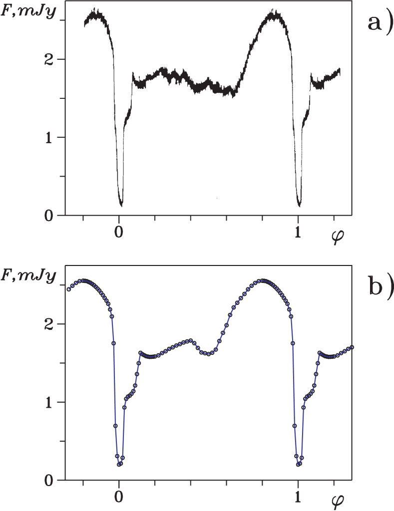
Fig. 7.—: Cataclysmic variable with a double eclipse: (a) observed [9] and (b) theoretical light curves for the dwarf nova Z Cha in the $V$ filter.

A visual comparison of the curves in Fig. 7 shows that they are in good qualitative agreement. We can see in the theoretical curve essentially all the main features in the observed light curve of Z Cha. The egresses for both the white dwarf and bulge eclipse are well followed. The modest minimum at phase $\varphi=0.5$ is associated with the ellipsoidality effect of the red dwarf. Note that the fitted parameters for the white dwarf $R_{wd}=0.0158a$ and $T_{wd}=33000$ K are close to the values derived earlier in [26], $R_{wd}=0.0116a$ and $T_{wd}=17000\div 24000$ K.

3.2.2 Systems with a single hump and ordinary eclipse

The shape of the observed light curve in the system U Gem (Fig. 8a), in contrast to the light curve for Z Cha, does not show any trace of the eclipse of the white dwarf, and corresponds to the eclipse only of the region of energy release (the bulge). Using the parameters obtained earlier for U Gem ($q=2.2$, $T_{rd}=3100$ K (SP M4 V), $R_{d}=0.32a$ [7]), we were able to obtain good qualitative agreement between the observed and theoretical light curves (Figs. 8a, 8b) purely by increasing the previously proposed inclination value $i=69^{\circ}\pm 1^{\circ}$ to $72^{\circ}$. The remaining parameters for the photometric light curve are presented in the Table 1. As expected, the bulge dominates the total brightness of the system, and variations in its brightness with orbital phase determine the appearance of the light curve. At this orbital inclination, the white dwarf is not eclipsed, in spite of the fact that the red dwarf is larger than in the Z Cha system (the radius of the red dwarf in U Gem is $0.3a$, while the size of the red dwarf in Z Cha does not exceed $0.23a$).

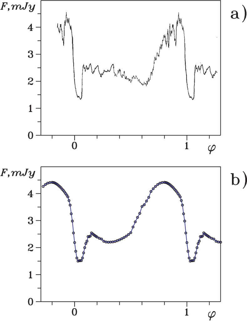
Fig. 8.—: System with a single hump and an ordinary eclipse: (a) observed [32] and (b) theoretical light curves of the dwarf nova U Gem in the $V$ filter.

Fig. 8c.—: Separate dependences of the brightnesses of the red dwarf (1), white dwarf (2), accretion disk (3), and bulge (4) on orbital phase for Fig. 8b

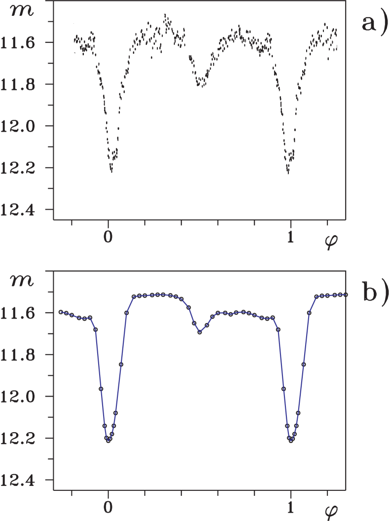
Fig. 9.—: Cataclysmic variable with an anomalously placed hump: (a) observed [34] and (b) theoretical light curves of the dwarf nova RW Tri in the $K$ filter.

3.2.3 Systems with anomalous hump positions

The classical light curves presented above can be qualitatively rather well described by our model for flow without a hot spot. Note also that our results are in good agreement with calculations for standard models with a hot spot, which were developed especially to interpret such light curves. Therefore, for our further verification of the adequacy of our shock-wave flow model, we will consider light curves that could not be explained in the framework of standard hot-spot models. These correspond to systems displaying an extended hump at phase 0.5 and systems in which the eclipse begins on the ascending branch of the hump.

RW Tri is one of the most remarkable cataclysmic variables in this context. This system is a so-called anti-flare star, or UX UMa type star. A hump is clearly visible in both the optical and infrared light curves of RW Tri after the egress of the white dwarf eclipse (Fig. 9a [34], 10a [16]). The main parameters of this system were derived primarily from the width of the white dwarf eclipse [7, 16], which is $\Delta\varphi=0.078\pm 0.002$ of the orbital period; $q=5$ for $i=90^{\circ}$, $q=2$ for $i=75^{\circ}$, and $q=0.8$ for $i=70^{\circ}$. According to the studies of Horne and Stiening [16], the radius of the disk is rather large, and reaches nearly 60is the distance between the inner Langrange point and the center of mass of the white dwarf. The red dwarf has spectral type M0 V, corresponding to a surface temperature of $T_{rd}\sim 3700$ K.

Figure 9b presents the theoretical light curve in the $K$ filter calculated for parameters close to those determined earlier for the system: $q=1.2$ for $i=74^{\circ}$ and $R_{d}=0.233a$ ($\sim 0.45\xi$). The remaining model parameters are given in the Table 1. We assumed that the appearance of the hump after the egress of the white dwarf eclipse could be due to strong emission from the side of the bulge turned toward the incident stream. Therefore, we adopted the model temperature of the bulge on this side to be $T_{up}\sim 37000$ K, and on the other side to be about half this, $T_{down}\sim 17000$ K. The calculated light curve (fig. 9b) is in good agreement with the observed curve. In particular, we can clearly see the increase in brightness during the eclipse egress above the brightness level during the eclipse ingress. Figure 9c presents part of the theoretical $K$ light curve of RW Tri near the eclipse of the bulge (in intensity units). The shape of the minimum is determined primarily by the wide brightness minimum of the red dwarf, which is associated with the passage into the line of sight of cold areas on the back hemisphere of the red dwarf that have not been heated by the white dwarf, and also with the eclipse of the unevenly heated bulge, on which the narrower eclipse of the disk is superposed (Fig. 9d).

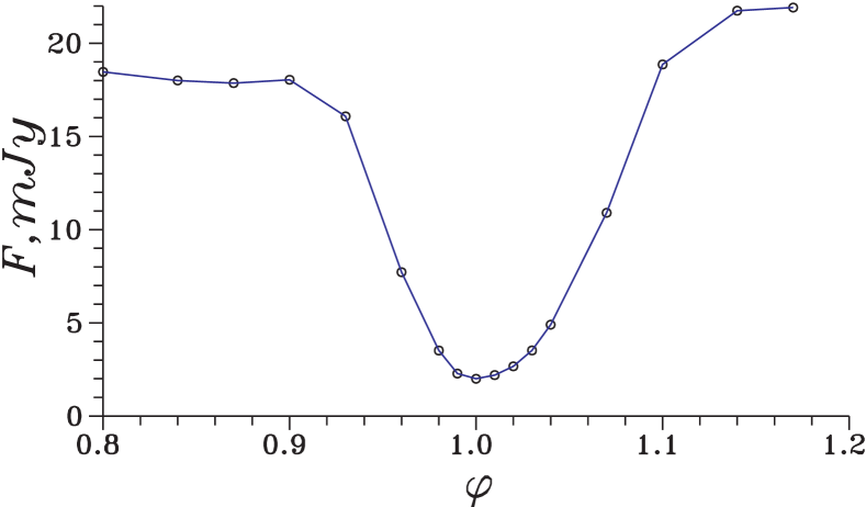
Fig. 9c.—: Part of the theoretical $K$ light curve for RW Tri in the region of the bulge eclipse.

Fig. 9d.—: Separate dependences of the brightnesses of the red dwarf (1), white dwarf (2), accretion disk (3), and bulge (4) on orbital phase for Fig. 9b.

Figure 10 presents the observed [16] and theoretical light curves for this system (also in intensity units) at optical wavelengths (the $B$ filter). When constructing the model curve for the $B$ filter, we used somewhat different parameters for the bulge: $a_{b}=0.163a$, $c_{b}=0.029a$, and $\alpha_{b}=18^{\circ}$; the brightness temperature on the side of the incident stream was decreased to $T_{up}\sim 23000$ K, while the temperature on the opposite side remained the same. It is clear that the qualitative agreement between the model and observed light curves is maintained at optical wavelengths.

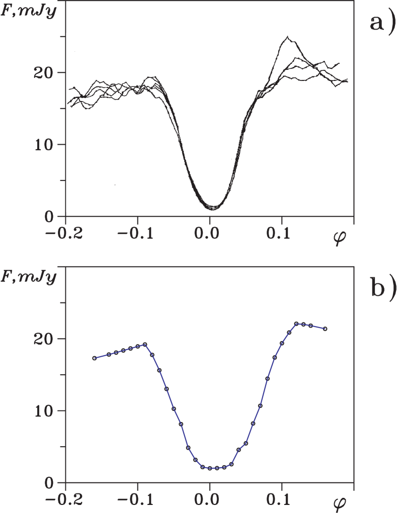
Fig. 10.—: Cataclysmic variable with an anomalously placed hump: (a) observed [16] and (b) theoretical light curves of RW Tri in the $B$ filter in the region of the bulge eclipse.

3.2.4 Systems with an intermediate hump in their light curves

Even more interesting from the point of view of testing our model’s ability to describe ”irregularities” in the light curves of cataclysmic variables is the light curve of OY Car, which is characterized by the episodic appearance of a secondary hump with lower amplitude near orbital phase $\varphi\sim 0.5$ (Fig. 11a). In the framework of our model, this can also be explained by appropriate ratios of the luminosities of the model components in a system with $i$ close to $90^{\circ}$.

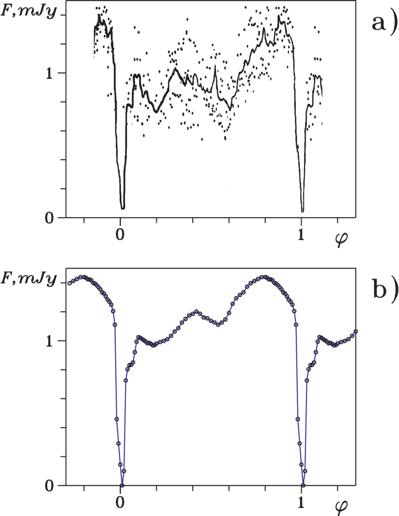
Fig. 11.—: System with an intermediate hump in the light curve: (a) observed [17] and (b) theoretical light curves of the dwarf nova OY Car in the $V$ filter.

Numerous previous studies of the region of the eclipse of the white dwarf indicate the parameters for OY Car [7] to be $q=9.8\pm 0.3$, $i=83^{\circ}$, Sp M5 V ($T_{rd}\sim 3000$ K), and $R_{d}=0.355a$. We fixed the values for $q$, $i$, $T_{rd}$, and $R_{d}$ and fitted the remaining parameters in order to qualitatively reproduce the main features of the light curve of OY Car (see Table 1). The resulting theoretical light curve is presented in Fig. 11b, and is clearly in good qualitative agreement with the observed curve. The secondary hump in the light curve is associated with heating of the bulge by radiation from the white dwarf.

Fig. 11c.—: Separate dependences of the brightnesses of the red dwarf (1), white dwarf (2), accretion disk (3), and bulge (4) on orbital phase for Fig. 11b.

Figure 11c shows the contributions of individual components of the system to the overall flux at various orbital phases. The white dwarf makes the largest contribution to the total flux at virtually all phases, except the phase when it is eclipsed by the red dwarf and phases when the line of sight intersects the hottest region of the bulge ($\varphi\sim 0.7-0.9$). The contribution of the disk outside of eclipse is somewhat smaller. The flux from the normal star at the maximum is nearly a third the flux of the white dwarf. Variations in the brightness of the red dwarf are primarily associated with the reflection effect, i.e., the heating of the red dwarf by radiation from the hot white dwarf. The most interesting variations are the orbital-phase variations of the bulge, associated with its turning relative to the line of sight. The secondary, smaller, hump at phase $\varphi\sim 0.4$ corresponds to the situation when the line of sight intersects the part of the bulge that is higher than the upper edge of the disk, and is heated by both radiation from the white dwarf and the shock interaction with the common envelope gas.

There is no doubt that our results represent only a crude, rather schematic attempt to explain the observed features of the light curves of cataclysmic variables by invoking the presence of an optically thick formation with substantial geometrical size outside the accretion disk — a shock wave at the edge of the gaseous stream flowing around the disk. However, even in the framework of our simplified photometric model, we are able to obtain a variety of light curves that reflect rather fully all the main features of the brightness variations of cataclysmic variables.

4 Conclusion

Our three-dimensional numerical simulations of the gas–dynamical flow of matter in a cataclysmic binary system similar to Z Cha provide evidence that there is no shock interaction between the stream of matter flowing from $L_{1}$ and the accretion disk in a self-consistent solution for this system. We first suggested that this was the case based on our studies of low-mass X-ray binary systems [24, 25], however at that time, the question of the applicability of our model to other types of binary systems remained open. Our results here have confirmed that the solutions for different types of semidetached binary systems are qualitatively similar, indicating that the behavior ontained in our simulations is universal in these systems.

Summarizing the main properties of the resulting flow patterns in our model, we first note that the rarified common-envelope gas significantly influences the structure of the gas flows in a non-magnetic system in a steady-state flow regime. The common-envelope gas interacts with the stream flowing from the vicinity of $L_{1}$ and deflects this stream, so that its interaction with the outer edge of the accretion disk is shock-free (tangential), and no hot spot is formed in the disk. At the same time, the interaction of the common-envelope gas with the stream leads to the formation of an extended shock wave along the edge of the stream. One of the characteristic properties of this shock is its variable intensity along its length, with the main energy release occurring in a compact region of the shock near the accretion disk.

We compared synthetic light curves based on our flow model with a variety of observed light curves for cataclysmic binary systems. These comparisons show that our flow model without a hot spot can describe the light curves rather well. In addition, we are able to create synthesized light curves that are in good agreement with the observed curves in cases when this is not possible in the framework of standard models with an accretion disk hot spot. We, therefore, conclude that this observational confirmation of the adequacy of our self-consistent, gas–dynamical flow model provides a firm basis to prefer this model over standard hot-spot models in the investigation of semidetached close binary systems.

This work was supported by the Russian Foundation for Basic Research (project codes 96-02-16140, 96-02-19017) and by the Program of Support to Leading Scientific Schools of the Russian Federation (project no. 96-15-96489).

REFERENCES

[1] Kopal, Z., Annal d’Astrophys., 1955, 18, 379

[2] Kopal, Z., 1959, Close Binary Systems. Chapmen & Hall, London

[3] Struve, O., 1950, Stellar Evolution. Princeton Univ., Princeton

[4] Sahade, J., 1960, in Stellar Atmospheres, ed. J.L. Greenstein. Univ. of Chicago Press, Chicago, p. 466

[5] Batten, A., 1973, Binary and Multiple Systems of Stars. Pergamon Press, Oxford

[6] Shore, S., Livio, M., van Den Heuvel, E., 1994, Interacting Binaries. Springer-Verlag, Berlin-Budapest

[7] Cherepashchuk, A.M., Katysheva, N.A., Khruzina, T.S., Shugarov, S.Yu., 1996, Highly Evolved Close Binary Stars. Catalog. Gordon & Breach, London

[8] Hack, M., La Dous, C., 1993, Cataclysmic variables and related objects. (NASA SP-507, Monograph series on nonthermal phenomena in stellar atmospheres). U.S.Gov.Printing Office, Washington

[9] Wood, J., Horne, K., Berriman, G., Wade, R., O’Donoghue, D., Warner, B., 1986, MNRAS, 219, 629

[10] Dmitrienko, E.S., Matvienko, A.N., Cherepashchuk, A.M., Yagola, A.G., 1984, Sov. Astron., 28, 180

[11] Smak, J., 1970, Acta Astron., 20, 312

[12] Matvienko, A.N., Cherepashchuk, A.M., Yagola, A.G., 1988, Sov. Astron., 32, 526

[13] Horne, K., 1985, MNRAS, 213, 129

[14] Horne, K., Cook, M.C., 1985, MNRAS, 214, 307

[15] Horne, K., March, T.R., 1986, MNRAS, 218, 761.

[16] Horne, K., Stiening, R.F., 1985, MNRAS, 216, 933

[17] Schoembs, R., Hartmann, K., 1983, A&A, 128, 37

[18] Lubow, S.H., Shu, F.H., 1975, ApJ, 198, 383

[19] Marsh, T.R., Horne, K., 1988, MNRAS, 235, 269

[20] Marsh, T.R., Horne, K., 1990, ApJ, 349, 593.

[21] Molteni, D., Belvedere, G., Lanzafame, G., 1991, MNRAS, 249, 748

[22] Belvedere, G., Lanzafame, G., Molteni, D., 1993, A&A, 280, 525

[23] Lanzafame, G., Belvedere, G., Molteni, D., 1994, MNRAS, 267, 312

[24] Bisikalo, D.V., Boyarchuk, A.A., Kuznetsov, O.A., Chechetkin, V.M., 1997, Astron. Reports, 41, 786 (also available as astro-ph/9802004)

[25] Bisikalo, D.V., Boyarchuk, A.A., Kuznetsov, O.A., Chechetkin, V.M., 1997, Astron. Reports, 41, 794 (also available as astro-ph/9802039)

[26] Goncharskii, A.V., Cherepashchuk, A.M., Yagola, A.G., 1985, Ill-posed Problems in Astrophysics. Nauka, Moscow (in russian)

[27] Landau, L.D., Lifshitz, E.M., 1959, Fluid Mechanics. Pergamon, Elmsford

[28] Khruzina, T.S., 1992, Sov. Astron., 36, 29

[29] Khruzina, T.S., Cherepashchuk, A.M., 1994, Astron. Reports, 38, 386

[30] Khruzina, T.S., Astron. Reports, in press

[31] Warner, B., 1975, MNRAS, 170, 219

[32] Warner, B., Nather, R.E., 1971, MNRAS, 152, 219

[33] Yamasaki, A., Okazaki, A., Kitamura, M., 1983, PASJ, 35, 423

[34] Longmore, A.J., Lee, T.J., Alleu, D.A., Adams, D.J., 1981, MNRAS, 195, 825