Joint estimation of cosmological parameters from CMB and IRAS data

Abstract

Observations of large scale structure (LSS) and the Cosmic Microwave Background (CMB) each place separate constraints on the values of cosmological parameters. We calculate a joint likelihood based on various CMB experiments and the IRAS 1.2Jy galaxy redshift survey and use this to find an overall optimum with respect to the free parameters. Our formulation self-consistently takes account of the underlying mass distribution, which affects both the CMB potential fluctuations and the IRAS redshift distortion. This not only allows more accurate parameter estimation, but also removes the parameter degeneracy which handicaps calculations based on either approach alone. The family of Cold Dark Matter (CDM) models analysed corresponds to a spatially-flat universe with an initially scale-invariant spectrum and a cosmological constant. Free parameters in the joint model are the mass density due to all matter (${\Omega_{\rm m}}$), Hubble’s parameter ($h=H_{0}/100{\rm\ km\ s^{-1}}{\rm Mpc}^{-1}$), the quadrupole normalisation of the CMB power spectrum ($Q$) in $\mu$K, and the IRAS light-to-mass bias (${b_{\rm iras}}$). Throughout the analysis, the baryonic density ($\Omega_{b}$) is required is to satisfy the nucleosynthesis constraint $\Omega_{b}h^{2}=0.024$. Results from the two data sets show good agreement, and the joint optimum lies at ${\Omega_{\rm m}}=0.39$, $h=0.53$, $Q=16.96$ $\mu$K, and ${b_{\rm iras}}=1.21$. The 68 per cent confidence intervals are: $0.29<{\Omega_{\rm m}}<0.53$, $0.39<h<0.58$, $15.34<Q<17.60$, and $0.98<{b_{\rm iras}}<1.56$. For the above parameters the normalisation and shape of the mass power-spectrum are $\sigma_{8}=0.67$ and $\Gamma=0.15$, and the age of the Universe is $16.5$ Gyr.

1 Introduction

Astronomical observations allow us to evaluate cosmological models, and determine likely values for the parameters within them. As the variety and depth of these observations have improved, so too have the techniques for comparing them against theoretical predictions.

Observations of anisotropies in the Cosmic Microwave Background (CMB) provide one of the key constraints for cosmological models and a significant quantity of experimental data already exists. By comparing the power spectrum of the CMB fluctuations derived from these experiments with the power spectra predicted by different cosmological models it is possible to set constraints on the value of certain cosmological parameters (e.g. Hancock et al. (1998), Lineweaver et al. (1997), and references therein).

Galaxy redshift surveys, mapping large scale structure (LSS), provide another cosmologically important set of observations. The clustering of galaxies in redshift-space is systematically different from that in real-space (Kaiser (1987)). The mapping between the two is a function of the underlying mass distribution, in which the galaxies are not only tracers, but also velocity test particles (Lahav (1996)). Many techniques have been developed for estimating this mapping (Yahil et al. (1991); Kaiser et al. (1991)). Statistical quantities can be generated for a given cosmology and these used to constrain model parameters through comparison with survey data (Fisher, Scharf & Lahav (1994); Cole et al. (1995); Heavens & Taylor (1995); Fisher & Nusser (1996); Willick et al. (1997)).

Estimates derived separately from each of these two data sets have problems with parameter degeneracy. In the analysis of LSS data, there is uncertainty as to how well the observed light distribution traces the underlying mass distribution. The light-to-mass linear bias, $b$, introduced to account for this uncertainty, affects the value of many central cosmological parameters, and makes any identified optimum degenerate (Strauss & Willick (1995)). Similarly, on the basis of CMB data alone, there is considerable degeneracy (Bond et al. 1995c ) between ${h}=H_{0}/100{\rm\ km\ s^{-1}}{\rm Mpc}^{-1}$ and the energy density ${\Omega_{\Lambda}}$ due to the cosmological constant (Carroll, Press & Turner (1992)). This leads to poor estimation of the baryon (${\Omega_{\rm b}}$) and total mass (${\Omega_{\rm m}}$) densities (Lineweaver et al. (1997)).

In this letter, we combine results from a bandpower approach covering a range of CMB experiments, with a likelihood analysis of the IRAS 1.2Jy survey, performed in spherical harmonics. We present a self-consistent formulation of CMB and LSS parameter estimation. In particular, our method expresses the effects of the underlying mass distribution on both the CMB potential fluctuations and the IRAS redshift distortion. This breaks the degeneracy inherent in an isolated analysis of either data set, and places tight constraints on several cosmological parameters. Indeed, it is unsurprising that the two data sets are complementary, given that they sample our universe at extreme ends of its evolution. For simplicity, we restrict our attention to inflationary, Cold Dark Matter (CDM) models, assuming a flat universe with linear, scale-independent biasing. Other recent studies which combine CMB and LSS include Gawiser & Silk (1998) and Eisenstein, Hu & Tegmark (1998).

2 CMB Parameter Estimation

2.1 Experimental Data

Since the discovery of CMB fluctuations by the COBE satellite (Smoot et al. (1992); Bennett et al. (1996)), several other experiments have also measured CMB anisotropies over a wide range of angular scales. These experiments include ground-based beam-switching experiments such as Tenerife (Hancock et al. (1997, 1994)), Python (Ruhl et al. (1995)), South Pole (Gundersen et al. (1995)) and Saskatoon (Netterfield et al. (1997)); balloon-borne instruments such as ARGO (De Bernardis et al. (1994)), MAX (Tanaka et al. (1996)), and MSAM (Cheng et al. (1994, 1996)) and the ground-based interferometers CAT (Scott et al. (1996)) and OVRO (Leitch et al. (1998)).

These observations have resulted in a first estimate of the CMB power spectrum and they are discussed in more detail by Hancock et al. (1998). In particular, Hancock et al. display the window function $W_{l}$ for each experiment and convert the level of anisotropy observed in each case to flat bandpower estimates $(\Delta T_{l}/T)\pm\sigma$ centered on the effective multipole $l_{\rm eff}$ of the corresponding window function (see below). The resulting CMB data points are plotted in Fig. 1, together with their 68 per cent confidence limits. These confidence limits have been obtained using likelihood analyses and hence incorporate uncertainties due to random errors, sampling variance (Scott, Srednicki and White (1994)) and cosmic variance (Scaramela & Vittorio (1990, 1993)). A discussion of possible additional uncertainties due to contamination by foreground emission is given by Rocha et al. (1998).

The data points plotted in Fig. 1 differ slightly from those given in Hancock et al. (1998) as follows. The old Python point has been replaced by two new points corresponding to the Py III_S and Py I, Py II and Py III_L observations respectively (Platt et al. (1997)). The Tenerife point has been updated following the analysis of the full two-dimensional data-set and a detailed treatment of atmospheric effects (Gutierrez (1997)). The Saskatoon points have been increased by 5 per cent, as suggested by the recent investigation of systematic calibration errors in the Saskatoon experiment (Leitch, private communication). We have added the results from the second CAT field, reported in Baker et al. (1998) and also the OVRO point reported by Leitch et al. (1998).

2.2 Method

Temperature fluctuations in the CMB are usually described in terms of the spherical harmonic expansion

$$\frac{\Delta T(\theta,\phi)}{T}=\sum_{l=0}^{\infty}\sum_{m=-l}^{l}a_{lm}\,Y_{lm}(\theta,\phi)\ ,$$ (1)

from which we define the ensemble-average CMB power spectrum $C_{l}=\langle|a_{lm}|^{2}\rangle$. Alternatively, we may describe the fluctuations in terms of their autocorrelation function

$$C(\theta)=\frac{1}{4\pi}\sum_{l=2}^{\infty}\,(2l+1)\,C_{l}\,P_{l}(\cos\theta)\ .$$ (2)

The power in the CMB fluctuations observed by an experiment with window function $W_{l}$ is then given by

$$C_{\rm obs}(0)=\left\langle{\left(\frac{\Delta T_{\rm obs}}{T}\right)^{2}}\right\rangle=\frac{1}{4\pi}\sum_{l=2}^{\infty}\,(2l+1)\,C_{l}\,W_{l}\ ,$$ (3)

and for each experiment we define the flat bandpower by

$${\frac{\Delta T_{l}}{T}}=\sqrt{{C_{\rm obs}(0)}\over{I(W_{l})}}\ ,$$ (4)

where $I(W_{l})$ is defined (Bond 1995a ; Bond 1995b ) as

$$I(W_{l})=\sum_{l=2}^{\infty}\frac{(l+\textstyle{\frac{1}{2}})}{l\,(l+1)}\ W_{l}\ .$$ (5)

This flat bandpower estimate is centred on the effective multipole

$$l_{\rm eff}={{I(l\,W_{l})}\over{I(W_{l})}}\ .$$ (6)

We wish to compare these bandpower estimates with those predicted by different cosmological models. Varying the values of model parameters, we calculate corresponding, predicted CMB power spectrum $C_{l}$, using the Boltzmann code of Seljak & Zaldarriaga (1996). This is then used to calculate the predicted flat bandpower $\Delta T_{l}$ for each experiment. The chi-squared statistic for a given set of parameter values, ${\vec{\alpha}}_{\rm cmb}$, is then

$$\chi^{2}({\vec{\alpha}}_{\rm cmb})=\sum_{i=1}^{N_{\rm d}}{\frac{1}{\sigma_{i}^{2}}}{{\left(\left[\Delta T_{l}^{\rm obs}\right]_{i}-\left[\Delta T_{l}^{\rm pred}({{\vec{\alpha}}_{\rm cmb}})\right]_{i}\right)}^{2}}\ ,$$ (7)

where $N_{\rm d}$ is the number of CMB data points plotted in Fig. 1 (20 in this analysis). Moreover, since the CMB data points plotted in Fig. 1 were chosen such that no two bandpower estimates come from experiments which observed overlapping patches of sky and had overlapping window functions, we may consider them as independent estimates of the CMB power spectrum. As the cosmic variance has already been taken into account in deriving the flat bandpower estimates, the likelihood function is given simply by ${\cal L}_{\rm cmb}\propto e^{-\chi^{2}/2}$.

As mentioned above, we assume that the Universe is spatially flat, and that there are no tensor contributions to the CMB power spectrum. We take the primordial scalar perturbations to be described by the Harrison-Zel’dovich power spectrum for which ${n_{\rm s}}=1$, and further assume that the optical depth to the last scattering surface is zero.

The normalisation of the CMB power spectrum is determined by $Q$, which gives the strength of the quadrupole in $\mu K$, such that

$$C_{2}={{{4\pi}\over{5}}\,{{\left({Q}\over{T_{0}}\right)}^{2}}}\ ,$$ (8)

where $T_{0}$ is the average CMB temperature. The expansion rate of the Universe is given by Hubble’s parameter $h=H_{0}/100{\rm\ km\ s^{-1}}{\rm Mpc}^{-1}$, while ${\Omega_{\rm cdm}}$ and ${\Omega_{\rm b}}$ denote the density of the Universe in CDM and the baryons respectively, each in units of the critical density. Given that we assume a flat universe, but investigate models where

$${\Omega_{\rm m}}\equiv({\Omega_{\rm cdm}}+{\Omega_{\rm b}})<1\ ,$$ (9)

the shortfall is made up through a non-zero cosmological constant $\Lambda$ such that

$${\Omega_{\Lambda}}=1-{\Omega_{\rm m}}={{\Lambda}\over{3{H_{0}^{2}}}}\ .$$ (10)

Furthermore, we restrict our attention to models that satisfy the nucleosynthesis constraint $\Omega_{b}h^{2}=0.024$ (Tytler, Fan & Burles (1996)). Thus we consider the reduced set of CMB parameters

$${\vec{\alpha}}_{\rm cmb}\equiv\{Q,h,{\Omega_{\rm cdm}}\}\ .$$ (11)

In Section 4, we derive a set of joint parameters linking these to the IRAS parameter set.

3 IRAS Parameter Estimation

3.1 IRAS 1.2Jy Survey

The IRAS surveys are uniform and complete down to Galactic latitudes as low as $\pm 5^{\circ}$ from the Galactic plane. This makes them ideal for estimating whole-sky density and velocity fields. Here, we use the 1.2 Jy IRAS survey (Fisher et al. (1995)), consisting of 5313 galaxies, covering 87.6% of the sky with the incomplete regions being dominated by the 8.7% of the sky with $|b|<5^{\circ}$.

In principle, the method we are using can be extended to account explicitly for the incomplete sky coverage. However, we adopt the simpler approach of smoothly interpolating the redshift distribution over the missing areas (Yahil et al. (1991)). The effects of this interpolation on the computed harmonics have been shown to be negligible (Lahav et al. (1994)).

3.2 Method

In this letter, we assume linear, scale-independent biasing, where ${b_{\rm iras}}$ measures the ratio between fluctuations in the IRAS galaxy distribution and the underlying mass density field:

$${\left({{\delta\rho}/{\rho}}\right)}_{\rm iras}={b_{\rm iras}}\,{\left({{\delta\rho}/{\rho}}\right)_{\rm m}}\ .$$ (12)

We note that biasing may be non-linear, stochastic, non-local, scale-dependent, epoch-dependent and type-dependent (e.g. Dekel and Lahav (1998), Tegmark & Peebles (1998), Pen (1998), Bagla (1998), Blanton et al. (1998), and references therein). For a linear bias parameter, ${b_{\rm iras}}$, the velocity and density fields in linear theory (Peebles (1980)) are linked by a proportionality factor ${\beta_{\rm iras}}\equiv{{{\Omega_{\rm m}}^{0.6}}/{{b_{\rm iras}}}}$, such that

$$\nabla\cdot{\bf v}=-H_{0}\,{\beta_{\rm iras}}\,\left({{\delta\rho}/{\rho}}\right)_{\rm m}$$ (13)

Statistically, the fluctuations in the real-space galaxy distribution can be described by a power spectrum, ${P_{\rm R}(k)}$, which is determined by the rms variance in the observed galaxy field, measured for an 8$\ {h^{-1}\rm Mpc}$ radius sphere (${\sigma_{8,{\rm iras}}}$) and a shape parameter (e.g. $\Gamma$ in equation 19). The observed ${\sigma_{8,{\rm iras}}}$ is related to the underlying ${\sigma_{8}}$ for mass through the bias parameter, such that ${\sigma_{8,{\rm iras}}}={b_{\rm iras}}\,{\sigma_{8}}$.

The approach we use in this letter follows Fisher, Scharf & Lahav (1994; hereafter FSL), and we include here only a brief introduction to our technique. FSL provides a detailed description of the spherical harmonic approach to parameter estimation. A flux-limited, redshift-space density field can be decomposed into spherical harmonics $Y_{lm}$, with coefficients

$$a_{lm}^{\rm S}=\sum\limits_{i=1}^{N_{\rm g}}f(s_{i})\,Y_{lm}\left(\hat{\bf s}_{i}\right)\ ,$$ (14)

where $N_{\rm g}$ is the number of galaxies in the survey, and $f(s)$ is an arbitrary radial weighting function—this process is analogous to Fourier decomposition, but instead using spherical basis functions. The sum over galaxies in this equation can be rewritten as a continuous integral of the density fluctuation field $\delta({\bf s})$ over redshift-space:

$$a_{lm}^{\rm S}=\int d^{3}{\bf s}\,\,\phi(r)\,f(s)\,\left[1+\delta_{S}({\bf s})\right]\,Y_{lm}(\hat{\bf s})\ ,$$ (15)

where $\phi(r)$ is the radial selection function of the survey, evaluated at the real-space distance of the $i^{\rm th}$ galaxy.

As detailed in FSL, assuming the perturbations introduced by peculiar velocities are small, the expected linear theory values for the harmonic coefficients are

$${\left\langle{\left|a_{lm}^{\rm S}\right|}^{2}\right\rangle}_{\rm LT}={2\over\pi}\,{\int\limits_{0}^{\infty}dk\,\,{k^{2}}\,{P_{\rm R}(k)}\,{{\left|{\Psi_{l}^{\rm R}(k)+{\beta_{\rm iras}}\Psi_{l}^{\rm C}(k)}\right|}^{2}}}\ .$$ (16)

Here, $\Psi^{\rm R}$ is the real-space window function, while ${\beta_{\rm iras}}\Psi^{\rm C}$ is a “correction” term which embodies the redshift distortion.

For a given set of cosmological parameters, redshift-space harmonics $a^{j}_{lm}$ can be calculated for different weighting functions $f^{j}(r)$, ${j=1,...,N}$. If the underlying density field is Gaussian, on the basis of the coefficients predicted in equation 16, the likelihood of the survey harmonics can be calculated as

$${\cal L}_{\rm iras}\propto{{\left|{\bf A}\right|}^{-{{1}\over{2}}}}\,{{\rm exp}\left({{-{{1}\over{2}}}\left[{{\vec{a}}^{\rm T}}\,{\bf A}^{-1}\,{\vec{a}}\right]}\right)}\ .$$ (17)

Here $\vec{a}$ is the vector of observed harmonics for different shells and ${\bf A}$ is the corresponding covariance matrix, which depends on the predicted harmonics. In addition to the ${\langle|a_{lm}^{\rm S}|\rangle}_{\rm LT}$ from equation 16, these predicted harmonics will also have a shot-noise contribution ${\langle|a_{lm}^{\rm S}|\rangle}_{\rm SN}$ due to the discreteness of survey galaxies. Note that the argument of the exponent in equation 17 is simply $(-\chi^{2}/2)$, and that here the normalisation of the likelihood function does depend on the free parameters (unlike in the CMB likelihood function).

In this letter, we follow FSL and use four Gaussian windows centered at 38, 58, 78, and 98 $\ {h^{-1}\rm Mpc}$ each with a dispersion of 8 $\ {h^{-1}\rm Mpc}$. For each window, we compute the corresponding weighted redshift harmonics for the IRAS 1.2Jy catalog, and use these to determine the likelihood of a given set of parameter values. Since our analysis is valid only in the linear regime, we restrict the likelihood computation to $l_{\rm max}=10$ (corresponding to 120 degrees of freedom). Hence, the IRAS likelihood function has a parameter vector

$${\vec{\alpha}}_{\rm iras}\equiv\{{\beta_{\rm iras}},{\sigma_{8,{\rm iras}}},\Gamma\}\ .$$ (18)

Again, the linkage between these and the CMB parameters is discussed in section 4 below.

4 Joint analysis

Given the large number of parameters available between the two models, it is important both to find links for joint optimisation, and to decide which parameters can be frozen. From section 3, we have six variables between the two models: {$Q$, ${h}$, ${\Omega_{\rm cdm}}$, ${\beta_{\rm iras}}$, ${\sigma_{8,{\rm iras}}}$, $\Gamma$}. These can be reduced further by expression in terms of core cosmological parameters. The IRAS normalisation can be calculated as ${\sigma_{8}}\equiv f({\Omega_{\rm m}},Q,\Gamma)$ (Bardeen et al. (1986); Efstathiou, Bond & White (1995)), while the CDM shape parameter is well approximated (Sugiyama (1995)) by

$$\Gamma={\Omega_{\rm m}}\,{h}\ {\rm exp}\left({-{\Omega_{\rm b}}\left[1+{{\sqrt{{h}/0.5}}\over{{\Omega_{\rm m}}}}\right]}\right)\ .$$ (19)

Meanwhile, we have shown above that ${\Omega_{\rm m}}={\Omega_{\rm cdm}}+{\Omega_{\rm b}}$, ${\beta_{\rm iras}}=\Omega_{\rm m}^{0.6}/{b_{\rm iras}}$, and ${\sigma_{8,{\rm iras}}}={\sigma_{8}}{b_{\rm iras}}$. Hence, the final, joint parameter space is

$${\vec{\alpha}}_{\rm joint}\equiv\{{h},Q,{\Omega_{\rm m}},{b_{\rm iras}}\}\ .$$ (20)

As the IRAS and CMB probe very different scales and hence are assumed to be uncorrelated, the joint likelihood is given by

$${\rm ln}\left({\cal L}_{\rm joint}\right)={\rm ln}\left({\cal L}_{\rm cmb}\right)+{\rm ln}\left({\cal L}_{\rm iras}\right)\ .$$ (21)

5 Results

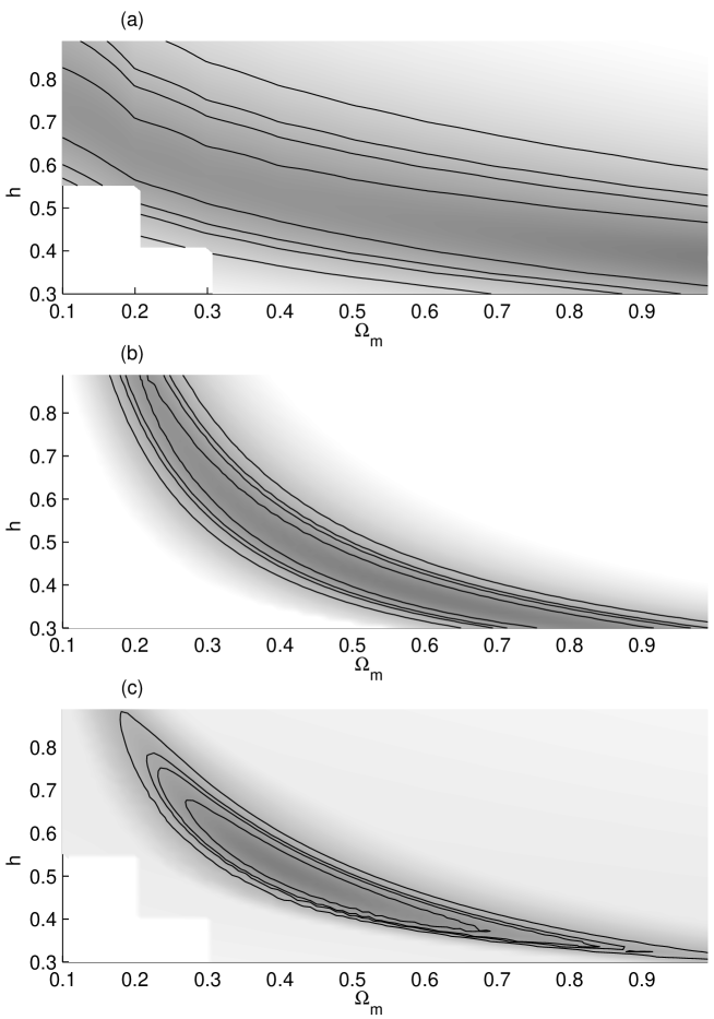
Figure 2: The likelihood function in the {${\Omega_{\rm m}}$, ${h}$}-plane, after marginalisation over $Q$ and ${b_{\rm iras}}$, for (a) CMB alone, (b) IRAS alone and (c) joint CMB and IRAS. The contours denote the 68, 90, 95 and 99 per cent confidence regions.

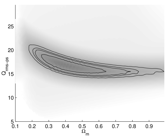
Figure 3: The joint CMB+IRAS likelihood function in the {${\Omega_{\rm m}}$, $Q$}-plane after marginalisation over ${h}$ and ${b_{\rm iras}}$. The contours denote the 68, 90, 95 and 99 per cent confidence regions.

The complementary nature of the two data sets is demonstrated in Fig. 2, which shows likelihood contours in the {${\Omega_{\rm m}}$, ${h}$}-plane after marginalising over $Q$ and ${b_{\rm iras}}$. The fundamental CMB-side degeneracy in {${\Omega_{\rm m}}$, ${h}$} is seen in the flat trough running across Fig. 2a. The IRAS degeneracy is in a different direction (Fig. 2b) and the two data sets agree well in the region where the lines of degeneracy overlap. Combining the two data sets breaks the degeneracy and leads to a well defined joint optimum (Fig. 2c). The joint CMB plus IRAS likelihood function in the {${\Omega_{\rm m}}$, $Q$}-plane and {${h}$, $Q$}-plane is plotted in Figs 3 & 4 respectively. In each case, a marginalisation has been performed over the other two parameters.

The joint likelihood (equation 21) was maximized with respect to the 4 free parameters (equation 20) using standard optimisation techniques (Press et al. (1992)) and the best fit parameters are shown in Table 1.

	Free parameters
${\Omega_{\rm m}}$	$0.39$	$0$.	$29$ $\,<\,$	${\Omega_{\rm m}}$ $\,<\,$	$0$.	$53$
$h$	$0.53$	$0$.	$39$ $\,<\,$	$h$ $\,<\,$	$0$.	$58$
$Q$ ($\mu$K)	$16.95$	$15$.	$34$ $\,<\,$	$Q$ $\,<\,$	$17$.	$60$
${b_{\rm iras}}$	$1.21$	$0$.	$98$ $\,<\,$	${b_{\rm iras}}$ $\,<\,$	$1$.	$56$
	Derived parameters
$\Omega_{b}$	$0.085$
${\sigma_{8}}$	$0.67$
$\sigma_{8,{\rm iras}}$	$0.81$
$\Gamma$	$0.15$
${\beta_{\rm iras}}$	$0.47$
Age (Gyr)	$16.5$

Table 1: Parameter values at the joint optimum. For the free parameters the 68% confidence limits are shown, calculated for each parameter by marginalising the likelihood over the other variables.

For this set of parameters, we find the values of the reduced $\chi^{2}$ for the IRAS and CMB data respectively to be 1.18 and 1.03, confirming that both data-sets agree well with the models used. Taking the CMB and IRAS data together the total reduced $\chi^{2}$ is 1.16. Recalculating the joint optimum using the simpler formula $\Gamma={\Omega_{\rm m}}\,{h}$ in place of that in equation 19 had little effect. Further, the optimum was robust to changes in IRAS $l_{\rm max}$ in the range $4\leq l_{\rm max}\leq 10$.

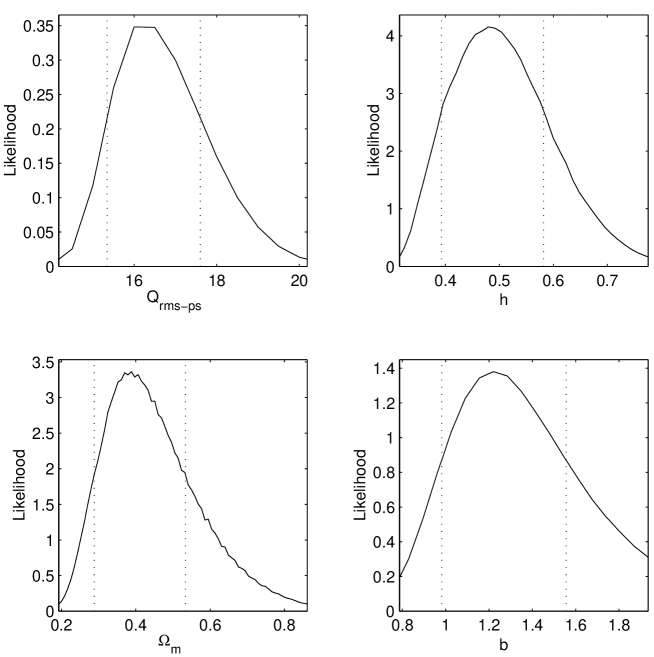
Figure 5: The one-dimensional marginalised probability distributions for each of the four parameters. The vertical dashed lines denote the 68% confidence limits. The horizontal plot limits are at the 99% confidence limits.

To obtain 68 per cent confidence limits on each of the free parameters it is necessary to marginalise over the remaining free parameters. To achieve this we evaluated the joint likelihood function on a 4-dimensional grid of parameter values. The range of values and number of grid points in each direction were $5<Q<30$, $50$ steps; $0.3<{h}<0.9$, $50$ steps; $0.1<{\Omega_{\rm m}}<1.0$, $100$ steps; $0.7<{b_{\rm iras}}<2.0$, $20$ steps. For each parameter, the corresponding one-dimensional marginalised probability distribution was calculated by integrating the likelihood function over the other variables. The marginalised distribution for each parameter is shown in Fig. 5, in which the dashed vertical lines denote the 68% confidence limits quoted in Table 1. In general, the peak of the one-dimensional probability distribution for each variable will differ from the global optimum across all parameters. However, for all four variables in this system, the two values are found to be extremely close.

In addition we evaluated the covariance matrix at the joint optimum. The covariance matrix is simply the inverse of the Hessian at the joint optimum. The Hessian is given by ${{\partial^{2}{\rm ln}\left({\cal L}_{\rm joint}\right)}/({\partial\alpha_{i}\partial\alpha_{j}})}$ for pairs of parameters $\alpha_{i}$ and $\alpha_{j}$ and is evaluated using a standard central-difference algorithm. Taking the square-root of the diagonal elements of the covariance matrix, the standard errors on the parameters are found to be $\Delta Q=0.67$ $\mu$K, $\Delta{h}=0.03$, $\Delta{\Omega_{\rm m}}=0.04$ and $\Delta{b_{\rm iras}}=0.1$. Comparing these with the marginalised errors quoted in Table 1 we note that the marginalised errors are consistently larger, as expected. By rescaling the covariance matrix so that its diagonal elements equal unity, we obtain the correlation matrix shown in Table 2. We see that the most strongly correlated parameters are ${\Omega_{\rm m}}$ and $h$.

	$Q$	${h}$	${\Omega_{\rm m}}$	${b_{\rm iras}}$
$Q$	$1.00$	$0.40$	$-0.46$	$-0.49$
${h}$	$0.40$	$1.00$	$-0.82$	$-0.57$
${\Omega_{\rm m}}$	$-0.46$	$-0.82$	$1.00$	$0.09$
${b_{\rm iras}}$	$-0.49$	$-0.57$	$0.09$	$1.00$

Table 2: Parameter correlation matrix at the joint optimum

6 Discussion

The results of this joint optimisation are in reasonable agreement with other current estimates. The relatively low value of ${\Omega_{\rm m}}\approx 0.4$ is close to that found by others (White et al. (1993); Bahcall, Fan and Cen (1997)), and is in line with recent supernovae results (Perlmutter et al. (1998)). However, given the assumption of a flat universe, it requires a very high cosmological constant (${\Omega_{\Lambda}}=0.6$). Gravitational lensing measurements have constrained ${\Omega_{\Lambda}}<0.7$ (Kochanek (1996), Falco, Kochanek & Munoz (1998)). Our value for the Hubble constant, ${h}=0.53$, agrees well with several other measurements (Sugiyama (1995); Lineweaver et al. (1997)), but falls at the low end of the generally accepted range from local measurements (Freedman et al. (1994)). Assuming the nucleosynthesis constraint $\Omega_{b}h^{2}=0.024$ (Tytler, Fan & Burles (1996), Steigman, Hata & Felten (1998)), the optimal baryon density is found to be ${\Omega_{\rm b}}=0.085$. Our value for the combination ${\sigma_{8}}{\Omega_{\rm m}}^{0.6}=0.38$ is lower than the one derived from measurements from the peculiar velocity field, $\sigma_{8}{\Omega_{\rm m}}^{0.6}\approx 0.8$ (Freudling et al. (1998)). Our values are closer to the combination derived from cluster abundance $\sigma_{8}{\Omega_{\rm m}}^{0.5}\approx 0.5$ (Eke, Cole & Frenk (1996), Bahcall, Fan and Cen (1997)). Finally, for spatially-flat universes the time since the Big Bang for the values of our ${\Omega_{\rm m}}$ and $h$ at the joint optimum is $16.5$ Gyr.

On the IRAS side, ${\beta_{\rm iras}}=0.47$ is in agreement with several other measurements (Strauss (1989); Schlegel (1995); Willick et al. (1997)), although there are other measurements which place ${\beta_{\rm iras}}$ much higher (Dekel et al. (1993); Sigad et al. (1998)). Willick et al. (1997) discuss the discrepancies between the various measurement techniques, and why they lead to such distinct results. Finally, the IRAS mass-to-light bias is seen to be slightly greater than unity (${b_{\rm iras}}=1.21$), suggesting that the IRAS galaxies (mainly spirals) are reasonable (but not perfect) tracers of the underlying mass distribution. We also note that our joint IRAS+CMB optimal values for $\sigma_{8,{\rm iras}},\beta_{{\rm iras}}$ and $\Gamma$ (Table 1) are in perfect agreement with the values derived from IRAS alone (FSL, Fisher (1994)). However at fixed $\sigma_{8,{\rm iras}}=0.69$ based on the IRAS correlation function FSL found a higher $\beta_{{\rm iras}}=0.94\pm 0.17$ and $\Gamma=0.17\pm 0.05(1-\sigma)$. We emphasise that the naive linear biasing should be generalised to more realistic scenarios (e.g. Dekel and Lahav (1998)).

As discussed in Section 5, the total CMB+IRAS reduced $\chi^{2}$ at the joint optimum is 1.16, indicating that the optimum model is a good fit to both data-sets. We may compare this value with that obtained by Gawiser & Silk (1998). Using several data-sets Gawiser & Silk (1998) found the reduced $\chi^{2}$ for $\Lambda$CDM to be 1.9, as opposed to a value of 1.2 for their ‘best’ model of Cold+Hot Dark matter (CHDM). However, using only the CMB and IRAS $\chi^{2}$ values for $\Lambda$CDM in their Table 3, the total reduced $\chi^{2}$ is found to be 1.00 as compared to a value of 0.95 for CHDM. Thus, using only the CMB and IRAS data-sets, $\Lambda$CDM is found to fit the observations as well as CHDM, and the results quoted by Gawiser & Silk (1998) are consistent with those presented here.

The near future will see a dramatic increase in LSS data (e.g. the PSCZ, SDSS, 2dF surveys) and detailed measurements of the CMB fluctuations on sub-degree scales (e.g. from the Planck Surveyor and MAP satellites). These will allow more accurate parameter estimation and the untying of the various parameters held fixed in the present work.

Acknowledgments

We would like to thank E. Gawiser, J. Felten, J. Silk, G. Steigman, K. Wu and I. Zehavi for helpful discussions. Matthew Webster and Sarah Bridle acknowledge PPARC studentships. Graça Rocha acknowledges a NSF grant EPS-9550487 with matching support from the State of Kansas and from a K*STAR First award.

Figure 1: The data points used in the calculation of the CMB likelihood function. The overlaid curve is a model evaluated with optimal parameters shown in Table 1.

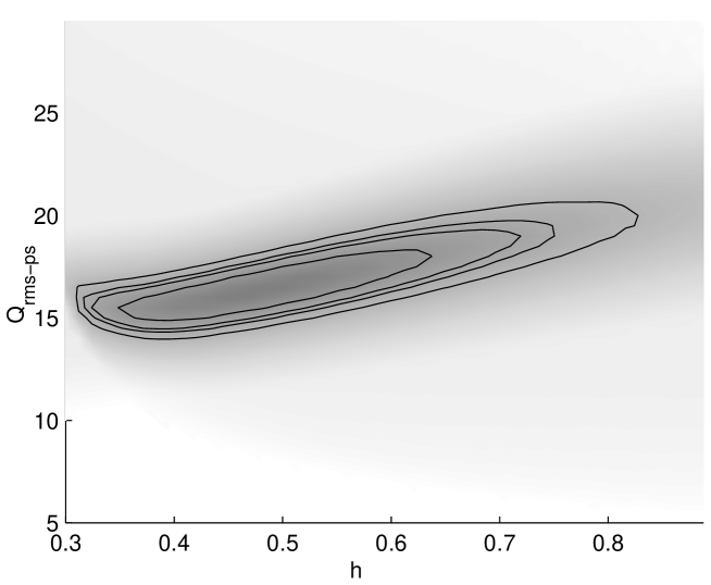
Figure 4: The joint CMB+IRAS likelihood function in the {${h}$, $Q$}-plane after marginalisation over ${\Omega_{\rm m}}$ and ${b_{\rm iras}}$. The contours denote the 68, 90, 95 and 99 per cent confidence regions.

References

- Bagla (1998) Bagla, J., S., 1998, MNRAS, in press, astro-ph/9711081)
- Bahcall, Fan and Cen (1997) Bahcall N.A., Fan, X., & Cen, R. 1997, ApJ, 485, L53
- Baker et al. (1998) Baker J.C. et al. , 1998, MNRAS, submitted
- Bardeen et al. (1986) Bardeen J.M., Bond J.R., Kaiser N. & Szalay A.S., 1986, ApJ, 304, 15
- Bennett et al. (1996) Bennett C.L. et al. , 1996, ApJ., 464, L1
- Blanton et al. (1998) Blanton, M., Cen, R., Ostriker, J.P., & Strauss, M.A., 1998, astro-ph/9807029
- (7) Bond J.R., 1995, Cosmology and Large Scale Structure ed. Schaeffer, R. Elsevier Science Publishers, Netherlands, Proc. Les Houches School, Session LX, August 1993
- (8) Bond J.R., 1995, Astrophys. Lett. and Comm., 32, 63
- (9) Bond J.R., Davis R.L. & Steinhardt P.J., 1995, Astrophys. Lett. and Comm., 32, 53
- Carroll, Press & Turner (1992) Carroll S.M., Press W.H. & Turner E.L., 1992, Ann. Rev. Astron. & Astrophy., 30, 499
- Cheng et al. (1994) Cheng E.S. et al. , 1994, ApJ., 422, L37
- Cheng et al. (1996) Cheng E.S. et al. , 1996, ApJ., 456, L71
- Cole et al. (1995) Cole S., Fisher K.B. & Weinberg D.H., 1995, MNRAS, 275, 515
- De Bernardis et al. (1994) De Bernardis P. et al. , 1994, ApJ., 422, L33
- Dekel et al. (1993) Dekel A., Bertschinger E., Yahil A., Strauss M., Davis M. & Huchra J., 1993, ApJ, 412, 1
- Dekel and Lahav (1998) Dekel, A. & Lahav, O., submitted to ApJ, astro-ph/9806193
- Efstathiou, Bond & White (1995) Efstathiou G., Bond J.R. & White S.D.M., 1992, MNRAS, 258, P1
- Eisenstein, Hu & Tegmark (1998) Eisenstein, D.J., Hu, W. & Tegmark, M., 1998, astro-ph/9807130
- Eke, Cole & Frenk (1996) Eke, V.R., Cole, S., and Frenk, C.S., 1996, MNRAS, 282, 263
- Falco, Kochanek & Munoz (1998) Falco, E.E, Kochanek, C.S. & Munoz, J.A., 1998, ApJ, 494, 47
- Fisher (1994) Fisher, K.B., in proceedings of ‘Cosmic Velocity Fields’, Paris, eds. Bouchet et al., pg. 177, Editions Frontieres
- Fisher, Scharf & Lahav (1994) Fisher, K.B., Scharf, C.A. & Lahav, O., 1994, MNRAS, 266, 219
- Fisher et al. (1995) Fisher, K.B., Huchra, J.P., Strauss, M.A., Davis, M., Yahil A., Schlegel D., 1995, ApJ, 100, 69
- Fisher & Nusser (1996) Fisher K.B. & Nusser A., 1996, MNRAS, 279, L1
- Freedman et al. (1994) Freedman W., et al. , 1994, Nature, 371, 757
- Freudling et al. (1998) Freudling et al., 1998, submitted to ApJ
- Gawiser & Silk (1998) Gawiser E., & Silk J., 1998, Science, 280, 1405
- Gundersen et al. (1995) Gundersen J.O et al. , 1995, ApJ., 443, L57
- Gutierrez (1997) Gutierrez C.M., 1997, ApJ., 483, 51
- Hancock et al. (1994) Hancock S., et al. , 1994, Nature, 367, 333
- Hancock et al. (1997) Hancock S., Gutierrez C.M., Davies R.D., Lasenby A.N., Rocha G., Rebolo R., Watson R.A., Tegmark M., 1997, MNRAS, 298, 505
- Hancock et al. (1998) Hancock S., Rocha G., Lasenby A.N., Gutierrez C.M., 1998, MNRAS, 294, L1
- Heavens & Taylor (1995) Heavens A.F. & Taylor A.N., 1995, MNRAS, 275, 483
- Kaiser (1987) Kaiser N., 1987, MNRAS, 227, 1
- Kaiser et al. (1991) Kaiser N., Efstathiou G., Ellis R., Frenk C., Lawrence A., Rowan-Robinson M., Saunders W., 1991, MNRAS, 252, 1
- Kochanek (1996) Kochanek C.S., 1996, ApJ, 466, 638
- Lahav et al. (1994) Lahav, O., Fisher, K.B., Hoffman, Y., Scharf, C.A, & Zaroubi, S., 1994, ApJL, 423, L93
- Lahav (1996) Lahav O., 1996, Helv. Phys. Acta, 69, 388
- Leitch et al. (1998) Leitch E.M., Readhead A.C.S., Pearson T.J., Myers S.T., & Gulkis S., 1998, astro-ph/9807312
- Lineweaver et al. (1997) Lineweaver C.H., Barbosa D., Blanchard A. & Bartlett J.G., 1997, Astron. & Astrophy., 322, 365
- Netterfield et al. (1997) Netterfield C.B., Devlin M.J., Jarosik N., Page L., Wollack E.J., 1997, ApJ, 474, 47
- Peebles (1980) Peebles, P.J.E., 1980, The Large-Scale Structure of the Universe, (Princeton: Princeton University Press)
- Pen (1998) Pen, U.-L., 1998, astro-ph/9711180
- Perlmutter et al. (1998) Perlmutter S., et al. , 1998, Nature, 391, 51
- Platt et al. (1997) Platt S.R., Kovac J., Dragovan M., Peterson J.B., & Ruhl J.E., 1997, ApJ, 475, L1
- Press et al. (1992) Press, W.H., Teukolsky, S.A., Vetterling, W.T., & Flannery, B.P., 1992, Numerical Recipes (Second Edition) (Cambridge: Cambridge University Press)
- Rocha et al. (1998) Rocha, G., Hancock, S., Lasenby, A.N., & Gutierrez, C.M. in preparation.
- Ruhl et al. (1995) Ruhl J.E., Dragovan M., Platt S.R., Kovac J., & Novak G., 1995, ApJ., 453, L1
- Scaramela & Vittorio (1990) Scaramela N., & Vittorio N., 1990, ApJ., 353, 372
- Scaramela & Vittorio (1993) Scaramela N., & Vittorio N., 1993, ApJ., 411, 1
- Schlegel (1995) Schlegel D., 1995, Ph. D. Thesis, University of California, Berkeley
- Scott, Srednicki and White (1994) Scott D., Srednicki M., & White M., 1994, ApJ., 241, L5
- Scott et al. (1996) Scott, P.F. et al. , 1996, ApJ., 461, L1
- Seljak & Zaldarriaga (1996) Seljak U., & Zaldarriaga M., 1996, ApJ, 469, 437
- Sigad et al. (1998) Sigad Y., Dekel A., Strauss M.A. & Yahil A., 1998, 495, 516
- Smoot et al. (1992) Smoot, G.F. et al. , 1992, ApJ., 396, L1
- Steigman, Hata & Felten (1998) Steigman, G., Hata, N. & Felten, J.E., 1998, astro-ph/9708016
- Strauss (1989) Strauss M.A., Ph. D. Thesis, University of California, Berkeley
- Strauss & Willick (1995) Strauss, M.A., & Willick, J.A., 1995, Phys Rev, 261, 271
- Sugiyama (1995) Sugiyama N., 1995, ApJ Supp., 100, 281
- Tanaka et al. (1996) Tanaka, S.T. et al. , ApJ, 468, L81
- Tegmark & Peebles (1998) Tegmark, M., & Peebles, P.J.E. 1998, astro-ph/9804067
- Tytler, Fan & Burles (1996) Tytler D., Fan X.M. & Burles S., 1996, Nature, 381, 207
- White et al. (1993) White et al. , 1993, Nature, 366, 429
- Willick et al. (1997) Willick J.A., Strauss M.A., Dekel A. & Kolatt T., 1997, ApJ, 486, 629
- Yahil et al. (1991) Yahil, A., Strauss, M.A., Davis, M., & Huchra, J.P., 1991, ApJ, 372, 380