Hydrodynamics and stability of galactic cooling flows

Abstract

Using numerical techniques we studied the global stability of cooling flows in giant elliptical galaxies. As an initial equilibrium state we choose the hydrostatic gas recycling model [Kritsuk 1996]. Non-equilibrium radiative cooling, stellar mass loss, heating by type Ia supernovae, distributed mass deposition, and thermal conductivity are included. Although the recycling model reproduces the basic X-ray observables, it appears to be unstable with respect to the development of inflow or outflow. In spherically symmetry the inflows are subject to a central cooling catastrophe, while the outflows saturate in a form of a subsonic galactic wind. Two-dimensional axisymmetric random velocity perturbations of the equilibrium model trigger the onset of a cooling catastrophe, which develops in an essentially non-spherical way. The simulations show a patchy pattern of mass deposition and the formation of hollow gas jets, which penetrate through the outflow down to the galaxy core. The X-ray observables of such a hybrid gas flow mimic those of the equilibrium recycling model, but the gas temperature exhibits a central depression. The mass deposition rate $\dot{M}$ consists of two contributions of similar size: (i) a hydrostatic one resembling that of the equilibrium model, and (ii) a dynamical one which is related to the jets and is more concentrated to the centre. For a model galaxy, like NGC 4472, our 2D simulations predict $\dot{M}\approx 2$ M_⊙ yr^-1 within the cooling radius for the advanced non-linear stage of the instability. We discuss the implications of these results to H$\alpha$ nebulae and star formation in cooling flow galaxies and emphasize the need for high-resolution 3D simulations.

1 Introduction

X-ray observations of normal early-type galaxies with the Einstein observatory have revealed an extended diffuse thermal emission from the hot (0.5-2 keV) component of their interstellar medium [ISM] [Forman et al. 1979]. With luminosities $L_{\mathrm{X}}\sim 10^{39}$-$10^{42}$ erg s^-1 this hot gas contributes $10^{9}-10^{10}$ M_⊙ to the total galaxy mass in its optical confines (Forman, Jones & Tucker 1985). The X-ray luminosities correlate with the optical (blue) luminosities of early-type galaxies, although with a large spread of $L_{\mathrm{X}}$ at a fixed $L_{\mathrm{B}}$ [Canizares, Fabbiano & Trinchieri [Canizares et al. 1987]; Donnelly, Faber & O’Connell [Donnelly et al. 1990]; Eskridge, Fabbiano & Kim [Eskridge et al. 1995]]. For nearby bright ellipticals the surface brightness distributions in X-rays and in the optical are similar as far as the interaction of the galaxy X-ray emitting gas with the surrounding medium is unimportant (Trinchieri, Fabbiano & Canizares 1986). ROSAT observations revealed correlations of the temperature of the hot gas with the stellar velocity dispersion and with the abundances for a complete sample of 43 elliptical galaxies [Davis & White 1996]. Galaxies with higher velocity dispersions tend to have higher, approximately solar, abundances and higher diffuse gas temperatures. In all cases the gas is substantially (a factor of $\sim 2$) hotter than the kinetic temperature of the luminous stars indicating the presence of dark haloes. The analysis of spectral properties for a sample of 12 early-type galaxies observed with ASCA has revealed systematically lower abundances with a mean value of about 0.3 solar and has confirmed the relationship between stellar velocity dispersion and gas temperature [Matsumoto et al. 1997]. Gas temperature profiles for elliptical galaxies determined with ROSAT and ASCA have been found to be surprisingly uniform for projected radii $r\leq 10\>r_{\mathrm{e}}$ ($r_{\mathrm{e}}$ is the so-called effective or half-light radius). They exhibit a positive temperature gradient out to $\sim 3\>r_{\mathrm{e}}$ followed by a leveling off or gradual decrease toward larger radii [Brighenti & Mathews 1997]. In addition to hot X-ray emitting gas early-type galaxies have been shown to have a cooler component ($10^{7}-10^{8}$ M_⊙) detectable at 100 $\mu$m [Jura et al. 1987] as well as warm ionized gas ($10^{3}-10^{5}$ M_⊙ in the central 1-10 kpc) producing optical emission lines [Caldwell 1984, Demoulin-Ulrich et al. 1984, Phillips et al. 1986, Buson et al. 1993, Singh et al. 1995, Macchetto et al. 1996].

Initially, steady-state cooling flow models were invoked to interpret X-ray observations [Thomas et al. 1986, Sarazin & White 1987, Sarazin & White 1988, Vedder et al. 1988, Sarazin & Ashe 1989]. This, in essence, empirical approach was based on the simple idea that if the cooling time-scale is shorter than the Hubble time near the centre, but still longer than the gravitational time-scale, then a very subsonic quasi-hydrostatic inflow must take place. However, the global stability of these early models has not been proved yet. Later time-dependent hydrodynamic modeling has demonstrated that, in general, such accretion flows are unstable and suffer cooling catastrophes at their centres, which were difficult to reconcile with observations [Meiksin 1988, Murray & Balbus 1992]. Secular variations of the stellar mass-loss rate and supernova heating rate due to stellar evolution in the galaxy allowed for a description of the evolution of the hot ISM in ellipticals on the Hubble time-scale [D’Ercole et al. [D’Ercole et al. 1989]; Ciotti et al. [Ciotti et al. 1991]; David, Forman & Jones (1990, 1991) ]. The resulting models evolved through up to three consecutive evolutionary stages: the wind, outflow and inflow phases. Accordingly, most of present-day ellipticals are in the outflow phase, while a few of the brightest galaxies may have already experienced their transition to the inflow regime. Although the problem of the cooling catastrophe was not resolved, an important outcome of spherically symmetric evolutionary modeling was the understanding that the use of steady-state cooling flow models to diagnose mass accretion rates in dynamical situations can lead to erroneous results [Ciotti et al. 1991, Murray & Balbus 1992].

In the absence of direct measurements of the flow velocity a systematic study of global hydrodynamic and thermal stability properties of the hot ISM in ellipticals can provide a selection criterion for realistic flow regimes. Starting from the essential physics of cooling flows, we have constructed a hydrostatic equilibrium model, which describes a stable in situ recycling of gas shed by stars through local thermal instabilities into a condensate, which can become the material for further star formation [Kritsuk 1996].

In this paper we probe the global stability of the recycling model in the inflow-outflow context. Section 2 describes the basic assumptions of the hot ISM model and of the underlying galaxy model. Section 3 gives the details of the numerical method used in the simulations. The evolution of spherically symmetric perturbations and their stabilization by a conductive heat flux are considered in Section 4. In Section 5 we abandon the restrictive assumption of spherical symmetry and study the development of instabilities by means of two-dimensional simulations. This allows for a better insight into the complex physics of cooling flows. The discussion and conclusions can be found in Sections 6 and 7, respectively.

2 The model

2.1 Input physics

It is usually assumed that the source of the hot ISM in elliptical galaxies is provided mainly by mass loss in the form of winds from red giant stars orbiting in the gravitational potential of the stellar system and its dark halo. The gas is supposed to be well mixed by ‘collisions’ of the winds originating from stars, which pass by close to each other.

Supernova (SN) explosions of type Ia are considered to be a major potential heating source for the gas, although there is a great uncertainty in the rate of SNe Ia. SNe can also play an important role in the gas enrichment with heavy elements, if the ejecta are well mixed with the ISM before they cool down considerably.

We assume that evolutionary processes in the stellar system provide a steady source of small-scale non-linear perturbations, which unavoidably become thermally unstable in the temperature regime of interest. Heat conduction, which is efficient in such a hot tenuous plasma, is able to suppress the growth of small-amplitude perturbations in the short wavelength limit. However, because of different non-linear dependencies of the conduction flux and the radiative cooling rate on local physical conditions in the gas, finite amplitude small-scale perturbations will still be able to grow non-linear. Hence, a fraction of the gas will quasi-isobarically cool down to at least $T\sim 10^{4}$ K (becoming $\geq 10^{3}$ times denser) and will drop out from the flow, thereby enhancing the overall cooling of the gas and removing a fraction of its momentum.

The final fate of the condensing material is still a matter of debate. If at some later point star formation occurs in the cold condensate, one can expect that feedback heating by SNe II and Ib/c will return part of the energy back to the hot phase (with some delay). Currently our simplified model does not incorporate this feedback heating.

Thus, we introduce a set of sources of mass, momentum and energy of the hot ISM, which are distributed over the whole galaxy. Their efficiencies depend both on the local physical conditions in the gas and on the local parameters of the stellar system. It is one of the purposes of our hydrodynamic modeling to follow the evolution of a hot corona driven by the competition between sources and sinks. In several other evolutionary calculations the rates of processes directly related to stellar evolution (e.g., the SN rate) were assumed to be variable on a time scale of a few Gyr. However, we keep the rates constant and concentrate mainly on the short-term evolution of the cooling flows excluding the early phases of galaxy formation from our consideration.

Our hydrodynamic description is valid only on scales $l\geq{\cal L}=\max\{l^{\mathrm{wn}},l^{\mathrm{sn}},l^{\mathrm{ti}}\}$, which are larger than the maximum scale associated with discrete physical sources, such as a region blown by a stellar wind ($l^{\mathrm{wn}}$), a SN remnant ($l^{\mathrm{sn}}$), or a cooling condensation ($l^{\mathrm{ti}}$). The scale ${\cal L}$ depends on the distance from the galactic centre. We refer to [Mathews 1990] for a detailed discussion of these issues [see also [Kritsuk 1992] for details on thermal instabilities].

Below we briefly define the parameters, which control the efficiency of the sources.

2.1.1 Stellar mass loss

The rate of gas supply to the ISM due to stellar mass loss and SNe Ia is defined as $\alpha\rho_{*}(r)$, where $\rho_{*}$ is the stellar mass density and $\alpha=\alpha_{*}+\alpha_{\mathrm{sn}}\equiv const$. It incorporates a contribution from ‘quiescent’ stellar mass loss $\alpha_{*}\simeq 4.7\times 10^{-20}$ s^-1 [Faber & Gallagher 1976, Sarazin & White 1987] with a small addition by supernovae $\alpha_{\mathrm{sn}}=3.1\times 10^{-21}$ s^-1 (the estimate corresponds to $r_{\mathrm{sn}}=0.55\>h_{75}^{2}$ SNu, $M_{\mathrm{sn}}=1.4\;M_{\odot}$, and $(M/L_{B})_{*}=8\;M_{\odot}/L_{\odot}$). According to van den Bergh & Tammann [van den Bergh & Tammann 1991] the SNe Ia rate, $r_{\mathrm{sn}}$, is uncertain by a factor of the order of 1.5, but a significantly lower estimate for E/S0 galaxies, $r_{\mathrm{sn}}=0.15\pm 0.06\>h_{75}^{2}$, was derived by Cappellaro et al. [Cappellaro et al. 1997].

2.1.2 Radiative cooling

We use a non-equilibrium radiative cooling function $\Lambda(T,Z_{\odot})$ erg cm³g^-2s^-1 for optically thin hot plasma, defined in the temperature range $T\in[10^{4},10^{8.5}]$ K, which we compiled from [Sutherland & Dopita 1993] for the case of a solar gas metallicity $Z_{\odot}$, zero diffuse radiation field, and with abundance ratios taken from [Anders & Grevesse 1989].

2.1.3 Mass deposition

We define the rate of mass deposition to be a function of the local conditions in the hot ISM, $\dot{\rho}_{\mathrm{ti}}=b\chi(n)\rho$, where $\rho$ is the gas mass density. The spectrum of primeval small-scale perturbations in the gas and, in particular, its deformation by heat conduction are described by a parameter $b\equiv const\in[0,\;1]$. The Heaviside function $\chi$ and the linear instability growth rate $n$ are defined as

$$\chi(n)=\cases{n,&if $n\geq 0$;\cr 0,&otherwise;}$$ (1)

$$n\equiv{\partial\over\partial t}\left(\ln{\delta\rho\over\rho}\right)={1\over c_{p}}\left({2\rho\Lambda\over T}-\rho{\mathrm{d}\Lambda\over\mathrm{d}T}\right)-{\alpha\rho_{*}\over\rho}.$$ (2)

Here $c_{p}$ is the specific heat at constant pressure. The first term in the rhs of equation (2) coincides with Field’s instability criterion, the second one describes stabilization due to stellar mass loss [Kritsuk 1992]. We assume $b=0.5$ for the models described in this paper. The motivation for this choice can be found in [Kritsuk 1996].

2.1.4 Distributed heating

The rate of heating due to thermalization of stellar winds and due to SNe Ia is assumed to be equal to $\alpha\rho_{*}T_{0}$, where $T_{0}=(\alpha_{*}T_{*}+\alpha_{\mathrm{sn}}T_{\mathrm{sn}})/\alpha$ is the characteristic temperature of the heat source. Heating by thermalization of winds from stars orbiting in the galactic potential is defined by $T_{*}={\mu\sigma_{*}^{2}\over{\cal R}}=6.47\times 10^{6}$ K (we assume $\sigma_{*}=300$ km/s and a mean molecular weight $\mu=0.63$; ${\cal R}$ is the gas constant). The SN temperature $T_{\mathrm{sn}}={\mu v_{\mathrm{ej}}^{2}\over 3{\cal R}}=1.09\times 10^{9}$ K for $E_{\mathrm{sn}}=6\times 10^{50}$ erg and $M_{\mathrm{sn}}=1.4\;M_{\odot}$. With these values $T_{0}\simeq 7\times 10^{7}$ K, while for $r_{\mathrm{sn}}=0.15$ SNu the source temperature is lower: $T_{0}\simeq 2.6\times 10^{7}$ K. We assume $T_{0}=5\times 10^{7}$ K in our simulations.

2.1.5 Thermal conduction

The large-scale heat flux $q$$=-\eta\cdot\kappa\nabla T$ is defined through a reduction factor $\eta\leq 1$, which is treated as a free parameter, and the Spitzer [Spitzer 1962] conductivity coefficient for a fully ionized gas

$$\kappa={1.84\times 10^{-5}T_{\mathrm{e}}^{5/2}\over\ln{\Lambda_{\mathrm{c}}}}\;\;\mathrm{ergs\;s^{-1}\;K^{-1}\;cm^{-1}},$$ (3)

where for $T>4.2\times 10^{5}$ K the Coulomb logarithm is $\ln{\Lambda_{\mathrm{c}}}=32.0+\ln{[n^{-1/2}(T_{\mathrm{e}}/10^{7}}$ K)].

2.2 ‘Thermodynamic’ equilibrium

The combination of distributed sources presented above allows stable steady-state solutions, which were analyzed in the framework of a ’closed-box’ model [Kritsuk 1996]. These solutions describe the ISM in ‘thermodynamic’ equilibrium, i.e. in a state, where the sources and sinks of mass and energy are locally balanced.

An equilibrium temperature of one such state, calculated for our assumed set of parameter values, is $T_{\mathrm{eq}}(\alpha,b,T_{0},Z)\approx 1.4\times 10^{7}$ K. This temperature is close to the temperature estimates for hot gaseous coronae based upon the X-ray data of nearby giant ellipticals.

The characteristic time scale, on which the gas is able to reach thermodynamic equilibrium from any point in the huge attraction region of the phase plane $(\rho,T)$,

$$t_{\mathrm{s}}=\sqrt{t_{\mathrm{c}}t_{\alpha}},$$ (4)

is the geometric mean of the local cooling time $t_{\mathrm{c}}\equiv c^{2}/[(\gamma-1)\rho\Lambda]$ and the time scale for stellar mass loss $t_{\alpha}=(\alpha\rho_{*}/\rho)^{-1}$; $c$ is the isothermal sound speed, and $\gamma={5\over 3}$ is the ratio of specific heats.

2.3 Hydrostatic equilibrium

For simplicity we assume that the source parameters $\alpha$, $b$, $T_{0}$, and $Z$ do not depend on radius. This implies that the equilibrium temperature $T_{\mathrm{eq}}$ is also radius independent. Hence, if the gas is in thermodynamic equilibrium, it can hydrostatically fill only the potential well of an isothermal sphere. It is known, however, that due to dissipation the shapes of density profiles of stars and dark matter usually do not coincide in giant galaxies. We therefore choose a potential of a two-component isothermal sphere, which incorporates stars and dark matter with different velocity dispersions [Kritsuk 1996, Kritsuk 1997a]. We define the parameter $\beta$ as a ratio of these dispersions,

$$\beta\equiv{\sigma_{*}^{2}\over\sigma_{\mathrm{DM}}^{2}}<1.$$ (5)

This two-component model is completely defined by four parameters. Once, we fix $\sigma_{\mathrm{DM}}^{2}={{\cal R}\over\mu}T_{\mathrm{eq}}$ (since hot gas and dark matter are usually distributed similarly) and $\beta$=0.5 [see [Kritsuk 1996] for details], we have to define only two additional quantities, namely, the characteristic radius of the gravitating matter distribution

$$r_{0}=\frac{\sigma_{*}}{\sqrt{4\pi G\rho_{*,0}}},$$ (6)

and the ratio of dark matter density to stellar density at the centre

$$\delta=\rho_{\mathrm{DM},0}/\rho_{*,0}.$$ (7)

We set $\delta=10^{-1.5}$, since the stellar component dominates by mass in the central regions of giant ellipticals. Such a choice of $\beta$ and $\delta$, which control the shape of the density distributions [Kritsuk 1997b], corresponds to a galaxy, whose surface brightness profile follows the de Vaucouleurs law, and which contains comparable amounts of mass in luminous and dark matter within its effective radius. Finally, in order to fix the scaling of physical values, we set the characteristic radius $r_{0}=0.16$ kpc. This particular choice of parameters allows us to reproduce with reasonable accuracy the shape of the surface brightness profile for NGC 4472 (M49), the optically most luminous E2 galaxy in the Virgo cluster, assuming a distance of 17 Mpc [Trinchieri et al. 1986].

Numerical integration of the Poisson and Jeans equations for the given set of parameters provides us with a giant spheroidal model galaxy with a total mass in stars $M_{*}\approx 8.5\times 10^{11}$ M_⊙ and a stellar velocity dispersion $\sigma_{*}\approx 304$ km s^-1.

The hydrostatic isothermal gas distribution in its gravitational potential follows the so-called $\beta$-law: $\rho_{\mathrm{eq}}\propto\rho_{*}^{\beta}$ with $\beta=0.5$. This implies that, as it is observed, the shapes of the optical and the X-ray brightness profiles are identical [cf. [Trinchieri et al. 1986]] and $T_{\mathrm{eq}}=2T_{*}$ [cf. [Davis & White 1996]]. The self-gravity of the ISM is negligible and is not taken into account.

The central equilibrium gas density is $\rho_{\mathrm{eq,0}}/(\mu m_{\mathrm{H}})\approx 0.19$ cm^-3 and the time scale associated with the sources at the centre is $t_{\mathrm{s,0}}\approx 4.9\times 10^{7}$ yr. The gravitational time scale

$$t_{\mathrm{G}}={1\over\sqrt{4\pi G\rho_{*,0}}}={r_{0}\over\sigma_{*}}\approx 2.1\times 10^{6}\;\mathrm{yr}$$ (8)

is much shorter than $t_{\mathrm{s,0}}$. The cooling radius, fixed at the distance where $t_{\mathrm{c}}=10$ Gyr, is $r_{\mathrm{cool}}=36$ kpc.

2.4 Basic equations

We probe the global stability of the equilibrium hydrostatic gas configuration with respect to a variety of perturbations by means of numerical solutions of the time-dependent hydrodynamic equations for the mass, momentum and energy balance in the hot ISM:

$$\frac{\partial\rho}{\partial t}+\nabla\cdot(\rho\mn@boldsymbol{v})=\alpha\rho_{*}-\dot{\rho}_{\mathrm{ti}},$$ (9)

$$\frac{\partial(\rho\mn@boldsymbol{v})}{\partial t}+\nabla(\rho\mn@boldsymbol{v}^{2}+p)=\rho\nabla\phi-\dot{\rho}_{\mathrm{ti}}\mn@boldsymbol{v},$$ (10)

$$\frac{\partial E}{\partial t}+\nabla\cdot[\mn@boldsymbol{v}(E+p)]=$$ (11)

$$\alpha\rho_{*}e_{*}-\dot{\rho}_{\mathrm{ti}}(E+p)/\rho-\rho^{2}\Lambda+\rho\mn@boldsymbol{v}\cdot\nabla\phi-\nabla\cdot\mn@boldsymbol{q}.$$

Here $\mn@boldsymbol{v}$ is the velocity, $p=(\gamma-1)e\rho$ is the pressure, $e$ is the specific internal energy, $e_{*}=c_{\mathrm{v}}T_{0}$, and the energy density $E=\rho(e+\mn@boldsymbol{v}^{2}/2)$.

2.5 Initial conditions

The undisturbed state is considered to be a spherically symmetric gas configuration in hydrostatic and thermodynamic equilibrium:

$$\left.\rho\right|_{t=0} = \rho_{\mathrm{eq}}(r),$$ (12)

$$\left.p\right|_{t=0} = p_{\mathrm{eq}}(r)\equiv{{\cal R}\over\mu}\rho_{\mathrm{eq}}T_{\mathrm{eq}},$$ (13)

$$\left.\mn@boldsymbol{v}\right|_{t=0} = 0.$$ (14)

For one-dimensional spherically symmetric simulations we introduce a global density perturbation with an amplitude $\epsilon=const$:

$$\left.\rho\right|_{t=0}=(1+\epsilon)\rho_{\mathrm{eq}}(r).$$ (15)

For the 2D axisymmetric simulations, which were performed in spherical coordinates $(r,\vartheta,\varphi)$, we used either a single-wave isothermal density perturbation of the form

$$\left.\rho\right|_{t=0}=\left[1+\epsilon\left(\cos^{2}{\vartheta}-0.5\right)\right]\rho_{\mathrm{eq}}(r),$$ (16)

or random large-scale velocity field perturbations, $\mn@boldsymbol{v}=(u,v)$, (where $u$ and $v$ are the radial and the tangential velocity component, respectively) which are defined on the discrete grid (see section 3.3) as follows:

$$\left.u,v\right|_{t=0}=\delta_{u,v}(r,\vartheta),$$ (17)

$$\delta_{a}(r_{k},\vartheta_{l}) = {1\over Q}\sum_{i=1}^{3}\sum_{j=1}^{3}\left(A_{ij}^{a}\cos{2\pi\over n}ik\sin{2\pi\over n}jl+\right.$$

$$B_{ij}^{a}\cos{2\pi\over n}ik\cos{2\pi\over n}jl+$$

$$C_{ij}^{a}\sin{2\pi\over n}ik\sin{2\pi\over n}jl+$$

$$\left.D_{ij}^{a}\sin{2\pi\over n}ik\cos{2\pi\over n}jl\right),$$

with $a\in\{u,v\}$. The computational volume is discretized into $n\times n$ cells, which are labeled by the pair of indices $k,l$. $\{A,B,C,D\}^{a}_{ij}$ are quasi-random numbers from the interval $[-1,\>1]$. The amplitude of the velocity perturbations is normalized by a factor $Q$, so that ${1\over 2}(\max_{k,l}\delta_{a}-\min_{k,l}\delta_{a})=\epsilon$.

We varied the amplitude $\epsilon$ in different experiments in the range from 0.2% to 30%.

2.6 Boundary conditions

We imposed the following conditions on the hydrodynamic variables at the inner spherical boundary at $r_{\mathrm{i}}\approx 0.12\,$kpc:

$$u(r_{\mathrm{i}})=0,\;\;\;\;\;\;\;\;\left.{\partial u\over\partial r}\right|_{r=r_{\mathrm{i}}}=0,$$ (19)

$$v(r_{\mathrm{i}})=0,\;\;\;\;\;\;\;\;\left.{\partial v\over\partial r}\right|_{r=r_{\mathrm{i}}}=0,$$ (20)

$$\left.{\partial T\over\partial r}\right|_{r=r_{\mathrm{i}}}=0,$$ (21)

$$\left.{\partial p\over\partial r}\right|_{r=r_{\mathrm{i}}}=\left.\rho{\nabla\phi}\right|_{r=r_{\mathrm{i}}}.$$ (22)

At the outer spherical boundary at $r_{\mathrm{o}}\approx 151\,$kpc, we used slightly different conditions:

$$u(r_{\mathrm{o}})=0,\;\;\;\;\;\;\;\;\left.{\partial u\over\partial r}\right|_{r=r_{\mathrm{o}}}=0,$$ (23)

$$v(r_{\mathrm{o}})=0,\;\;\;\;\;\;\;\;\left.{\partial v\over\partial r}\right|_{r=r_{\mathrm{o}}}=0,$$ (24)

$$T(r_{\mathrm{o}})=T_{\mathrm{eq}},\;\;\;\;\;\;\;\;\left.{\partial T\over\partial r}\right|_{r=r_{\mathrm{o}}}=0,$$ (25)

$$p(r_{\mathrm{o}})=p_{\mathrm{eq}}(r_{\mathrm{o}}),\;\;\;\;\;\;\;\;\left.{\partial p\over\partial r}\right|_{r=r_{\mathrm{o}}}=\left.\rho{\nabla\phi}\right|_{r=r_{\mathrm{o}}}.$$ (26)

In the 2D axisymmetric calculations we solved the flow equations in a 90 degree sector centered at the equatorial plane and imposed ‘periodic’ boundary conditions in angular direction at $\vartheta_{\mathrm{l,r}}={\pi\over 2}\pm{\pi\over 4}$:

$$a(\vartheta_{\mathrm{l}})=a(\vartheta_{\mathrm{r}}),\;\;\;\;\;\;\;\;\left.{\partial a\over\partial\vartheta}\right|_{\vartheta=\vartheta_{\mathrm{l}}}=\left.{\partial a\over\partial\vartheta}\right|_{\vartheta=\vartheta_{\mathrm{r}}},$$ (27)

where $a\in\{\rho,u,v,p\}$.

3 Numerical method

The numerical solutions discussed in this paper were obtained using the Piecewise Parabolic Method (PPM) [Colella & Woodward 1984] – a second order extension of Godunov’s finite difference scheme, which uses a nonlinear Riemann solver in the hydrodynamic calculations. It was originally described in [Godunov 1959, Godunov et al. 1961] and first adapted for high order difference schemes by van Leer [van Leer 1979]. We use a direct single-step explicit Eulerian formulation of the method for the equations written in conservation form. We solve the equations in spherical coordinates for both spherically symmetric and axisymmetric problems. The coordinate singularities at the centre and along the symmetry axis are isolated by a proper choice of the computational volume and the corresponding boundary conditions (see above).

There are slight differences in our PPM implementation, as compared to the original prescription of Colella & Woodward [Colella & Woodward 1984]. These are stipulated by the presence of source terms, which play an essential role in our modeling.

3.1 Treatment of the source terms

In order to keep the numerical scheme consistent, the expressions for $\beta^{0}$ and $\beta^{\pm}$ [see equation (3.7) of [Colella & Woodward 1984]] have been re-derived to incorporate the terms corresponding to the volume sources of mass, momentum and energy, due to radiative cooling, stellar mass loss, SNe heating and local thermal instabilities. This gives rise to a modification of the procedure for the calculation of the effective left and right states for the Riemann problem. The effect of the source terms on $\overline{U}_{j+1/2}$ is accounted for to second order accuracy. The detailed formulae can be found in [Kritsuk 1998].

The presence of sources, represented by non-linear functions of the hydrodynamic variables, considerably modifies the behaviour of the gas flow. In particular, when the effects of local thermal instabilities are taken into account, the elastic properties of the gas change dramatically. In simple terms, slow gas compression by an external force easily results in condensation of a significant fraction of the gas. The self-accelerating contraction does not meet any considerable resistance by pressure forces, as long as it is slow enough. When simulating such gas flows we observed the formation of ‘condensation fronts’ – thin sheet-like quasi-isobaric structures, characterized by an enhanced density and negative velocity divergence. These fronts, being the major sites of condensation, are able to move in the direction opposite to large-scale pressure gradients and coalesce with each other upon collisions. In order to treat this kind of solutions properly with our numerical scheme, we had to introduce additional dissipation in the vicinity of the fronts. The dissipation algorithm allows us to keep the peak density values finite, limiting the run-away cooling and condensation of the gas in cells located at the front. In fact, we added an explicit diffusive flux to the numerical fluxes in the mass and momentum conservation equations following the simple prescription of Colella & Woodward (1984). Further details of the dissipation algorithm can be found in [Kritsuk 1998]. While we apply the simple flattening around shock fronts [see the Appendix in [Colella & Woodward 1984]] in our 1D calculations, we have switched it off in our 2D simulations.

The sources make the method implicit, since the values of $\rho^{n+1}$ and $\rho^{n+1}u^{n+1}$ depend on $E^{n+1}$ through terms, which include temperature dependent radiative cooling $\Lambda$ and mass deposition $\dot{\rho}_{\mathrm{ti}}$. To avoid an iterative solution method we approximated the unknown values at $t=t^{n+1}$ by those from the previous time level at $t=t^{n}$ in the source terms $\dot{\rho}_{\mathrm{ti}}^{n+1}$ and $\Lambda^{n+1}$, still using the correct treatment elsewhere.

3.2 Introducing the heat flux

In order to estimate the stabilizing effects of thermal conductivity on the isothermal equilibrium solution we include a $\nabla\cdot\boldmath{q}$ term in the final conservative difference step. To keep the scheme explicit, we estimate the temperature values at zone interfaces using the computed left and right state values for pressure and density. Linear approximations of the temperature gradients at the interfaces are computed using the temperature differences in adjacent zones. An adequate reduction of the time step was implemented, too. Such a simplified treatment for the heat conduction flux still allows us to keep the accuracy of the computations sufficiently high in a broad vicinity of the equilibrium solution.

3.3 The computational grid

The computational grid is organized in such a way that it allows us to describe the physically discrete sources as continuously distributed in space. In our particular model the largest scale associated with an individual source is the scale for local thermal instability ($l^{\mathrm{ti}}>l^{\mathrm{sn}}>l^{\mathrm{sw}}$). This scale depends on the degree of suppression of heat conduction by magnetic fields and on the spectrum of the primeval perturbations, which are supplied by ongoing evolutionary processes in the galaxy.

Figure 1: Inflow solution $t=2.4\times 10^{7}$ yr after the start of the simulation for an $\epsilon=10$ % global spherically symmetric density perturbation (solid lines). Dotted lines indicate the unperturbed hydrostatic equilibrium solution. The plots show density, temperature and radial velocity of the gas (left column) together with the surface brightness in X-rays, $I_{\mathrm{x}}$, the mass deposition rate and the efficiency of mass dropout due to thermal instabilities (right column) as functions of the radius. The surface brightness is given in arbitrary units, see text for details.

We introduce a correction factor $\eta$, which defines the scale for growing local thermal instabilities $l^{\mathrm{ti}}\sim 0.3\>\eta\>T_{7}^{2}/n_{-1}$ kpc. With $\eta\approx 0.1$, in the core region of the gas distribution $l^{\mathrm{ti}}\sim 0.03\,$kpc becomes smaller than the minimum scale on which supernovae contribute as a continuously distributed source, $l^{\mathrm{sn}}\sim 0.06\,$kpc for the assumed SN rate [see [Kritsuk 1992] and references therein for more details]. Thus, if the grid cells are larger than $\approx 10^{-2}\,$kpc in the core region, the sources can be treated as being continuously distributed.

The grid is organized as follows. The inner $k$ radial cells are equidistant: $r_{j}=r_{j-1}+\Delta_{\mathrm{r}}$ for $j=1,\ldots,k-1$, starting from $r_{\mathrm{i}}\approx 0.12\,$kpc, where $\Delta_{\mathrm{r}}\approx 0.020\,$kpc, and $k=20$. Hence, the core region of the initial density distribution (King’s core radius is $r_{\mathrm{c}}\approx 3r_{0}$) is covered by a uniform radial grid. At larger radii an exponential grid spacing is used: $r_{j}=r_{j-1}\Delta_{\mathrm{r}}\exp\left(6.2{j-k\over m-k}\right)$ for $j=k,\ldots,m-1$. This spacing guarantees a smooth transition from a uniformly to a non-uniformly spaced grid at $r\approx 0.40\,$kpc. The total number of radial grid points is $m=128$.

In the 2D simulations we used the same $r$-spacing and an equidistant angular grid of 128 zones with $\Delta_{\vartheta}=\pi/2/128$.

4 Evolution of spherically symmetric perturbations

Figure 2: An example of a spherically symmetric outflow solution at $t=2.0\times 10^{8}$ yr; see also Fig. 1.

4.1 Case of suppressed heat conduction

First, we discuss the global stability of the hydrostatic equilibrium gas configuration assuming that heat conduction is completely suppressed on large scales.

Our simulations clearly demonstrate that in the absence of efficient heat conduction the equilibrium is unstable. For example, in response to a 10% positive density perturbation of the form (15) an inflow develops on a central cooling time-scale $t_{\mathrm{c,0}}\approx 0.5\,t_{\mathrm{s},0}$ (see Fig. 1), whereas the same negative density perturbation initiates an outflow (see Fig. 2).

With our numerical scheme we are not able to describe the hydrostatic equilibrium of the initial gas configuration perfectly. Consequently, the ‘unperturbed’ initial model generates some wave motions, which help the gas to settle in the potential well. This provides some initial heating, i.e. the ‘unperturbed’ model generates an outflow. The minimum amplitude which is necessary to overcome the initial noise inherent in the numerical approximation of the equilibrium model is $\epsilon\approx 0.0045$ for spherically symmetric density perturbations

4.1.1 Inflow solutions

A positive gas density perturbation first breaks the balance between cooling and heating in the core region of the gas distribution. Gravity immediately starts to accelerate the gas inflow. As a result, a dense nearly isothermal gas core with $T\approx 10^{6}$ K forms, which is condensationally unstable. The further development of instability depends on the detailed structure of the inflow velocity profile. The condensation occurs first at a radius, where $\nabla\cdot\mn@boldsymbol{v}$ has a local minimum. In the example shown in Fig. 1, this happens nearly simultaneously at the inner boundary and at $r\approx 0.5\,$kpc. Two sharp minima in the temperature profile (with $T\approx 10^{4}\,$K) and depressions in density distribution due to the high condensation efficiency can be clearly seen. For $\eta\in[0,\>0.1]$ the mass loss rate

$$\dot{M}(r)\equiv 4\pi\int_{0}^{r}r^{2}\dot{\rho}_{\mathrm{ti}}{\mathrm{d}}r$$ (28)

at this transient stage is $2-4$ M_⊙ yr^-1 within $r_{\mathrm{cool}}$. Most of the condensate is deposited inside a radius of $1-2\,$kpc. The surface brightness in the core region grows by a factor of  10 over its equilibrium value. We had to terminate the calculation at $t=0.49\,t_{\mathrm{s,0}}\approx 2.4\times 10^{7}$ yr because the iteration within Riemann solver no longer converged when the temperature drops below $10^{4}$ K.

Such accelerated, non-linear unstable inflow regimes can obviously exist only in configurations with perfectly supported spherical symmetry. This is an unlikely situation for real galaxies, and hence points towards the need for multidimensional simulations.

The existence of an exact hydrostatic equilibrium solution allows us to define the boundary conditions properly. Conditions at the inner boundary are of particular importance for the case of inflow solutions. Free boundary conditions (i.e. zero spatial derivatives of all dependent variables) are inconsistent with hydrostatic initial conditions, because the gas is forced to flow towards the centre, having no hydrostatic support at the inner boundary. Our choice [see equations (19)–(22)] seems to be optimal for this particular problem. In case of a fixed temperature at its equilibrium value, $T\left.\right|_{r=r_{\mathrm{i}}}=T_{\mathrm{eq}}$, spurious oscillations are generated near the inner boundary which accelerate the development of the central cooling catastrophe considerably.

A kind of settling ‘cooling flow’ solution was found by David et al. (1990) in time-dependent simulations of hot gas flows in elliptical galaxies. They ignored thermal conductivity and included both, sinks and sources for the gas mass, although with a slightly different parameterization. Apparently, the existence of these settling solutions is mainly due to their specific choice of the inner boundary conditions. They use a King profile for the stellar mass distribution and keep the derivatives of temperature and density equal to zero at the inner boundary, located in the core region, allowing for a free gas inflow through the boundary towards the galactic centre. This simply cuts out the central region, where the cooling catastrophe would have developed.

4.1.2 Outflow solutions

The slow outflow solution describes the formation of a hot, subsonically expanding bubble filling the central $r\geq 10$ kpc of the galaxy (see Fig. 2). The gas density gradually drops below the equilibrium values in the region covered by the outflow, while its temperature rises up to $T\approx 4\times 10^{7}$ K. Gas deposition due to thermal instabilities in the overheated and rarefied plasma becomes inefficient, and the gas shed by stars starts to blow out from the centre. As a result, a characteristic feature of cooling flows – a strong central peak of the X-ray surface brightness – is being smeared out and the X-ray luminosity of the galaxy decreases dramatically. We terminated the calculation at $t\approx 4\>t_{\mathrm{s,0}}$, when the leading wave front of the outflow region reaches the outer boundary at $r_{\mathrm{o}}=151$ kpc.

Spherically symmetric outflows develop in a very stable, gradual way and, obviously, can serve as an explanation for the low X-ray-to-optical luminosity ratios $L_{\mathrm{X}}/L_{\mathrm{B}}$ of some ellipticals. In our case they originate in a natural way from an equilibrium gas configuration and do not require any coordinated temporal changes of the SN rate and/or stellar mass loss rate, cf. [Ciotti et al. 1991].

4.2 Stabilizing the equilibrium by thermal conductivity

In order to check the effects of the conductive heat flux, we made a number of runs, varying the reduction factor $\eta$ and the perturbation amplitude $\epsilon$ in a wide range of values.

Table 1: Stabilizing effect of the conductive heat flux^a

	inflow: $t_{\mathrm{cc}}/t_{\mathrm{s,0}}$			outflow: $u_{\mathrm{max}}$ [km s-1]
$\pm\epsilon$	$\eta=0$	$\eta=0.3$	$\eta=1$	$\eta=0$	$\eta=0.3$	$\eta=1$
$0.005$	1.59	$\infty$	$\infty$	196	20.5	2.3
$0.01$	1.08	1.76	$\infty$	197	21.3	2.8
$0.1$	0.49	0.59	1.33	241	32.5	10.6

^a The time-scale $t_{\mathrm{cc}}$ for the development of the cooling catastrophe is given in units of the characteristic time for sources at the centre, $t_{\mathrm{s,0}}$. Infinity signs indicate that the cooling catastrophe does not develop. In this case the solutions either show an oscillatory behaviour around the hydrostatic one or evolve into a very subsonic outflow. The values of $u_{\mathrm{max}}$ give the maximum velocities reached by the flow during the evolution until $t=10\>t_{\mathrm{s,0}}$. The initial perturbation amplitude $\epsilon$ is positive in case of inflow solutions and negative for outflows.

The data given in Table 1 show that thermal conductivity is more effective in damping the non-linear development of negative density perturbations than those of positive ones. It efficiently suppresses the development of outflows and keeps the gas velocities quite low even for quite large initial perturbations (see Fig. 4). It also affects the development of positive density perturbations by delaying the onset of the cooling catastrophe and by creating a negative temperature gradient in the core region which shifts the onset of condensation towards the inner boundary (see Fig. 3).

Figure 3: Example of a spherically symmetric inflow solution at $t=6.6\times 10^{7}$ yr. The conductive heat flux is taken into account with $\eta=1$. See also Fig. 1.

Figure 4: Example of a steady-state slow outflow solution at $t=4.9\times 10^{8}$ yr. The conductive heat flux is taken into account with $\eta=1$. See also Fig. 1.

We find, however, that a heat flux is able to prevent catastrophic cooling only, if it is not suppressed and if the initial perturbations are sufficiently small. Solutions obtained in runs with $\eta=1$ and $\epsilon=0.5\%$ or 1% exhibit a stable quasi-hydrostatic behaviour at $t\approx 10\>t_{\mathrm{s,0}}$ with deviations from the equilibrium temperature of the order of 1% and inflow/outflow velocities $u\leq 1$ km s^-1.

We further find that even a considerably suppressed heat flux damps the small-scale numerical noise, which one can infer from the temperature panel in Fig. 1. This noise is amplified by a physical instability similar to that occurring in Field’s instability. If $\eta=0$, the noise saturates at a level of the order of 1%.

The results of these simulations confirm the earlier qualitative finding of Meiksin (1988) , who showed that heat conduction delays the development of the cooling core, but does not prevent it (see Table 1). However, in contrast to [Meiksin 1988], we did not find any solution of the ‘cooling flow’ type with a considerable inflow velocity, which is reasonably stable. We attribute this difference mainly to stellar mass loss, which was ignored in [Meiksin 1988]. It provides a steady mass supply and simultaneously stabilizes local thermal instabilities by reducing the sink terms [see equation (2)]. Both effects amplify the cooling and destabilize the flow near the centre. Since central galaxies do always reside in cooling flows, stable inflow solutions of this type seem to be unrealistic.

Instead, our results demonstrate that steady-state slow outflow solutions of the type shown in Fig. 4 should be common in ellipticals, since they are more stable than any of the inflow solutions. Their observable properties are close to those of the equilibrium model, while the mass deposition rate is lower, $\dot{M}(r_{\mathrm{cool}})\sim 0.4$ M_⊙ yr^-1 within the cooling radius. At the same time, the slow outflow solutions do not show a central temperature depression.

5 Axisymmetric perturbations

If a spherically symmetric hydrostatic equilibrium gas configuration is unstable it evolves either into inflow or into outflow. If one relaxes the assumption of spherical symmetry and allows for 2D perturbations and flow pattern, one can get hybrid solutions which show both types of unstable behaviour in one model. Our axisymmetric simulations demonstrate that this is indeed the case.

We simulated the evolution of axisymmetric perturbations of various kinds in a ‘toroidal’ volume centered around the equatorial plane (see sections 2.5, 2.6 and 3.3 for more details).

An isothermal density perturbation of the form (16) evolves into a regular stream of cooling gas towards the centre in the equatorial plane and its close vicinity. The stream is embedded into an extended slow outflow region covering the rest of the computational volume. The development of the instability occurs in several stages. First, the gas density starts to grow in the perturbed region near the centre. Then, at some point ($t\approx 0.5\>t_{\mathrm{s,0}}$), gas starts to cool and condense very efficiently in the inner part of the equatorial plane ($r\leq 3$ kpc) where the perturbations grow non-linear first. This produces a deep and narrow pressure (density) minimum sandwiched by sharp pressure (density) maxima above and below the equatorial plane, which smoothly approach the equilibrium pressure (density) values near the angular grid boundaries. The whole configuration works as a ‘funnel’ (hereafter in a 2D sense) which sucks in rarefied gas from the periphery of the stratified hydrostatic distribution towards the galactic centre. Close to the inner spherical boundary the highly accelerated gas stream passes through a shock front and quickly condenses out in the dense post-shock region.

In order to model the processes in the hot galactic coronae more realistically, we superimposed random perturbations of the velocity field (2.5) onto the equilibrium hydrostatic gas distribution (12)-(14); see Fig. 5. Since these velocity disturbances generate isobaric perturbations (which are then being caught by the instability) of considerably smaller amplitude, it takes longer to develop a non-linear flow. We find that the flow enters the non-linear regime at $t\approx t_{\mathrm{s,0}}$. The results at $t=1.0\>t_{\mathrm{s,0}}\approx 5.0\times 10^{7}$ yr are presented in Figs 6-11.

The pressure map (Fig. 6) shows three funnels in the central region ($r\leq 7\,$kpc). The number of developed funnels and their distribution in angular direction directly reflects the number of harmonics present in the initial velocity perturbation and their phases. Non-linear coupling of perturbation modes gives rise to a different flow development in the individual funnels at $t=t_{\mathrm{s,0}}$. In clockwise order, weak, strong, and medium streams can be seen.

Figure 5: Example of an axisymmetric random velocity perturbation of the form (2.5) with an amplitude $\epsilon=10$ %. The straight line marked with $z$ indicates the symmetry axis.

The arrows superimposed on the map give only a rough representation of the flow pattern, because the “arrow grid” is sparser than the computational grid to avoid illegible figures. The velocity field for the central 1 kpc region is shown in more detail in Fig. 10. Three streams of hot gas flow into the low pressure regions located inside the funnels. Simultaneously, some gas leaves the high pressure regions associated with the ‘funnel walls’ and enters the slow outflow regime between the funnels.

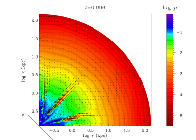
Figure 6: Example of an axisymmetric hybrid inflow-outflow solution. Displayed are the distribution of gas pressure (colour map) and the velocity field (arrows) at $4.9\times 10^{7}$ yr, which forms in response to the random velocity perturbation shown in Fig. 5. The colour bar labels give $p$ on a logarithmic scale in arbitrary units.

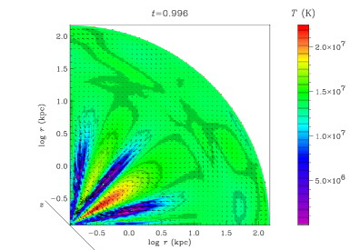
Figure 7: Same as Fig. 6, but showing the gas temperature (on a linear scale).

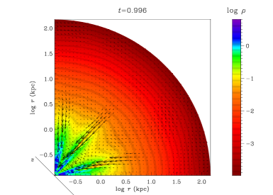
Figure 8: Same as Fig. 6, but showing the logarithm of the gas number density in units of 0.28 cm^-3.

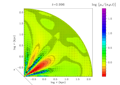
Figure 9: Same as Fig. 6, but showing the logarithm of the normalized deposited gas density.

Figure 10: Velocity field in the central region at $t=4.9\times 10^{7}$ yr.

The pressure distribution in the leftmost funnel is rather patchy. The corresponding features can also be seen in the velocity map (Fig. 10). The gas tends to concentrate in radially compressed clumps, where it condenses out digging a low pressure channel into the hot galactic atmosphere. As a result a radial hollow jet of high velocity gas forms. Growing from linear values of about 100 km s^-1 at $t=0.85\>t_{\mathrm{s,0}}$ the maximum flow velocity saturates at a slightly supersonic [in relation to $c(T_{\mathrm{eq}})$] value of $\leq 700$ km s^-1 when the temperature in the funnels drops to $\sim 10^{6}$ K.

The inflow-outflow boundary represents a tangential discontinuity. In an ideal fluid such discontinuities are absolutely unstable even with respect to infinitely small perturbations [Landau & Lifshitz 1959]. The growth rate of this shear instability, ${\mathrm{Im}}(\omega)$, depends on the wavenumber of the instability, the relative velocity $v_{\mathrm{r}}$ of the fluids and on the densities of both fluids

$${\mathrm{Im}}(\omega)=kv_{\mathrm{r}}{\sqrt{\rho_{1}\rho_{2}}\over\rho_{1}+\rho_{2}}.$$ (29)

On time-scales of $\sim 0.1\>t_{\mathrm{s,0}}$ perturbations with a wavelength

$$\lambda\leq\lambda_{\mathrm{crit}}=0.6{v_{\mathrm{r}}\over 100\>\mathrm{km\>s}^{-1}}{\sqrt{\delta\rho}\over 1+\delta\rho}\;\>{\mathrm{kpc}},$$ (30)

where $\delta\rho\equiv{\rho_{1}\over\rho_{2}}$, become non-linear. However, our case is considerably more complex, since in the non-linear regime compressibility effects are important and since the instability of the tangential discontinuity can be coupled with the condensational instability driven by the sources. Nevertheless, one can still obtain a rough estimate from equation (30). For a typical density contrast $\delta\rho=0.1$ and a relative flow speed $v_{\mathrm{r}}=400$ km s^-1 one finds $\lambda_{\mathrm{crit}}=0.7$ kpc. This implies that the instability may be important for the further evolution of the streams.

The temperature map (Fig. 7) shows that the initial isothermal gas distribution gets destroyed by the perturbations. The funnels are filled by cooler gas with temperatures as low as $10^{6}$ K, while in the outflow regions the gas is hotter than in the equilibrium ($T\approx 2\times 10^{7}$ K). Note, that although periodic boundary conditions are applied in angular direction, there exists no high temperature region between the leftmost and (the periodically continued) rightmost funnel. Instead, there are indications of a temperature drop and inflow in the inter-funnel region. This may be considered as an indication of an imminent coalescence of the two evolved funnels, because of the same reason as in the case of the coalescence of condensation fronts described in [Kritsuk 1998]. However, in the realistic three-dimensional case the probability for such a coalescence of two finger-like streams must be quite low. It seems that at least the hot, well structured outflow region between the central and the rightmost funnel will prevent them from merging.

Figure 11: Example of an axisymmetric hybrid inflow-outflow solution at $t=4.9\times 10^{7}$ yr. Displayed are various angular-averaged variables. See also Fig. 1.

The (number) density map (Fig. 8) looks qualitatively similar to the pressure map. Different stages of gas compression and deposition can be seen in the three funnels. The maximum number density is 1.7 cm^-3. Such large values are reached in the condensing fragments falling down towards the centre.

The map of the normalized mass density (Fig. 9) deposited during the simulation is similar to the temperature map. Gas condensation was much more efficient in the funnels, while in the outflow regions the rate falls below the equilibrium values. The condensation pattern in the forming streams looks rather patchy. This indicates once again that during the development of the streams the gas cools and condenses out in clumps. With an initial number density of 1.0 cm^-3 and a size of 0.2 kpc the mass of such a clump, $\sim 10^{6}$ M_⊙, corresponds to the mass of a globular cluster.

Apparently, the presence of hollow jets, which fill only a small fraction of the whole volume in the central parts of a galaxy, does not change the X-ray observables dramatically as compared to those of the equilibrium gas configuration, if individual streams cannot be resolved well. To demonstrate this we show in Fig. 11 angular averages of the same variables, which were plotted for spherically symmetric flows in Figs 1-4. The mean temperature is averaged with a weight $\rho^{2}$, while we use a $\rho$-weighted mean for the radial velocity. We find that, at least at $t=1.0\>t_{\mathrm{s,0}}$, the density and surface brightness profiles do not differ substantially from the equilibrium ones. The mean temperature drops by $\sim 50$ % towards the centre showing some oscillations due to individual cooling clumps. Weighted mean inflow velocities up to $\sim 10^{2}$ km s^-1 indicate substantial deviations from hydrostatic equilibrium. [The adiabatic sound velocity at the equilibrium temperature is $c(T_{\mathrm{eq}})\approx 555$ km s^-1.] At the same time, the bulk ($\sim 50\%$) of the condensed gas mass is deposited in the very center of the galaxy, $r\leq 2$ kpc, and the mass deposition rate within the cooling radius is comparable to that of the spherically symmetric inflows shown in Figs 1 and 3.

These results suggest that in the absence of direct gas velocity measurements the interpretation of the surface brightness and the temperature profile in terms of the quasi-hydrostatic steady-state approximation built into the ‘standard’ cooling flow model can easily result in an erroneous spatial distribution of the mass deposition rate $\dot{M}(r)$. Violation of hydrostatic equilibrium in a small fraction of the volume, filled with accelerated gas streams, can lead to a considerable mass flux of gas towards the centre, while the bulk of the hot galactic corona remains in a quasi-equilibrium state.

Because of the extremely short cooling time scale in the blobs near the centre, we cannot simulate the development of the instability into the non-linear regime for a long time. The final fate of the evolving perturbations, thus, remains unclear at this stage of the study. It is hard to predict whether the formation of funnels represents just the onset of a forthcoming global cooling catastrophe at the centre or whether the funnels are transient features, which will be destroyed by hydrodynamic instabilities. Feedback heating could play an important role in saturating the instability in the non-linear regime, but the definition of feedback is uncertain.

6 Discussion

We found solutions, which can be classified in four different types:

• A subsonic outflow with temperature enhancement in the central region ${\Delta T\over T}\sim 3$ with typical gas velocities of about 200 km s^-1 and a low X-ray luminosity;

• A quasi-hydrostatic gas configuration with outflow velocities $\sim 10$ km s^-1, a nearly isothermal gas distribution, and X-ray observables close to those of the recycling model;

• An unstable spherically symmetric inflow with a X-ray luminosity considerably exceeding observed values;

• A hybrid inflow-outflow solution with a temperature depression in the center, mean inflow velocities of $\sim 100$ km s^-1, and a X-ray brightness distribution similar to the one of the recycling model.

The prototypes are given in Figs 2, 4, 1$+$3, and 11, respectively.

Since the spherically symmetric non-linear regime of catastrophic cooling is unstable, we consider solutions of type (iii) as being not realized in nature. The other three types represent flow regimes, which can be expected to occur in galaxies, depending on the degree of suppression of thermal conductivity in the hot ISM and on the source of the large-scale perturbations.

According to a simple scenario, the hot ISM evolves through several stages with a galaxy free of any gas in the beginning: (1) a supersonic galactic wind driven by early SN activity, (2) a slow outflow regime, and (3) an inflow, triggered by the central cooling catastrophe; see [Ciotti et al. 1991]. The evolution is driven by coordinated secular changes of the control parameters which determine the mass loss rate and the characteristic temperature of the distributed heat source in the galaxy, $\alpha(t)$ and $T_{0}(t)$. Since the study of Ciotti et al. (1991) does not include the mass deposition due to local thermal instabilities in the ISM, one can speculate, that their inherently unstable (either to wind or to inflow) outflow regime, probably, corresponds to our, in the same sense unstable, equilibrium recycling model. In our case the hot ISM in elliptical galaxies could be accumulating to fill the potential well and to approach ‘thermodynamic’ equilibrium between sinks and sources, while the SN activity and stellar mass loss decrease. The evolution in the outflow phase near equilibrium could last for a long time before it enters the inflow phase and ends up with a cooling catastrophe. It is expected that this transition can also be triggered earlier by external or internal processes which disturb the ISM of the galaxy. However, a thorough study of the stability for evolutionary ISM models with time-dependent sources is needed in order to draw rigorous conclusions for this non-linear problem.

Our hybrid inflow-outflow solutions indicate that the central cooling catastrophe can develop in the form of radially oriented streams of low density peripheral gas penetrating the subsonic outflow. The vertical orientation of (nearly) isolated giant ellipticals is defined by the condition $t_{\mathrm{G}}\ll t_{\mathrm{c,0}}$. When the thermal and gravitational time scales are comparable in the central region, or when $t_{\mathrm{G}}>t_{\mathrm{c,0}}$, the condensation fronts will be orientated in a random way, since gravity does not focus the flows. This case is described in detail in [Kritsuk 1998]. The matter, deposited in narrow streams, can show up in optical and UV emission lines as filamentary nebulae residing within a radius of a few kpc from the nucleus. The morphology of such filaments depends both on the ratio of the characteristic thermal and free fall time scales and on the topological properties of the large-scale perturbations triggering the instability. A detailed study of the dynamics of the cooling catastrophe requires multidimensional high resolution simulations, which would allow one to follow the development of the hydrodynamic instabilities further into the non-equilibrium epoch. This work is in progress.

Numerical experiments allow us to identify two modes for mass deposition in hot galactic coronae. The first, hydrostatic continuous mode, corresponds to a distributed mass deposition, as it occurs in equilibrium models and in slow or subsonic outflows. The second, dynamical mode, is related to the catastrophic cooling regime. These modes can be responsible for the diffuse blue light emission due to continuously distributed star formation of low efficiency and due to massive young star clusters formed in bursts triggered by large-scale perturbations. The amount of mass deposited in both ways can be comparable. However, the mean $\dot{\rho}_{\mathrm{ti}}(r)$ distribution follows the density of the old stellar population in the quiescent mode, while it is much more concentrated towards the centre in case of the catastrophic mode.

Currently our study does not include the effects of an additional intra-cluster gas component, which typically has a considerably higher temperature corresponding to the cluster gravitational potential. The intra-cluster medium can serve as a thermal energy reservoir for the ISM of the galaxy and it can essentially modify the gas dynamics through the enhanced pressure at the outer boundary. We will address these problems in a subsequent publication. On the other hand, slow rotation and flattening of the galactic gravitational potential do introduce finite perturbations to the equilibrium model. Hence, one expects a hybrid solution with inflow along the equatorial plane and with polar outflows. Recent results of D’Ercole & Ciotti (1997) have clearly demonstrated that this is indeed the case.

7 Conclusions and perspective

Using numerical technique we probed the stability of the hydrostatic equilibrium recycling model for hot gaseous coronae of giant elliptical galaxies with respect to a variety of perturbations.

In the absence of heat conduction the equilibrium appears to be unstable on a time scale of the order of the thermal time for the gas at the galactic centre. The physical reason for this instability is rooted in the properties of the source terms. The energy and mass sinks due to local thermal instabilities essentially modify the elastic properties of the gas. A slow contraction of a gas element amplifies the condensation and cooling in it and, thereby, the mass inflow into the compressed region. As a result, the density rises, providing further growth of losses and accelerating the contraction in a runaway regime. A slow expansion of the gas element instead decreases the losses and increases the specific heating per unit mass, which further decreases the losses and accelerates the element expansion. The expansion and heating saturate as the gas temperature approaces the characteristic temperature of the heat source. Both types of unstable behaviour can be identified in our simulations.

Spherically symmetric perturbations trigger either gas inflow, which ends up with a cooling catastrophe in the core of a galaxy, or a subsonic outflow regime, which efficiently removes the gas from the central region. In the first case the X-ray surface brightness at the centre of the galaxy considerably exceeds observed values, while in the second case the hot gas is practically invisible in X-rays.

Thermal conduction is able to maintain a stable equilibrium only against low-amplitude perturbations. Spherically symmetric, global density perturbations with amplitudes $\geq 10$ % remain unstable. In case of inflows the conductive heat flux cannot prevent the cooling catastrophe at the centre, but can delay it in time considerably. On the other hand, when the thermal conductivity is not suppressed, the gas velocities of outflows saturate at much lower values. This gives rise to quasi-steady-state solutions with an X-ray luminosity only slightly lower than that of the equilibrium model.

Using axisymmetric perturbations, we were able to study the 2D hydrodynamics of the cooling catastrophe for the first time. In axial symmetry the system exhibits an qualitatively different behaviour. A set of narrow cooling gas streams, flowing towards the centre through a global subsonic galactic wind, develops in response to random velocity perturbations of the equilibrium recycling model. In the strongly non-linear regime the characteristic averaged X-ray observables of such hybrid gas flows (e.g., the surface brightness and the temperature profiles) mimic the characteristics of the initial equilibrium state, while the equilibrium itself appears to be considerably violated.

These results indicate the need for a three-dimensional time-dependent treatment of the problem, which would be able to reveal non-linear instability saturation mechanisms. At the same time, they cast doubts on using steady-state ‘cooling flow’ type models, based on the assumption of quasi-hydrostatic equilibrium, for recovering mass deposition rates in the central galactic regions.

References

- [Anders & Grevesse 1989] Anders E., Grevesse N., 1989, Geochim. Cosmochim. Acta, 53, 197.
- [Brighenti & Mathews 1997] Brighenti F., Mathews W., 1997, ApJ, 486, L83
- [Buson et al. 1993] Buson L. M. et al., 1993, A&A, 280, 409
- [Caldwell 1984] Caldwell N., 1984, PASP, 96, 287
- [Canizares et al. 1987] Canizares C. R., Fabbiano G., Trinchieri G., 1987, ApJ, 312, 503
- [Cappellaro et al. 1997] Cappellaro E., Turatto M., Tsvetkov D.Yu., Bartunov O.S., Pollas C., Evans R. Hamuy M., 1997, A&A, 322, 431
- [Ciotti et al. 1991] Ciotti L., D’Ercole A., Pellegrini S., Renzini A., 1991, ApJ, 376, 380
- [Colella & Woodward 1984] Colella P., Woodward P. R., 1984, J. Comput. Phys., 54, 174
- [David et al. 1990] David L. P., Forman W., Jones C., 1990, ApJ, 359, 29
- [David et al. 1991] David L. P., Forman W., Jones C., 1991, ApJ, 369, 121
- [Davis & White 1996] Davis D.S., White III R.E., 1996, ApJ, 470, L35
- [Demoulin-Ulrich et al. 1984] Demoulin-Ulrich M. H., Butcher H. R., Boksenberg A., 1984, ApJ, 285, 527
- [D’Ercole et al. 1989] D’Ercole A., Renzini A., Ciotti L., Pellegrini S., 1989, ApJ, 341, L9
- [D’Ercole & Ciotti 1997] D’Ercole A., Ciotti L., 1997, ApJ, in press, astro–ph/9710011
- [Donnelly et al. 1990] Donnelly R. H., Faber S. M., O’Connell R. M., 1990, ApJ, 354, 52
- [Eskridge et al. 1995] Eskridge P.B., Fabbiano G., Kim D.-W., 1995, ApJ, 442, 523
- [Faber & Gallagher 1976] Faber S. M., Gallagher J. S., 1976, ApJ, 204, 365
- [Forman et al. 1979] Forman W., Jones C., Liller W., Fabian A. C., 1979, ApJ, 234, L27
- [Forman et al. 1985] Forman W., Jones C., Tucker W., 1985, ApJ, 293, 102
- [Godunov 1959] Godunov S. K., 1959, Matematicheskii Sbornik, 47, 271
- [Godunov et al. 1961] Godunov S. K., Zabrodin A. V., Prokopov G. P., 1961, Zh. Comp. Math. and Math. Phys., 1, 1020
- [Jura et al. 1987] Jura M., Kim D. W., Knapp G. R., Guhathakurta P., 1987, ApJ, 312, L11
- [Kritsuk 1992] Kritsuk A. G., 1992, A&A, 261, 78
- [Kritsuk 1996] Kritsuk A. G., 1996, MNRAS, 280, 319
- [Kritsuk 1997a] Kritsuk A. G., 1997, MNRAS, 284, 327
- [Kritsuk 1997b] Kritsuk A. G., 1997, in da Costa L.N., Renzini A., eds, Proc. ESO-VLT Workshop, Galaxy Scaling Relations: Origins, Evolution and Applications. Springer-Verlag, Heidelberg, p. 356
- [Kritsuk 1998] Kritsuk A. G., 1998, to appear in Astron. Lett.
- [Landau & Lifshitz 1959] Landau L.D.& Lifshitz E.M., Theoretical Physics, Vol. VI, Fluid Mechanics, Pergamon Press Ltd.. Oxford, 1959
- [Macchetto et al. 1996] Macchetto F., Pastoriza M., Caon N., Sparks W. B., Giavalisco M., Bender R., Capaccioli M., 1996, A&AS, 120, 463
- [Mathews 1990] Mathews W. G., 1990, ApJ, 354, 468
- [Matsumoto et al. 1997] Matsumoto H., Koyama K., Awaki H., Tsuru T., Loewenstein M., Matsushita K., 1997, ApJ, 482, 133
- [Meiksin 1988] Meiksin A., 1988, ApJ, 334, 59
- [Murray & Balbus 1992] Murray S. D., Balbus S. A., 1992, ApJ, 395, 99
- [Phillips et al. 1986] Phillips M. M., Jenkins C. R., Dopita M. A., Sadler E. M., Binette L., 1986, AJ, 91, 1062
- [Sarazin & Ashe 1989] Sarazin C. L., Ashe G. A., 1989, ApJ, 345, 22
- [Sarazin & White 1988] Sarazin C. L., White III R. E., 1988, ApJ, 331, 102
- [Sarazin & White 1987] Sarazin C. L., White III R. E., 1987, ApJ, 320, 32
- [Singh et al. 1995] Singh K. P., Bhat P. N., Prabhu T. P., Kembhavi A. K., 1995, A&A, 302, 658
- [Spitzer 1962] Spitzer L., 1962, Physics of Fully Ionized Gases. Interscience, New York
- [Sutherland & Dopita 1993] Sutherland R. S., Dopita M. A., 1993, ApJS, 88, 253
- [Thomas et al. 1986] Thomas P. A., Fabian A. C., Arnaud K. A., Forman W., Jones C., 1986, MNRAS, 222, 655
- [Trinchieri et al. 1986] Trinchieri G., Fabbiano G., Canizares C. R., 1986, ApJ, 310, 637
- [van den Bergh & Tammann 1991] van den Bergh S., Tammann G. A., 1991, ARA&A, 29, 363
- [van Leer 1979] van Leer B., 1979, J. Comput. Phys., 32, 101
- [Vedder et al. 1988] Vedder P. W., Trester J. J., Canizares C. R., 1988, ApJ, 332, 725