A Tale of Two SZ Sources

Abstract

The recent discovery of two flux decrements in deep radio maps obtained by the VLA and the Ryle Telescope can have powerful implications for the density parameter of the Universe, $\Omega_{\rm o}$. We outline these implications by modeling the decrements as the thermal Sunyaev–Zel’dovich (SZ) effect from two clusters assuming their properties are similar to those of the low redshift population. In this case, the absence of any optical or X–ray counterparts argues that the clusters must be at large redshifts. We highlight the difficulty this poses for a critical cosmology by a comparison with a fiducial open model with $\Omega_{\rm o}=0.2$ ($\lambda_{\rm o}=0$). Applying the phenomenological X–ray luminosity–temperature relation needed to explain the EMSS cluster redshift distribution, as inferred by Oukbir and Blanchard (1997), we convert the X–ray band upper limits to lower limits on the clusters’ redshifts. Comparison of the counts implied by these two SZ detections with model predictions, for clusters with redshifts larger than these lower limits, illustrates quantitatively the inability of the critical cosmology to account for such high–redshift clusters. On the other hand, the open model with $\Omega_{\rm o}=0.2$ remains consistent with the existence of the two objects; it possibly has, however, difficulties with current limits on spectral distortions and temperature fluctuations of the cosmic microwave background. The discussion demonstrates the value of SZ cluster searches for testing cosmological models and theories of structure formation.

1 Introduction

Most favored theories of structure formation in the Universe are based on the gravitational growth of initially small density perturbations with Gaussian statistics. The Gaussian characteristic finds its way into the mass function of cosmic structures and leads to the expectation of an exponentially rapid decline in the number density of objects with increasing mass (Press & Schechter PS (1974)). The interesting consequence is that the abundance of massive objects, such as galaxy clusters, is then extremely sensitive to the power spectrum (amplitude and shape) of the density fluctuations and their growth rate with redshift. Since the growth rate is controlled by the density parameter of the Universe, $\Omega_{\rm o}$, this means that the shape of the redshift distribution of clusters of a given mass is sensitive to $\Omega_{\rm o}$. In fact, once constrained by local data, the redshift distribution depends only on the underlying cosmology, i.e., $\Omega_{\rm o}$ (and to a lesser extent, on the cosmological constant $\Lambda$). In other words, the redshift distribution provides a probe of the density of the Universe (Oukbir & Blanchard OB0 (1992), OB (1997); Blanchard & Bartlett b2 (1997)). The sense is such that we expect many more clusters at large redshift if $\Omega_{\rm o}<1$, because the growth rate is suppressed by the rapid expansion at late times in open models, leading to less evolution towards the past.

Essential for the application of this probe of $\Omega_{\rm o}$ is the existence of an easily observed cluster quantity well correlated with virial mass. It has been cautioned by many authors that the velocity dispersion of cluster member galaxies is too easily inflated by contamination of interlopers along the line–of–sight (e.g., Lucy interlop1 (1983); Frenk et al. interlop2 (1990); Bower et al. interlop3 (1997)). Many have turned instead to the X–ray temperature of the intracluster medium (ICM). On theoretical grounds, it is believed that the gas is heated by infall to the virial temperature of the cluster gravitational potential well. Numerical simulations in fact support the existence of a tight relation between virial mass and X-ray, which is to say, emission weighted, temperature (Evrard Tsim1 (1990); Evrard et al. Tsim2 (1996)). The dependence of the relation is as expected based on the idea that the gas is shock heated to the virial temperature on infall, although the simulations indicate that there is an incomplete thermalization of the gas, resulting in a temperature slightly ($\sim 20\;$ %) smaller than the virial value. The X–ray temperature is to be preferred over the X–ray luminosity as an indicator of virial mass, because the X–ray luminosity depends not only on the temperature, but also on the quantity of gas and on its density, or, what is equivalent, the spatial distribution of the ICM. This spatial distribution is difficult to model, particularly because there is at present no understanding of the origin of the ICM core radius.

Use of the X–ray temperature function to constrain models of structure formation is rather well developed as a subject (e.g., see Bartlett casa (1997) and references therein). Temperature data on clusters at $z>0$ is just now becoming available, and the possibility of even higher $z$ data from future space missions like XMM makes the application of the redshift distribution test proposed by Oukbir & Blanchard a real possibility over the near term (see, e.g., Sadat et al. SBO (1997)).

The Sunyaev–Zel’dovich (SZ) (Sunyaev & Zel’dovich SZ (1972)) effect offers another, complimentary approach to the problem of applying mass function evolution as a probe of $\Omega_{\rm o}$. Due to the distance independence of the surface brightness of the distortion, the effect represents an efficient method of finding high redshift clusters. This should be contrasted with X–ray emission, whose surface brightness suffers the $(1+z)^{-4}$ cosmological dimming. Moreover, as will be developed below, the SZ effect has other, important advantages over X–ray studies: the integrated SZ signal of a cluster, its flux density (measured in Jy), is proportional to the total hot gas mass times the particle weighted temperature. This means that the signal is independent of the gas’ spatial distribution and that the temperature involved is closely tied to the cluster virial mass, by energy conservation during collapse, for it is simply the total energy of the system divided by the number of gas particles. For the same reason, this temperature should also be much less sensitive to any temperature structure in the gas than the X–ray (emission weighted) temperature. Thus, the SZ effect is an observable which combines ease of theoretical modeling with ease of detection at large $z$.

All of this has prompted several calculations of the expected SZ number counts and redshift distribution of SZ selected clusters, and their dependence on the cosmological parameters and ICM evolution (Korolyov et al. SZcounts1 (1986); Bartlett & Silk SZcounts2 (1994); Markevitch et al. SZcounts3 (1994); Barbosa et al. SZcounts4 (1996); Eke et al. Tcon8 (1996); Colafrancesco et al. SZcounts5 (1997)). The future of this kind of study appears bright with the prospect of the Planck Surveyor satellite mission (http://astro.estec.esa.nl/Planck/). Ground based efforts have also made astounding progress recently, and it is already feasible to map $\sim 1$ square degree of sky to produce number counts down to flux levels sufficient to test theories (Holzapfel, private communication).

In this paper, we discuss what may already be an indication of clusters at very large redshift and the resulting implications. We refer to two radio decrements, one found in a deep VLA field (Richards et al. vla:radio (1996)) and the other detected by the Ryle Telescope during an observation of a double quasar system (Jones et al. ryle:radio (1996)). Although these detections await definitive confirmation, we will nevertheless proceed to outline here the implications of their explanation as the thermal SZ effect produced by two clusters. What makes just two such objects of great importance is the fact that no optical or X–ray counterparts have been observed, and the flux limits in the X–ray are so stringent that the clusters would have to be at large redshift (Richards et al. vla:radio (1996); Kneissl kneissl1 (1997); Kneissl et al. kneissl2 (1998)). This is of paramount importance because, as we have mentioned, massive clusters (say $M\geq 10^{15}$M_⊙) at large $z$ are not expected in critical models. Our goal in this paper is to quantify just how badly critical models fare in this regard. We emphasize that the modeling is based on the observed characteristics of the galaxy cluster population, in particular the X–ray luminosity–temperature relation and constraints on its potential evolution. This excludes from the present discussion the possibility of a large class of low luminosity clusters (both optical and X–ray). We believe that a clear discussion in this restricted context is nevertheless useful. (For this reason we dubb this work a “tale”!). The procedure also demonstrates the great potential of SZ cluster searches for constraining theories of structure formation.

The plot of the tale proceeds as follows: In the next section, we introduce the two radio decrements and their properties which will be used later. Then we outline our modeling of the SZ cluster population and of the two radio decrements. This is followed by a discussion of the X–ray emission to be expected from clusters producing the observed SZ signals and the minimum redshifts imposed by the X–ray flux upper limits; this represents a key element of our tale. Finally, we discuss the results and various caveats in the analysis before bringing an end to the tale with a brief summary.

2 The Two Sources

One of the cluster candidates was discovered in a deep VLA pointing of an HST Medium Deep Survey field (Richards et al. vla:radio (1996)). Near the center of the pointing, a radio flux decrement was detected with an extension of around $30\times 60\;$ sq. arcsecs. The integrated (negative) flux is about $-27\pm 6.6\;\mu{\rm Jy}$ at the observation frequency of 8.44 GHz (recall that Jy $=10^{-23}$ ergs/s/cm²/Hz). In what follows, we will scale all SZ fluxes to their value at the emission peak of the effect, $\lambda=0.75$ mm. In these terms, this object is a source of $(4.2\pm 1)$ mJy. The other possible cluster was found during a Ryle Telescope (RT) observation in the direction of the quasar pair PC1643+4631A,B (Jones et al. ryle:radio (1996)), as part of the telescope’s ongoing effort to find high-z clusters (Saunders ryle:prog (1997)). This object is slightly larger and stronger, corresponding to an integrated flux decrement of $-410\pm 64\;\mu{\rm Jy}$ at 15 GHz and extending over an area of $110\times 175\;$ sq. arcsecs. Translating to our fiducial frequency, we find a source of $(19.64\pm 3)$ mJy.

The crucial aspect of these two candidates is that, despite somewhat extensive efforts, no optical or X–ray counterpart has been identified (Richards et al. vla:radio (1996); Saunders et al. ryle:optical (1997)). We will focus on the implications of the X–ray data. The VLA field has been observed by the HRI aboard ROSAT, achieving a limiting sensitivity of $\sim 2\times 10^{-14}\;$ ergs/s/cm² in the band [0.1,2.4] keV. A similar limit on the bolometric flux (converted using $T=2.5\leavevmode\nobreak\ {\rm keV}$) has been set on the RT candidate (Kneissl kneissl1 (1997); Kneissl et al. kneissl2 (1998)), in what was one of the last PSPC pointings made with ROSAT. Thus, in both cases, no X–ray emission is detected down to very faint flux levels.

3 Modeling the SZ Effect

In this section we discuss, first, our modeling of the cluster counts and redshift distribution as a function of the total, integrated SZ flux, i.e., assuming that the clusters are unresolved. This has the advantage that the results are independent of the gas distribution, as already remarked. However, the actual observations may in fact be resolving the supposed clusters, depending upon their redshift. We must therefore model the gas distribution in order to interpret the observations. We discuss this aspect in the second subsection; we will argue that the singular isothermal sphere represents the most favorable case for a critical universe.

3.1 SZ Counts and Redshift Distribution

Our notation and approach follow that described in Barbosa et al. (SZcounts4 (1996)). The SZ surface brightness at position $\@vec{\theta}$ is expressed as

$$i_{\nu}(\@vec{\theta})=y(\@vec{\theta})j_{\nu}(x),$$ (1)

where $x\equiv h_{p}\nu/kT_{\rm o}$ is a dimensionless frequency expressed relative to the energy of the unperturbed CMB Planck spectrum at $T_{\rm o}=2.728\;$ K (Fixsen et al. cmb:temp1 (1996)). The function $j_{\nu}$ describes the spectral shape of the effect:

$$j_{\nu}(x)=2\frac{(kT_{\rm o})^{3}}{(h_{p}c)^{2}}\frac{x^{4}\mbox{e}^{x}}{(\mbox{e}^{x}-1)^{2}}\left[\frac{x}{\tanh(x/2)}-4\right]$$

$$\equiv 2\frac{(kT_{\rm o})^{3}}{(h_{p}c)^{2}}f_{\nu}.$$ (2)

Planck’s constant is written in these expressions as $h_{p}$, the speed of light in vacuum as $c$, and Boltzmann’s constant as $k$. Notice the introduction of the dimensionless spectral function $f_{\nu}$.

An integral of the pressure through the cluster (at position $\@vec{\theta}$ relative to the center) determines the magnitude of the effect; this integral is referred to as the Compton–$y$ parameter:

$$y\equiv\int\mbox{d}l\frac{kT}{m_{e}c^{2}}n_{e}\sigma_{T},$$ (3)

where $T$ is the temperature of the ICM (really, the electrons), $m_{e}$ is the electron rest mass, $n_{e}$ the ICM electron density, and $\sigma_{T}$ is the Thompson cross section.

Finally, the quantity of primary interest to us is the total, integrated flux density from a cluster:

$$S_{\nu}(x,M,z)=j_{\nu}(x)D_{a}^{-2}(z)\int\mbox{d}V\frac{kT(M,z)}{m_{e}c^{2}}n_{e}(M,z)\sigma_{T}$$

$$\propto M_{\rm gas}<T>.$$ (4)

In this expression, $D_{a}(z)$ is the angular–size distance in a Friedmann–Robertson–Walker metric –

$$D_{a}(z)=2H_{\rm o}^{-1}c\left[\frac{\Omega_{\rm o}z+(\Omega_{\rm o}-2)(\sqrt{1+\Omega_{\rm o}z}-1)}{\Omega_{\rm o}^{2}(1+z)^{2}}\right]$$

$$\;=2H_{\rm o}^{-1}cD(z),$$ (5)

where we introduce the dimensionless quantity $D(z)$. The Hubble constant is denoted by $H_{\rm o}$ and will also be referred to by its dimensionless cousin $h\equiv H_{\rm o}/100$ km/s/Mpc. Unless otherwise specified, we use $h=1/2$. Notice that the integral over the virial volume has reduced our expression to a product of the total gas mass times a temperature. This is the origin of the statement that the effect is independent of the ICM spatial distribution – it depends only on the total gas mass. The formal definition of the temperature in the expression is $<T>\propto(1/M_{\rm gas})\int dVn_{e}T$, which is the mean, particle weighted temperature, i.e., the total thermal energy of the gas divided by the total number of gas particles. Even more so than the X–ray temperature, which is emission weighted, this quantity is expected to have a tight correlation with cluster virial mass, just based on energy conservation during collapse; it is also much less sensitive to any temperature structure in the ICM. In addition, there is the well known fact that the SZ surface brightness, Eq. (1), is independent of redshift, assuming constant cluster properties; thus, clusters may be found at large redshift, whereas the X–ray surface brightness suffers from ‘cosmological dimming’. We emphasize the fact that SZ modeling has these important advantages over modeling based on cluster X–ray emission.

Table
Model Parameters - normalized to the local X–ray temperature function^a

$\Omega_{\rm o}$	$h$	$\sigma_{8}$	$n$
0.2	0.5	1.37	-1.10
1.0	0.5	0.61	-1.85

$a$ - Henry & Arnaud (HA (1991))

Assuming the X–ray temperature and the SZ temperature are the same, we may insert the T–M relation, tested by numerical simulations (Evrard Tsim1 (1990); Evrard et al. Tsim2 (1996)), into our flux density expression to obtain

$$S_{\nu}=(8\,\mbox{\rm mJy}\,h^{8/3})f_{\nu}(x)f_{\rm gas}\Omega_{o}^{1/3}M_{15}^{5/3}[\frac{\Delta(z)}{178}]^{1/3}$$

$$(1+z)D^{-2}(z),$$ (6)

which depends on the total virial mass ($M_{15}\equiv M/10^{15}\;\rm\,M_{\odot}$), the gas mass fraction, $f_{\rm gas}$, and the redshift of the cluster. Other quantities appearing in this equation are the mean density contrast for virialization, $\Delta(z,\Omega_{\rm o},\lambda_{\rm o})$ ($=178$ for $\Omega_{\rm o}=1$, $\lambda_{\rm o}=0$), and the dimensionless functions $f_{\nu}$ and $D(z)$ introduced in Eqs. (3.1) and (3.1). For the time being, we will suppose that $f_{\rm gas}=0.06\;h^{-1.5}$ (Evrard gasfrac (1997)) and that it is constant over mass and redshift; we will re–address this issue later. This simplifies the discussion and will help to clearly distinguish the various important physical effects.

We may now transform the mass function, for which we shall adopt the Press–Schechter (1974) formula –

$$n(M,z)dM=\sqrt{\frac{2}{\pi}}\frac{<\rho>}{M}\nu(M,z)\left|\frac{\mbox{d}\ln\sigma(M)}{\mbox{d}\ln M}\right|\mbox{e}^{-\nu^{2}/2}\frac{dM}{M}$$ (7)

– into a number density of clusters at each redshift with a given SZ flux density. In this way, we can calculate the integrated SZ source counts and the redshift distribution of sources at a given SZ flux density. In Eq. (7), $n(M,z)$ gives, at redshift $z$, the comoving number density of collapsed objects with mass $M$, per interval of $M$. The quantity $<\rho>$ represents the comoving cosmic mass density and $\nu(M,z)\equiv\delta_{c}(z)/\sigma(M,z)$, with $\delta_{c}$ equal to the critical linear over–density required for collapse and $\sigma(M,z)$ the amplitude of the density perturbations on a mass scale $M$ at redshift $z$. More explicitly, $\delta_{c}(z,\Omega_{\rm o},\lambda_{\rm o})$ and $\sigma(M,z)=\sigma_{\rm o}(M)\times(D_{\rm g}(z)/D_{\rm g}(0))$, $D_{\rm g}(z,\Omega_{\rm o},\lambda_{\rm o})$ being the linear growth factor. It is essentially through $D_{\rm g}$ that the dependence on cosmology ($\Omega_{\rm o}$, $\lambda_{\rm o}$) enters the mass function (see, e.g., Bartlett casa (1997) for a detailed discussion).

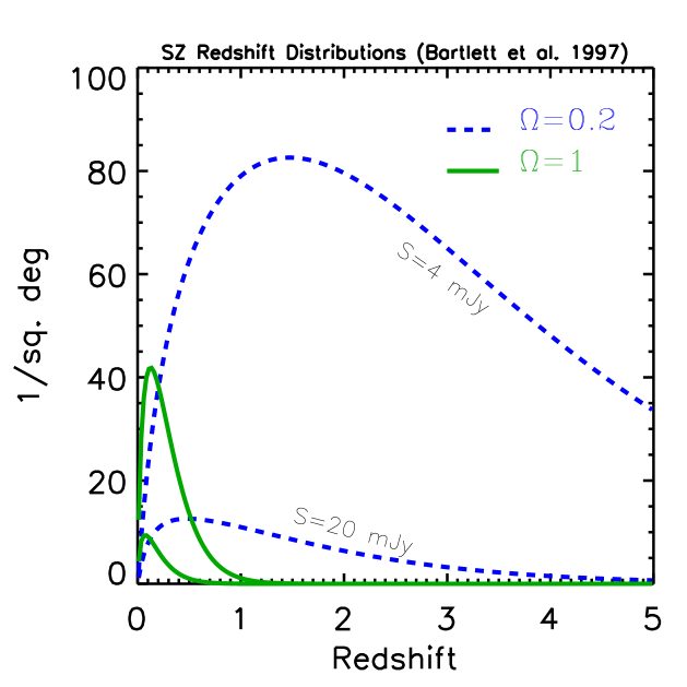
Figure 1: Redshift distribution of clusters with flux densities of 4 and 20 mJy at $\lambda=0.75$ mm. The dashed curves are for the open model. Although for clarity not explicitly labeled, the solid curves show the results for the critical model for the same flux densities. The model parameters are given in the Table, and we use $h=1/2$.

For illustration we will concentrate on the comparison of a critical model ($h=1/2$) with an open model characterized by $\Omega_{\rm o}=0.2$ ($\lambda_{\rm o}=0$ and $h=1/2$). Both are normalized to the present–day cluster X–ray temperature function. The normalization is performed by constraining, for each $\Omega_{\rm o}$, the amplitude, $\sigma_{8}$, and spectral index, $\alpha$, of an assumed power–law density perturbation power spectrum: $\sigma_{\rm o}(M)=\sigma_{8}(M/M_{8})^{-\alpha}$, where $M_{8}$ is the mass enclosed in a sphere of radius $8h^{-1}$ Mpc. In more standard terms, $\alpha=(n+3)/6$, where $n$ is the spectral index of the power spectrum: $P(k)\propto k^{n}$. The result of this normalization for the two models is given in the Table (Oukbir et al. OBB (1997); Oukbir & Blanchard OB (1997)).

The integrated cluster counts are shown in Figure 4 and discussed in Section 5, where we compare the results to the counts implied by the VLA and RT detections. Here, in Figure 1, we give the redshift distribution of clusters of fixed flux density for the two cosmologies. For flux densities comparable to those observed, we see a very large difference in the predicted number of clusters at large redshifts. Thus, the existence of even a small number of clusters at these flux levels with redshifts beyond unity can lead to extremely strong constraints on $\Omega_{\rm o}$.

3.2 Observed SZ Signals

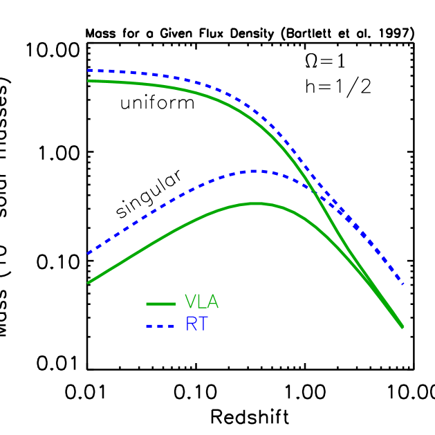
Figure 2: The virial mass required to explain each observed SZ source as a function of redshift; solid curves for the VLA, dashed for the RT. Gaussians beams of $\theta_{\rm fwhm}=1\;$ and 2 arcmins have been used for the VLA and RT, respectively. For each source, we show the results for $x_{v}=0\;$ and 500. The latter approaches a singular isothermal sphere model. In all cases $h=1/2$ and $\Omega_{\rm o}=1$.

Now let us consider the problems associated with the fact that the radio observations may be resolving the cluster candidates. We need to relate the observed, resolved SZ flux, $S_{\nu}^{\rm obs}$, to the total flux integrated over the entire cluster volume, $S_{\nu}$, which was the quantity considered in the previous subsection. To do this, we adopt the isothermal $\beta$–model for the ICM density: $n(r)\propto[1+(r/r_{c})^{2}]^{-3\beta/2}$. The only free parameter will be the core radius, $r_{c}$, because we will fix $\beta=2/3$. For the telescope beam profiles, we use Gaussians written in terms of the beam full width half maximum, $\theta_{\rm fwhm}$: $f_{\rm beam}(\theta)=\mbox{e}^{-4{\rm ln}(2)\theta^{2}/\theta_{\rm fwhm}^{2}}$, where $\theta$ is the angle relative to the beam center.

It is now possible to write down the observed fraction of the total SZ flux:

$$\xi\equiv\frac{S_{\nu}^{\rm obs}}{S_{\nu}}=\frac{\int_{0}^{x_{v}}\mbox{d}xx(1+x^{2})^{(1-3\beta)/2}\mbox{e}^{-4\ln(2)x^{2}(\theta_{c}(M,z)/\theta_{\rm fwhm})^{2}}}{\int_{0}^{x_{v}}\mbox{d}xx(1+x^{2})^{(1-3\beta)/2}}.$$ (8)

We have introduced $x_{v}\equiv R_{v}/r_{c}$, where $R_{v}(M,z)$ is the virial radius of a cluster of mass $M$ at redshift $z$. Looking at $S_{\nu}$ in Eq. (3.1) and this expression for $\xi$, it is clear that $S_{\nu}^{\rm obs}$ is a function of $M$ and $z$. Thus, as soon as the cosmological model and the characteristics of the instrument are specified, we can find, for each redshift and for given values of $x_{v}$ and $f_{\rm gas}$, the cluster mass required to produce the observed SZ flux. The results for both observations, calculated using $\Omega_{\rm o}=1$, are shown in Figure 2 for two extreme values of $x_{v}$. The telescope beams are described by $\theta_{\rm fwhm}=1$ arcmin and $\theta_{\rm fwhm}=2$ arcmins for the VLA and RT, respectively; in each case, the observed SZ source is taken to cover only one beam element. As $x_{v}\rightarrow\infty$, i.e., as $r_{c}\rightarrow 0$, we recover the singular isothermal sphere profile, while $x_{v}\rightarrow 0$ describes an uniform density isothermal sphere, truncated at $R_{v}$. Notice that because the singular profile concentrates more gas mass in the core, lower total masses are required to explain a given observation ($S_{\nu}^{\rm obs}$) than in the case of a uniform sphere. The results for $\Omega_{\rm o}=0.2$ are similar, but the corresponding curves are roughly 2–3 times larger in mass. What goes into this calculation is simply the idea that the observed radio decrements are to be explained by hot gas heated to the virial temperature of collapsed objects. Figure 2 indicates that, independent of the SZ profile, the supposed objects must have masses corresponding to groups or clusters of galaxies, as was probably expected.

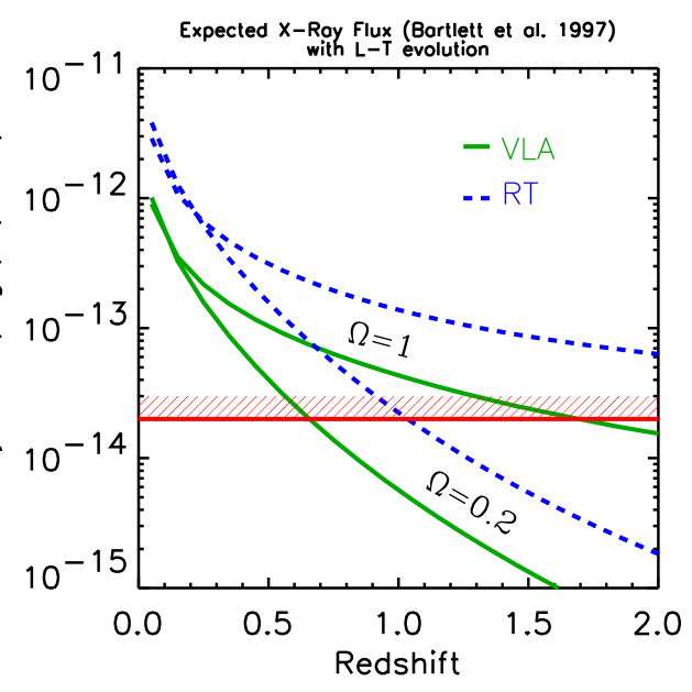
Figure 3: Expected X–ray flux for each SZ source using the evolution of $L(T)$ required to fit the EMSS redshift distribution (see text). The X–ray limits on the two fields are numerically the same, at $2\times 10^{-14}\;{\rm ergs/s/cm^{2}}$ (shown as the horizontal bar), but apply to the ROSAT [0.1–2.4] keV band for the VLA source (Richards et al. vla:radio (1996)) and to the bolometric flux for the RT source (assuming $T\sim 2.5\;$ keV – Kneissl et al. kneissl2 (1998)). The solid curves for the VLA give the in–band flux, while the dashed curves for the RT correspond to expected bolometric flux. As labeled, the upper pair of curves are for the critical model and the lower pair are for the open model.

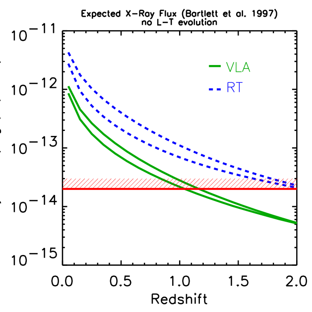
Figure 4: Same as Figure 3, but now assuming no evolution of $L(T,z)$; the observed $z=0$ relation is applied at all redshifts. In each case, the upper curve corresponds to the open cosmology, but there is very little difference between the two models.

4 Modeling the Expected X–ray Emission - turning point of the plot

The limits on X–ray emission in the two SZ fields are very stringent (and numerically similar): The ROSAT HRI places a limit of $f_{x}(0.1-2.4\;{\rm keV})<2\times 10^{-14}\;{\rm ergs/s/cm^{2}}$ on the VLA field (Richards et al. vla:radio (1996)), and a new PSPC pointing puts a limit on the bolometric flux on the RT field of $f_{x}<2\times 10^{-14}\;{\rm ergs/s/cm^{2}}$ (assuming a $T\sim 2.5\;{\rm keV}$ – Kneissl et al. kneissl2 (1998)). These tight limits suggest that the (supposed) clusters are at large redshift. Actually determining the minimum redshift thus imposed on each cluster requires some additional modeling. Fortunately, there is a phenomenological approach: as we have just seen, the SZ flux tells us the cluster temperature (or mass) for any assumed redshift. We wish to associate an X–ray luminosity to this temperature or, in other words, we are looking for a relation $L(T,z)$. Within a given cosmological model (i.e., given $\Omega_{\rm o}$), this relation is tantamount to specifying the redshift distribution of a flux limited cluster catalog, because it tells us the luminosity of clusters of a given mass, whose abundance at any redshift is given by the mass function. Oukbir & Blanchard (OB (1997)) have modeled the redshift distribution of the EMSS (Einstein Medium Sensitivity Survey, Gioia et al. EMSS (1990)) cluster sample and have shown that in fact the $L(T,z)$ relation can be used as a probe of $\Omega_{\rm o}$ in this way, because once known, $L(T,z)$ permits one to infer the evolution of the mass function (see introduction). Although determined at $z=0$, the evolution of $L(T,z)$ with $z$ is not yet fully constrained; the potential to probe $\Omega_{\rm o}$ using $L(T,z)$ is the motivation for current efforts to constraint the relation at $z>0$ (Sadat et al. 1997). For our purposes here, we will use the $L(T,z)$ required to match the observed redshift distribution of the EMSS for arbitrary $\Omega_{\rm o}$:

$$L_{x}\propto(1+z)^{\beta}T^{3}$$ (9)

with

$$\beta\approx 4.\times\Omega_{\rm o}-3.$$ (10)

(Oukbir & Blanchard OB (1997); Sadat et al SBO (1997)).

We show the resulting X–ray flux for each SZ source in Figure 3. For comparison, Figure 4 presents the results if we assume no evolution in the luminosity–temperature relation; in this latter case, the X–ray flux is roughly the same for both cosmological models. Figure 3 shows that adding the evolution required to fit the EMSS distribution – Eqs. (9) and (10) – leads to a larger expected flux for the critical model. This is because clusters of a given temperature in the critical model must be brighter in the past to explain the observed number of clusters in the EMSS. The opposite is true for the open model. In any case, and regardless of whether or not we incorporate evolution in the $L-T$ relation, the X–ray limits imply that the cluster candidates must be at redshifts beyond unity for the critical model; this is the limit we will impose in the following. We also remark that this is consistent with the lack of any optical cluster candidates in the two fields, although a quantitative limit from the optical observations requires more detailed consideration. Looking at Figure 1, we expect the critical model to have difficulty accounting for the existence of clusters beyond a redshift of 1. Massive clusters at high redshift are, on the contrary, expected to be relatively common in open models, and so the two decrements should pose relatively little difficulty for our fiducial open model. We now quantify these comments.

5 The Plot Comes Together

We need to estimate the abundance of SZ sources of the kind observed. We will then be able to compare this abundance with the predictions of the two models, and the important element in this comparison will be the lower bound on the redshift imposed by the X–ray (and optical) observations. To start, we will assume that each telescope simply observed blank regions of sky in a random fashion, making the statistics easier to handle. One may argue that this applies to the VLA observations, but not for the RT detection, which deliberately pointed in the direction of a known quasar pair. Nevertheless, this will permit us to quickly see the implications, and we can refine our arguments later.

The VLA observations included two fields and found one SZ source. Using a primary beam $\theta_{\rm fwhm}=312\;$ arcsecs, we find $\Omega^{\rm VLA}_{\rm obs}=0.018\;$ deg² for the total observed solid angle. Assuming a similar sensitivity in both fields, this yields an observed surface density of $\sim 50\;$ deg^-2 for SZ sources with a flux density greater than 4.2 mJy at our fiducial wavelength of $\lambda=0.75$ mm. Poisson statistics then tell us that the 95%, one–sided confidence limits on the surface density of these objects span the range $3-263\;$ deg^-2. Following the same line of reasoning for the RT, we note that 3 fields where observed and one object was found; a primary $\theta_{\rm fwhm}=6\;$ arcmins leads to $\Omega^{\rm Ryle}_{tot}=0.034\;$ deg² and a surface density range of $2-140\;$ deg^-2 (enclosed by the one–sided, 95% confidence limits) for sources with $\sim 20\;$ mJy at $\lambda=0.75\;$ mm.

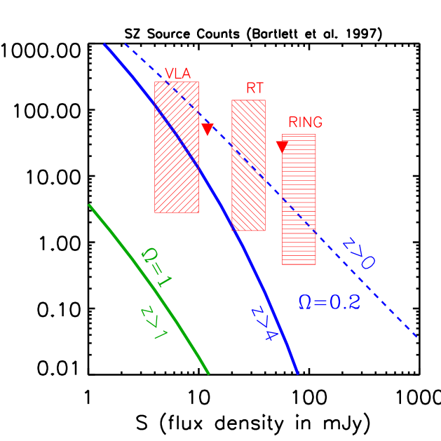
Figure 5: SZ source counts with observational constraints, as a function of SZ flux density expressed at $\lambda=0.75\;{\rm mm}$. The two hatched boxes on the left show the 95% one–sided confidence limits from the VLA and the RT; due to the uncertain redshift of the clusters, there is a range of possible total SZ flux density, which has for a minimum the value observed in each beam and a maximum chosen here to correspond to $z=1$. From the SuZIE blank fields, one can deduce the 95% upper limit shown as the triangle pointing downwards between the VLA and RT boxes (Church et al. suzie (1997)). The horizontally hatched box gives the constraints from the OVRO RING experiment (Myers et al. RING (1993)), assuming that there was one cluster detected; the triangle at the far left of this box shows the upper limit that results if, instead, one supposes that no clusters are present (see text). We overlay the predictions of our fiducial open model ($\Omega=0.2$) for all clusters (dashed line) and for those clusters with $z>4$. The critical model has great difficulty explaining the observed objects even with a lower redshift cutoff of only $z>1$; the actual limit from the X–ray data could be stronger, but this would fall well off to the lower left of the plot. We assume $h=1/2$.

In Figure 5 we compare these estimates with the predictions of the two models. The critical model shown includes clusters beyond $z=1$. Even though this is rather generous for the critical model (looking at Figures 3 and 4), it fails by a large factor to explain the counts indicated by the two radio decrements. The open model counts are shown integrated upwards from $z=0$ and from $z=4$. The open model can accommodate all the observational constraints (some of which are discussed below): clusters at $z\geq 1$ could easily produce these objects while escaping the X-ray limits. The critical model is incapable of explaining the observations, but the open model has little difficulty doing so.

6 Discussion

The principal result of this work is given in Figure 5, where we see clearly and quantitatively the difficulty faced by a critical cosmology if the VLA and RT radio decrements are representative of the cluster population’s SZ effect. We also show two other observational constraints in this figure. The SuZIE instrument recently reported no detections down to 12 mJy (at $\lambda=0.75$ mm) on blank sky covering $\Omega^{\rm SuZIE}_{tot}=0.06\;$ deg². The resulting upper limit is shown in the figure as the downward–pointing triangle between the VLA and RT boxes. The rightmost box presents one possible interpretation of the results of the OVRO RING experiment (Myers et al. RING (1993)). In this experiment, there is one field representing a $>5\;\sigma$ fluctuation and for which no source has yet been identified. If we suppose that this fluctuation is due to the SZ effect, then we deduce the constraints given by the box based on this detection, at $\sim 60$ mJy ($\lambda=0.75$ mm), over a total survey area of $\Omega_{\rm obs}^{\rm RING}=0.1\;{\rm deg^{2}}$. Once again, we give the 95% one–sided confidence limits, and the range in flux density is from the detected flux density to the corrected, total flux density for $z=1$. Alternatively, we could use the RING data as an upper limit to the source counts, arguing that this one fluctuation is not the result of a cluster. We then obtain the upper limit given as the downwards pointing arrow at the far left-hand side of the RING box.

In contrast to the critical model, our fiducial open model has no difficulty in accounting for all of the constraints shown in the figure. It is the strong upper limits on any X–ray flux from the objects, forcing them to be at large redshift (Figure 3), that makes the distinction between the two models not just a question of a factor of a few, but of orders of magnitude. The exponential behavior of the mass function provides us with large “leverage” to discriminate models at high $z$. To facilitate the presentation in the figure, we have used a lower limit of $z>1$ on the critical model, but it should be emphasized that the actual limit from Figures 3 and 4 is at least $z>2$ (for the RT), and this would put the curve completely off to the bottom left of the plot. Thus, a straightforward interpretation of the results is that the critical model is ruled out.

Let us now discuss the various caveats to this ‘straightforward’ interpretation. The first thing that must again be emphasized is that the line of argument relies heavily on the idea that the radio decrements (are real) are due to gas heated to the virial temperature of collapsed objects and that these objects behave in a manner similar to what is known about X–ray clusters. It is perhaps possible that the decrements are not due to such objects. In this case, a different approach than the one presented here is needed. The calculation in this paper was made in order to understand what the radio decrements imply if one wishes to explain them by what we know as galaxy clusters.

Even within this context, there are several issues we should address. The first is the scatter in the $L(T,z)$ relation. Arnaud and Evrard (1998) have shown that this scatter is intrinsically smaller than previously thought, by considering a cluster sample with high quality X–ray observations. The scatter is seen to be $\leavevmode\nobreak\ 20\%$ around a relation $\propto T^{2.88}$ for non–cooling flow clusters. There are, however, a couple of clusters below the mean relation and well outside the scatter. It is possible that the SZ detections are the first indication of a larger than expected population of intrinsically underluminous clusters.

Next, as already remarked, we chose for simplicity to hold the ICM gas mass fraction, $f_{\rm gas}$, constant over mass and redshift; one could imagine that it is in fact a function of both. Colafrancesco et al. (SZcounts5 (1997)) have investigated the SZ source counts including the possible effects of cluster evolution. Accounting for cluster evolution in the present context, however, will not substantially change the conclusion in respect to the critical model – we are already using, in this model, a large gas mass fraction, as supported by X–ray observations (Evrard gasfrac (1997)) (This fraction is in violation of primordial nucleosynthesis predictions for $\Omega_{\rm o}=1$, another problem for the critical model [White et al. baryoncris (1993)]). Any reasonable evolution would thus cause this fraction to decrease with either mass or redshift, or both, thereby decreasing the counts predicted by the critical model – things would get worse. One thing which could help the critical model is if the intergalactic medium surrounding the virialized region of a cluster was heated to close to 1 keV. One possible mechanism could be the diffusion of electrons through the shock front that heats the gas to the virial temperature (Chièze et al. 1997). This would increase the SZ flux density associated with a given cluster mass, pushing the predicted curves to the right. Such a mechanism could be in operation around clusters, but the factor needed to reconcile the critical model with the indicated counts seems unreasonable.

A particular source of concern is the fact that the RT object was found by observing known quasar systems, and not a priori blank fields. This seems to be less of a worry for the VLA fields, because no double quasar systems were known prior to the observations (although one was subsequently found…). We can get a feeling, at least, for the effect of a possible bias on our results in the following manner: Supposing that instead of representing random fields on the sky for a cluster search, double quasar systems are always associated with clusters (which are responsible, say, for the two images). Then another way to proceed with the RT detection would be to take the observed sky density of such double quasar systems as the SZ source counts. Over a survey area of $\sim 60\;{\rm deg}^{2}$, Schneider et al (quasdens (1994)) found 90 quasars, 3 of which are close double systems (with separations less than $\sim 400\;$ arcsecs). One of these three is in fact PC1643+4631, i.e., the RT field with the radio decrement. The implied counts are then $\sim 0.05\;{\rm deg}^{-2}$, with one–sided 95% confidence upper and lower limits of $\sim 0.13\;{\rm deg}^{-2}$ and $\sim 0.013\;{\rm deg}^{-2}$, respectively. Looking at Figure 5, we see that this will not drastically alter the severity of the critical model’s difficulty (remember that $z>2$ really applies to the RT object).

7 Summary

In summary, we have seen the possible implications of the recently discovered radio decrements in the VLA and the Ryle Telescope. If the spectra of these two objects confirm an origin in the thermal SZ effect from two galaxy clusters, then a critical model would be in serious trouble. A large part of the importance of these two objects arises from the stringent X–ray and optical limits on the two fields. This argues that the supposed clusters are at very large redshift. This has been the key, because the SZ counts (the cluster abundance) at large redshift are enormously different between a critical and an open model. While such clusters are essentially non–existent at $z>1$ in a critical model, they are to be expected in open models, even at redshifts as large as 4.

However, all is not necessarily well with the open model in light of constraints on spectral distortions and temperature fluctuations of the cosmic microwave background. Barbosa et al. (moriond (1996)) show that an open model with the power spectrum chosen here violates the FIRAS limit on $y$ (assuming a constant $f_{\rm gas}$). We may also estimate the rms temperature fluctuations created by the unresolved cluster population by applying a P-D analysis (Condon con (1974)) to our cluster counts. We find that our fiducial open model here actually violates the present limit set by the SuZIE instrument (Church et al. suzie (1997)). The significance of these shortcomings should be addressed with more careful modeling of the counts and predicted fluctuations, and with a statistical comparison more appropriate to the non-Gaussian nature of the induced temperature fluctuations (Bartlett et al., in preparation).

Our modeling of the cluster population is consistent and phenomenological in that it uses the X–ray luminosity–temperature relation required to explain the observed redshift distribution of EMSS clusters (Oukbir & Blanchard OB (1997); Sadat et al. SBO (1997)) to find the expected X–ray flux and deduce the corresponding redshift limits. The discussion has focused on the comparison between a critical model and a fiducial open model. Such a simple comparison just to highlight the possible implications seems justified at this juncture due to the preliminary nature of the data, and the procedure demonstrates the value of cluster SZ searches. We await future results with anticipation, noting for now that it is already possible to perform an SZ survey of $\sim 1\;$ square degree (Holzapfel, private communication; Holzapfel et al. suzieinst (1997)).

We would like to thank G. Djorgovski for a discussion concerning the abundance of close quasar pairs. D.B is supported by the Praxis XXI CIENCIA- BD/2790/93 grant attributed by JNICT, Portugal.

References

- (1) Arnaud M. & Evrard A.E. 1998, in preparation
- (2) Barbosa D., Bartlett J.G., Blanchard A. & Oukbir J. 1996, A&A 314, 13
- (3) Barbosa D., Bartlett J.G., Blanchard A. & Oukbir J. 1996, in: Microwave Background Anisotropies, Moriond proceedings, in press; astro-ph/9607036
- (4) Bartlett J.G. 1997, in: From Quantum Fluctuations to Cosmological Structures, School held in Casablanca, ed. D.Valls-Gabaud, M.A.Hendry, P.Molaro, K.Chamcham, A.S.P. Conf. Ser., vol. 126, p 365.
- (5) Bartlett J.G. & Silk J. 1994, ApJ 423, 12
- (6) Blanchard A. & Bartlett J.G. 1997, astro-ph/9712078
- (7) Bower R.G., Castander F. J., Couch W.J., Warrick J., Ellis, R. S. & Bohringer H. 1997, MNRAS, 291, 353
- (8) Church S.E., Ganga K.M., Ade P.A.R., Holzapfel W.L., Mauskopf P.D., Wilbanks T.M. & Lange A.E. 1997, ApJ, 484, 523
- (9) Colafrancesco S., Mazzotta P., Rephaeli Y. & Vittorio N. 1997, ApJ 433, 454
- (10) Condon J.J. 1974, ApJ 188, 279
- (11) Eke V.R., Cole S. & Frenk C.S. 1996, MNRAS 282, 263
- (12) Evrard A.E. 1990, in: Clusters of Galaxies, eds. M. Fitchett & W. Oegerle, Cambridge University Press, Cambridge
- (13) Evrard A.E. 1997, astro-ph/9701148
- (14) Evrard A.E., Metzler C.A. & Navarro J.F. 1996, ApJ 469, 494
- (15) Fixsen D.J., Cheng E.S., Gales J.M. Mather J.C., Shafer R.A., Wright E.L. 1996, ApJ 473, 576
- (16) Frenk C.S., White S.D.M., Efstathiou G. & Davis M. 1990, ApJ 351, 10
- (17) Gioia I.M., Maccacaro T., Schild R.E., Wolter A., Stocke J.T., Morris S.L. & Henry J.P. 1990, ApJS, 72, 567
- (18) Henry J.P. & Arnaud K.A. 1991, ApJ 372, 410
- (19) Holzapfel W.L., Wilbanks T.M., Ade P.A.R., Church S.E., Fischer M.L., Mauskopf P.D., Osgood D.E. & Lange A.E. 1997, ApJ 479, 17
- (20) Jones M.E., Saunders R., Baker J.C., Cotter G., Edge A., Grainge K., Haynes T., Lasenby A., Pooley G., Rẗtgering H. 1997, ApJ 479, L1
- (21) Kneissl R. 1997, in: Particle Physics and the Early Universe Conference, http://www.mrao.cam.ac.uk/ppeuc/proceedings/
- (22) Kneissl R., Sunyaev R.A. & White S.D.M. 1998, submitted to MNRAS, astro-ph/9801045
- (23) Korolyov V.A., Sunyaev R.A. & Yakubtsev L.A. 1986, Sov. Astron. Lett. 12, L141
- (24) Lucey J.R. 1983, MNRAS 204, 33
- (25) Markevitch M., Blumenthal G.R., Forman W., Jones C. & Sunyaev R.A. 1994, ApJ 426, 1
- (26) Myers S.T., Readhead A.C.S. & Lawrence C.R. 1993, ApJ 405, 8
- (27) Oukbir J. & Blanchard A. 1992, A&A 262, L21
- (28) Oukbir J. & Blanchard A. 1997, A&A 317, 1
- (29) Oukbir J., Bartlett J.G. & Blanchard A. 1997, A&A 320, 365
- (30) Press W.H. & Schechter P. 1974, ApJ 187, 425
- (31) Richards E.A., Fomalont E.B., Kellermann K.I., Partridge R.B., Windhorst R.A. 1996, astro-ph/9612183
- (32) Sadat, R., Blanchard, A. & Oukbir, J. 1997, A&A in press.
- (33) Saunders R. 1997, in: Microwave Background Anisotropies, to appear in the proceedings of the XXXIst Rencontres de Moriond, astro-ph/9611213
- (34) Saunders R., Baker J.C., Bremer M.N., Bunker A.J., Cotter G., Eales S., Grainge K., Haynes T., Jones M.E., Lacy M., Pooley G. & Rawlings S. 1997, ApJ 479, L5
- (35) Schneider D.P., Schmidt M. & Gunn J.E. 1994, AJ 107, 1245
- (36) Sunyaev R.A. & Zel’dovich Ya.B. 1972, Comm. Astrophys. Space Phys. 4, 173
- (37) Chièze, J.-P., Teyssier, R, & Alimi, J.-M., 1997, ApJ, in press, astro-ph/9709183
- (38) White S.D.M., Navarro J.F., Evrard A.E. & Frenk C.S. 1993, Nature 366, 429