A Study of the Temperature gradient in Virgo/M87 with the MECS on board Beppo-SAX

Abstract

Ground and in flight calibrations of the MECS experiment on board Beppo-SAX have demonstrated that this is currently the best X-ray imaging experiment above 3 keV. The MECS on-axis PSF has a half power radius of about 1 arcmin. Moreover due to a fortunate combination of detector and mirror PSFs the total PSF depends only weakly on the energy. Finally the degradation of the PSF with off axis angle is negligible within an off-axis angle of 10 arcminutes. Encouraged by these results we developed techniques to analyze galaxy clusters observed with Beppo-SAX. In this proceeding we quantify spectral distortions introduced by the energy dependent PSF when performing spatially resolved spectroscopy of the core of the Virgo cluster.

1 The MECS Point Spread Function

The Medium Energy Concentrator Spectrometer (MECS; Boella et al. 1997/a) is one of the four narrow field instruments on board the Beppo-SAX satellite (Boella et al. 1997/b). The MECS operates in the energy band 1.3-10 keV with a field of view of $28^{\prime}$ radius. The MECS consists of three units each composed of a grazing incidence Mirror Unit (MU), and of a position sensitive Gas Scintillation Proportional Counter (GSPC).
The Point Spread Function of the MECS (PSF_MECS) is the convolution between the MU PSF and the detector PSF. The MU and detector PSFs are described, respectively, by a lorentzian function L(r) and a gaussian function G(r). Both the lorentzian and the gaussian functions are energy-dependent. Typically the detector PSF improves with increasing energy, whereas the MU PSF improves with decreasing energy. The detector PSF dominates the core of the PSF_MECS ($r\lower 2.15277pt\hbox{$\;\buildrel<\over{\sim}\;$}2^{\prime}$) whereas the MU PSF dominates the wings of the PSF_MECS ($\lower 2.15277pt\hbox{$\;\buildrel>\over{\sim}\;$}2^{\prime}$).
The analytical expression for the on-axis PSF as given in Boella et al. 1997/a is:

$${\rm PSF_{MECS}}(r,E)=\frac{1}{2\pi\Big{[}R(E)\sigma^{2}(E)+\frac{r^{2}_{l}(E)}{2(m(E)-1)}\Big{]}}\cdot$$

$$\Bigg{\{}R(E)\exp\Bigg{(}-\frac{r^{2}}{2\sigma^{2}(E)}\Bigg{)}+\Bigg{[}1+\Bigg{(}\frac{r}{r_{l}(E)}\Bigg{)}^{2}\Bigg{]}^{-m(E)}\Bigg{\}},$$ (1)

where $R(E)$, $\sigma(E)$, $r_{l}(E)$ and $m(E)$ are algebraic functions of the energy E.
The integral of the PSF over the entire plane is normalized to unity:
$2\pi\int_{0}^{\infty}{\rm PSF_{\rm MECS}}(r,E)r\,dr\equiv 1$.
We used eq. 1 to evaluate the $50\%$ and $80\%$ power radii ($r_{50}(E)$ and $r_{80}(E)$) as a function of E:

$$2\pi\int_{0}^{r_{50}(E)}{\rm PSF_{\rm MECS}}(r,E)r\,dr=0.5,$$

$$2\pi\int_{0}^{r_{80}(E)}{\rm PSF_{\rm MECS}}(r,E)r\,dr=0.8\,.$$ (2)

Figure 1: PSF_MECS Power Radii vs. Energy. The solid line represents the 50 % power radius, r₅₀(E), the dashed line represents the 80 % power radius, r₈₀(E) (see eq. 2).

As shown in fig. 1 $r_{50}(E)$ is always $<2^{\prime}$ and decreases with increasing energy. This is because at radii $<2^{\prime}$ the PSF_MECS is dominated by the gaussian PSF of the detector, that improves with increasing energy. The power radius $r_{80}(E)$ does not vary strongly with energy (see fig. 1) because of the combined effect of the improvement of the detector PSF and degradation of the MU PSF with increasing energy.

Figure 2: Ratios between convolved profiles vs. radius r. Solid line: Ratio R₁(r) between the convolved profile $\tilde{I}$(r,3 keV) and the convolved profile $\tilde{I}$(r,6 keV). Dashed line: Ratio R₂(r) between the convolved profile $\tilde{I}$(r,9 keV) and the convolved profile $\tilde{I}$(r,6 keV)

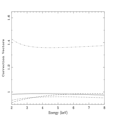
Figure 3: Correction vectors for the Virgo cluster observed with the MECS. Dot-dot-dot-dashed line: correction vector V₁(E_i) for the region $0^{\prime}-2^{\prime}$. Dashed line: correction vector $V_{2}$(E_i) for the region $2^{\prime}-4^{\prime}$. Dash-dotted line: correction vector $V_{3}$(E_i) for the region $4^{\prime}-6^{\prime}$. Dotted line: correction vector $V_{4}$(E_i) for the region $6^{\prime}-8^{\prime}$. Solid line: correction vector $V_{5}$(E_i) for the region $8^{\prime}-10^{\prime}$.

2 Convolution of the Source Radial Profile with the PSF_MECS

A proper analysis of extended sources, like clusters of galaxies, requires that the blurring introduced by the limited spatial resolution of the observing instruments be correctly taken into account. In practice, this is done by evaluating the convolution of the source surface brightness profile, $I$, with the PSF_MECS. We have approximated $I$ with the profile of the Virgo cluster as observed with the PSPC instrument on board the ROSAT satellite, because of the considerably better spatial resolution of this instrument respect to the MECS.
The ROSAT Virgo cluster profile, $I_{\rm ROSAT}(r_{0})$, convolved with the PSF_MECS at any point P($r$) in polar coordinates ($r_{0},\varphi$) is:

Figure 4: Virgo temperature profiles. The solid line is the temperature profile $T_{obs}(r)$ obtained from the observed spectrum, $S_{obs}$, whereas the dash-dotted line is the temperature profile $T_{corr}(r)$ obtained from the corrected spectrum, $S_{corr}$.

$\tilde{I}(r,E)=\int_{0}^{\infty}dr_{0}\cdot$

$$\int_{0}^{2\pi}d\varphi\,I_{\rm ROSAT}(r_{0})\,{\rm PSF_{\rm MECS}}(r,r_{0},\varphi,E)\,r_{0}\,.$$ (3)

We computed the convolved profiles $\tilde{I}(r,3{\rm keV})$, $\tilde{I}(r,6{\rm keV})$ and $\tilde{I}(r,9{\rm keV})$.
In order to estimate the spectral distortions introduced by the energy-dependent PSF_MECS we calculated the ratios $R_{1}(r)=\frac{\tilde{I}(r,3{\rm keV})}{\tilde{I}(r,6{\rm keV})}$ and $R_{2}(r)=\frac{\tilde{I}(r,9{\rm keV})}{\tilde{I}(r,6{\rm keV})}$.
As shown in fig. 2, $R_{1}$ and $R_{2}$ are contained within 0.09 of unity for any radius and within 0.06 for radii $>1^{\prime}$. The obvious implication is that spectral distortions introduced by the PSF_MECS are quite modest.

3 Spectra Correction Method

The spectra obtained from the MECS observations of clusters of galaxies are affected by the blurring effects of the PSF_MECS. To correct these effects we computed correction vectors $V(E_{i})$ where i=1,..,256 are the energy channels of the MECS. These vectors $V(E_{i})$ are quantities that, multiplied by the spectrum of the cluster observed by the MECS, $S_{obs}(E_{i})$, give us the corrected spectrum of the cluster, $S_{corr}(E_{i})$:

$$S_{corr}(E_{i})=S_{obs}(E_{i})V(E_{i}).$$ (4)

We computed correction vectors for annular regions centered on the emission peak of the Virgo cluster. We considered 5 annular regions with inner and outer radii of $0^{\prime}-2^{\prime}$, $2^{\prime}-4^{\prime}$, $4^{\prime}-6^{\prime}$, $6^{\prime}-8^{\prime}$ and $8^{\prime}-10^{\prime}$ respectively. The correction vector for the $j_{th}$ region spectrum, $V_{j}(E_{i})$, is:

$$V_{j}(E_{i})=\frac{\int_{2(j-1)}^{2j}2\pi\,rI_{\rm ROSAT}(r,E_{i})dr}{\int_{2(j-1)}^{2j}2\pi\,r\,\tilde{I}(r,E_{i})dr}$$ (5)

where $\tilde{I}(r,E)$ is defined by eq. (3).
All the correction vectors evaluated for the considered regions are shown in fig. 3.
We note that: 1) $V_{1}(E_{i})$ has a mean value of $\sim 1.4$, while all other correction vectors are contained between 0.9 and 1.0. This is because the number of photons revealed is lower than the number of the photons emitted by the source, while the viceversa is true for the others four regions. 2) All correction vectors show small variations with the energy and therefore the spectral distortions are modest.

4 Temperature Gradients Measures in Virgo/M87

The observed, $S_{obs}$, and corrected, $S_{corr}$, spectra obtained from the annular regions described in the previous section have been used to measure temperature profiles. This has been done by fitting each spectrum in the energy range 1.4-5 keV with thermal emission model (MEKAL in XSPEC ver. 9.01). In fig. 4 we show the temperature profiles $T_{obs}(r)$ and $T_{corr}(r)$ obtained from the observed, $S_{obs}$, and the corrected, $S_{corr}$, spectra. The difference in value between $T_{obs}(r)$ and $T_{corr}(r)$ are negligible. This demonstrates that the effects introduced by the PSF_MECS are very small.

We compared our results with those of the ROSAT and ASCA satellites. To make this possible we fitted the spectra with the same models used by Nulsen and B$\ddot{\rm o}$hringer (1995) in the analysis of the ROSAT PSPC data and by Matsumoto et al. (1996) in the analysis of the ASCA GIS data: Nulsen and B$\ddot{\rm o}$hringer used a Raymond-Smith model (Raymond & Smith 1977) in the energy band 0.5-2.4 keV, while Matsumoto et al. used a thermal bremsstrahlung model plus gaussian line in the energy band 3-10 keV. We recall that for $r<6^{\prime}$ Nulsen and B$\ddot{\rm o}$hringer found temperatures in the energy range 1.1-2.3 keV, while Matsumoto et al. found temperatures in the energy range 2.-2.3 keV. Fitting the $S_{corr}$ spectra with a Raymond-Smith model in the energy range 1.4-2.4 keV we found, basically, the same temperatures as in the ROSAT analysis. Using a bremsstrahlung model plus a gaussian line in the energy range 3-10 keV we found temperatures consistent with those found from the ASCA GIS analysis (see their table 1). Details about these comparisons are in D’Acri et al. (1998).

References

- [1] Boella, G. et al. 1997, A&AS 122, 327/a.
- [2] Boella, G. et al. 1997, A&AS 122, 299/b.
- [3] D’Acri, F. et al., in preparation.
- [4] Matsumoto et al. 1996, PASJ 48, 201.
- [5] Nulsen and Bhringer 1995, MNRAS 274, 1093.
- [6] Raymond J. C. and Smith B. W. 1977, ApJS, 35, 419.