Cosmic Axion

Abstract

I review the axionic solution of the strong CP problem and current status of the cosmic axion search.

I Introduction

Quantum chromodynamics before 1975 considered the following Lagrangian

$${\cal L}=-{1\over 2g^{2}}{\rm Tr}F_{\mu\nu}\tilde{F}^{\mu\nu}+\bar{q}(iD^{\mu}\gamma_{\mu}-M)q.$$ (1)

where $M$ is the diagonal, $\gamma_{5}$-free, real quark mass matrix. But after 1975, the following term is known to be prensent in general in a world without a massless quark,

$$+{\bar{\theta}\over 16\pi^{2}}{\rm Tr}F_{\mu\nu}\tilde{F}^{\mu\nu}$$ (2)

Since this $\bar{\theta}$ term violates CP invariance, the upper bound of the neutron electric dipole moment puts a strong constraint on the magnitude of $\bar{\theta}$, $|\bar{\theta}|<10^{-9}$. The smallness of $\bar{\theta}$ has led to the strong CP problem, $``$Why is $\bar{\theta}$ so small?” [1]

We know that many small parameters in physics have led to new ideas, in most cases leading to new symmetries. For example, $M_{W}/M_{P}\ll 1$ has led to supersymmetry, $m_{u,d}\ll 1$ GeV has led to $SU(2)_{L}\times SU(2)_{R}$ chiral symmetry, etc. For the strong CP problem, the nicest solution is the very light axion resulting from the Peccei-Quinn symmetry [2].

II The Axion Solution

The reason that the axion solves the strong CP problem is the following. This argument is due to Ref. [3]. In the axion solution, $\bar{\theta}$ is a dynamical field, but for a moment let us treat it as a parameter (or coupling constant). The partition function in the Euclidian space after integrating out the quark fields is

$$e^{-V[\bar{\theta}]}\equiv\int[dA_{\mu}]\prod_{i}{\rm Det}(D^{\mu}\gamma_{\mu}+m_{i})\exp[-\int d^{4}x({1\over 4g^{2}}F^{2}-i\bar{\theta}\{F\tilde{F}\})]$$ (3)

where $\{\ \}$ includes the factor $1/32\pi^{2}$. It is known that Det factor in the above equation is positive [3]. Also note that the $\bar{\theta}$ term is pure imaginary. Therefore, using Schwarz inequality, we obtain the following inequality

$$e^{-\int d^{4}xV[\bar{\theta}]}\leq\int[dA_{\mu}]\left|\prod_{i}{\rm Det}(D^{\mu}\gamma_{\mu}+m_{i})\exp[-\int d^{4}x({1\over 4g^{2}}F^{2}-i\bar{\theta}\{F\tilde{F}\})]\right|$$ (4)

$$=\int[dA_{\mu}]\prod_{i}{\rm Det}(D^{\mu}\gamma_{\mu}+m_{i})\exp[-\int d^{4}x{1\over 4g^{2}}F^{2}]=e^{-\int d^{4}xV[0]}$$ (5)

which gives

$$V[\bar{\theta}]\geq V[0].$$ (6)

Thus $\bar{\theta}=0$ is the minimum. However, if $\bar{\theta}$ is a coupling constant, any $\bar{\theta}$ can be a good coupling constant as any $\alpha_{em}$ is allowed theoretically. The axion solution interprets $\bar{\theta}$ as a dynamical field, introducing a kinetic energy term for for the boson field $\bar{\theta}$. In this case, we necessarily introduce a mass parameter $F_{a}$, accompanying the axion $a$,

$$\bar{\theta}={a\over F_{a}}.$$ (7)

Then the shape of the potential of $a$ is as shown in Fig. 1.

The hight of the potential is guessed to be of order $\Lambda^{4}_{\rm QCD}$. The current algebra calculation gives $(2Z/(1+Z)^{2})f_{\pi}^{2}m_{\pi}^{2}$. Since the instanton solution gives $\int d^{4}x\{F\tilde{F}\}={\bf Z}$ and $F\tilde{F}$ appears in the form given in Eq. (2), $\bar{\theta}$ is a periodic variable with period $2\pi$. Since $\bar{\theta}$ is a dynamical field, different $\bar{\theta}$’s do not describe different theories, but merely different vacua. Thus, as universe evolves, $\bar{\theta}$ seeks the minimum of the potential $\bar{\theta}=0$. This mechanism explains very elegantly why $\bar{\theta}$ is so small in our universe. The above proof assumed no CP violation except that from the $\bar{\theta}$ term, and the weak CP violation shifts the minimum point very little, $\bar{\theta}\sim 10^{-17}$ [4] which is far below than the bound given by the neutron electric dipole moment.

An important feature is that $a$ does not have any potential except that coming from $\bar{\theta}\{F\tilde{F}\}$, otherwise the mechanism does not work. The effect of weak CP violation introduces a potential, but as commented above the effect is very small.

To make $\bar{\theta}$ dynamical, one must have a mechanism to introduce a scale $F_{a}$. Depending on the nature of $a$, one can classify axion models into three broad categories:

(i) $a$ is the Goldstone boson of a spontaneously broken chiral $U(1)$ symmetry. The divergence of this $U(1)$ current must carry the color anomaly $\partial_{\mu}j^{\mu}\propto F\tilde{F}$ so that $(a/F_{a})\{F\tilde{F}\}$ coupling arises.

FIG. 1.: A schematic view of the axionic potential with a minimum at $\theta=0$.

(ii) $a$ is a fundamental field in string models. The scale $F_{a}$ arises from the compactification. It is called the model-independent axion [5]
(iii) $a$ is a composite field. $F_{a}$ arises at the confinement scale [6].

A Domain walls

Because $\bar{\theta}$ is a periodic variable, the axion potential looks like as the one shown in Fig. 2. In this example, the origin $<a>=0$ is identified with the vacuum $<a>=6\pi F_{a}$ both of which are denoted as black dots. Thus, $<a>=0,2\pi F_{a}$, and $4\pi F_{a}$ are the three degenerate vacua, distinguished by a black dot, a star, and a triangle. Since the discrete symmetry of vacua is spontaneously broken in the evolving universe, there appear three kinds of domain walls, i.e. $N_{DW}=3$ in our example, in the evolving universe. This leads to the so-called axionic domain wall problem [7]. However, if $N_{DW}=1$, there seems to be no domain wall problem even if they are formed in the evolving universe. This is because the string domain wall network system in the $N_{DW}=1$ model can be erased easily. A large string attached with a large domain wall dies out due to punched holes in the wall expands with light velocity erasing the wall.

If a singlet scalar field develops a VEV $v$, usually the axion coupling to the gluons has the form

$${a\over(v/N_{DW})}F_{\mu\nu}^{a}\tilde{F}^{a\mu\nu}$$ (8)

which implies that the coupling is smaller by a factor $N_{DW}$. Thus the axion mass is larger by a factor $N_{DW}$ if one uses the vacuum expectation value of the Higgs field. However, if one uses $F_{a}$, there does not appear the dependence on $N_{DW}$ as is evident from the definition of $F_{a}$ in Eq. (6). One can imagine a possibility that $10^{14-15}$ GeV scalar vacuum expectation value with $N_{DW}\sim 100$ can be consistent with the cosmological bound. But in this case, of course, $F_{a}\sim 10^{12}$ GeV.

                  $0$$2\pi$$4\pi$$6\pi$$\theta$..............................................................................................................................................................................................................................................................................................................................................................................................................................................................................................................................................................................................................................................................................................................................................................................................................................................................................................................................................................................................................................................................................................................................................................................................................................................................................................................................................................................................................................................................................................................................................................................................................................................................................................................................................................................................................................................................................................................................................................................................................................................................................................................................................................................................................................................................................................................................................................................................................................................................................................................................................................................................$\bullet$$\star$$\triangle$$\bullet$

FIG. 2.: An axionic potential with $N_{DW}=3$. Here $\theta=a/F_{a}$.

B Superstring axion

String models include massless bosons $G_{MN}\ (MN={\rm symmetric}),B_{MN}\ (MN={\rm antisymmetric})$, and dilaton $\phi$. Among these, $B_{MN}$ is of our interest here. Any $D$ dimensional index $M$ can take $(D-2)$ transverse directions for a massless particle. Therefore, $B_{MN}$ has $(D-2)(D-3)/2$ physical degrees. In 4 dimensional Minkowski space time, $B_{\mu\nu}\ \{\mu,\nu=0,1,2,3\}$ has one physical degree; thus it is a pseudoscalar. The pseudoscalar is the dual of the field strength of $B_{\mu\nu}$

$$\partial_{\sigma}a_{MI}\sim\epsilon_{\mu\nu\rho\sigma}H^{\mu\nu\rho}$$ (9)

where $a_{MI}$ is called the model-independent axion (MIa) in string models [5]. The MIa coupling is universal to all fermions

$$H_{\mu\nu\rho}\bar{\psi}\gamma^{\mu}\gamma^{\nu}\gamma^{\rho}\psi\sim\partial_{\mu}a_{MI}\bar{\psi}\gamma^{\mu}\gamma_{5}\psi.$$ (10)

Of course, the coupling of $a_{MI}$ is only of the derivative form, rendering the nonlinear global symmetry, $a\rightarrow a+$ (costant). This symmetry is anomalous and the MIa coupling is universal to all gauge groups

$$\sim a(F\tilde{F}+F^{\prime}\tilde{F}^{\prime}+\cdots)$$ (11)

Since any superstring model possesses MIa, the axion solution of the strong CP problem gets a firm theoretical support in string models. But the axion decay constant is too big in a naive string models [8]. In anomalous $U(1)$ models, however, the axion decay constant can be lowered [9].

III Axion Properties

Remembering that the axion is a dynamical $\bar{\theta}$, we can easily derive its interaction terms. For this, we follow a simple route of effective field theory.

The simplest axion example is the heavy quark axion [10]. Note that the axion models should provide a pseudoscalar $a$, coupling to $F\tilde{F}$. The $a$ is housed in the complex scalar singlet field $\sigma$. By introducing a heavy quark $Q$, the following Yukawa coupling is introduced,

$${\cal L}\propto\sigma\bar{Q}_{R}Q_{L}+{\rm h.c.}$$ (12)

This model posseses a global Peccei-Quinn symmetry, $Q_{L}\rightarrow e^{-i\alpha/2}Q_{L},Q_{R}\rightarrow e^{i\alpha/2}Q_{R},\sigma\rightarrow e^{i\alpha}\sigma$, and $\bar{\theta}\rightarrow\bar{\theta}-\alpha$. The VEV $<\sigma>=F_{a}/\sqrt{2}$ gives a mass to $Q$, and produces a Goldstone boson $a$ where $\sigma=(1/\sqrt{2})(F_{a}+\rho)e^{ia/F_{a}}$. Below the scale $F_{a}$, the light fields are the gluons and $a$. The Lagrangian respecting the above symmetry is

$${\cal L}={1\over 2}(\partial_{\mu}a)^{2}+({\rm derivative\ terms\ of\ }a)+{1\over 32\pi^{2}}(\theta+{a\over F_{a}})F_{\mu\nu}^{a}\tilde{F}^{a\mu\nu}.$$ (13)

Thus, minimally we created a dynamical variable $\bar{\theta}=\theta+(a/F_{a})$. It is redefined as $a/F_{a}$ by shifting the $a$ field. From now on, $\theta$ implies $\bar{\theta}$.

Next, let us introduce the known light quarks. As the first extension, let us consider the up quark condensation in one-flavor QCD. The mass term in this theory is given by

$${\cal L}_{mass}=-m_{u}\bar{u}_{R}u_{L}+{\rm h.c.}$$ (14)

Formally, we can assign the following $U(1)$ chiral transformation,

$$u_{L} \longrightarrow e^{i\alpha}u_{L}$$ (15)

$${u}_{R} \longrightarrow e^{-i\alpha}{u}_{R}$$ (16)

$$m \longrightarrow e^{-2i\alpha}m$$ (17)

$$\theta \longrightarrow \theta+2\alpha$$ (18)

Due to the above chiral symmetry, we expect the following effective potential below the chiral symmetry breaking scale $\Lambda_{QCD}$,

$$V=\frac{1}{2}m_{u}\Lambda_{QCD}^{3}e^{i\theta}-\frac{1}{2}\lambda_{1}\Lambda_{QCD}v^{3}e^{i\frac{\eta}{v}-i\theta}-\frac{1}{2}\lambda_{2}m_{u}v^{3}e^{i\frac{\eta}{v}}+\lambda_{3}m_{u}^{2}\Lambda_{QCD}^{2}e^{2i\theta}$$ (19)

$$+\lambda_{4}{v^{6}\over\Lambda_{QCD}^{2}}e^{2i{\eta\over v}-2i\theta}+\cdots+\mbox{h.c.}$$ (20)

where $\cdots$ is the higher order terms, $\lambda$’s are couplings of order 1, $\langle\bar{u}u\rangle=v^{3}e^{i\eta/v}$, and the QCD scale $\Lambda_{QCD}$ is inserted to make up the correct dimension. In addition, $e^{\pm i\theta},e^{\pm 2i\theta}$, etc is multiplied to respect the $U(1)$ symmetry. Note that if $m_{u}\neq 0$ and $\theta$ is not a dynamical variable, then the strong CP problem is not solved. Note that, if $m_{u}=0$ then only the $m_{u}$-independent terms survive, leading to

$$V=-{1\over 2}\lambda_{1}\Lambda v^{3}e^{i\frac{\eta}{v}-i\theta}+\lambda_{4}{v^{6}\over\Lambda^{2}}e^{2i{\eta\over v}-2i\theta}+\cdots+\mbox{h.c.}$$ (21)

Thus, redefining the $\eta$ field as $\eta^{\prime}$

$$\eta^{\prime}=\eta-v\theta,$$ (22)

the $\theta$ dependence is completely removed from $V$. The $\theta$ parameter is unphysical if a quark is massless. Namely, the massless up quark scenario solves the strong CP problem even though it obtains a constituent quark mass. The relevance of this solution hinges on the viability in hadron physics phenomenology [11]. For $m_{u}\neq 0$, at the minimum $<a>=<\eta>=0$, the mass matrix is

$$M^{2}=\left(\begin{array}[]{cc}\lambda\Lambda_{QCD}v+\lambda^{\prime}m_{u}v&-\frac{\lambda\Lambda_{QCD}v^{2}}{F_{a}}\\ -\frac{\lambda\Lambda_{QCD}v^{2}}{F_{a}}&-\frac{m_{u}\Lambda_{QCD}^{3}}{F_{a}^{2}}+\frac{\lambda\Lambda_{QCD}v^{3}}{F_{a}^{2}}\end{array}\right)$$ (25)

It is easy to calculate determinant of $M^{2}$

$${\rm Det}M^{2}={m\Lambda_{QCD}v\over F_{a}^{2}}(\lambda\lambda^{\prime})v^{3}-\lambda\Lambda_{QCD}^{3}-\lambda^{\prime}m\Lambda_{QCD}^{2}.$$ (26)

For $F_{a}\gg{\rm others}$, we obtain $m^{2}_{\eta}=(\lambda\Lambda_{QCD}+\lambda^{\prime}m)v$. Thus the axion mass is

$$m_{a}^{2}={m_{u}\Lambda_{QCD}\over F_{a}^{2}}\left({\lambda\lambda^{\prime}v^{4}\over\lambda\Lambda_{QCD}v+\lambda^{\prime}m_{u}v}-\Lambda_{QCD}^{2}\right)$$ (27)

which is supposed to be positive. Otherwise we should have chosen $a=\pi F_{a}$. This axion mass shows the essential feature: it is suppressed by $F_{a}$ and multiplied by $m_{u}$. The rest is the condensation parameters. Usually, the condensation parameters are given in two or three quark flavors.

A The invisible axion mass

For two flavors of $u$ and $d$, we can repeat the above argument with $U(1)_{u}\times U(1)_{d}$ symmetry

$$u_{L}\rightarrow e^{i\alpha}u_{L},\ \ u_{R}\rightarrow e^{-i\alpha}u_{R},\ \ d_{L}\rightarrow e^{i\beta}d_{L},\ \ d_{R}\rightarrow e^{-i\beta}d_{R}$$ (28)

$$m_{u}\rightarrow e^{-2i\alpha}m_{u},\ \ m_{d}\rightarrow e^{-2i\beta}m_{d},\ \ \theta\rightarrow\theta+2(\alpha+\beta).$$ (29)

The effective potential respecting the above symmetry is

$$V=\frac{1}{2}m_{u}m_{d}\Lambda_{QCD}^{2}e^{i\theta}-\frac{1}{2}{\lambda_{1}^{\prime}\over\Lambda_{QCD}^{2}}<\bar{u}u><\bar{d}d>e^{-i\theta}-\frac{1}{2}\lambda_{2}^{\prime}m_{u}<\bar{u}u>-\frac{1}{2}\lambda_{3}^{\prime}m_{d}<\bar{d}d>$$ (30)

$$-\frac{1}{2}\lambda_{4}^{\prime}m_{u}^{*}<\bar{d}d>e^{-i\theta}-\frac{1}{2}\lambda_{5}^{\prime}m_{d}^{*}<\bar{u}u>e^{-i\theta}+\cdots+{\rm h.c.}$$ (31)

We can diagonalize the $3\times 3$ mass matrix of $a,\pi^{0}$ and $\eta$ where the phases of $<\bar{u}u>$ and $<\bar{d}d>$ are proportional to ${\eta\over F_{\pi}}+{\pi^{0}\over F_{\pi}}$ and ${\eta\over F_{\pi}}-{\pi^{0}\over F_{\pi}}$, respectively. $\theta$ is proportional to ${a\over F_{a}}$. The axion mass is

$$m_{a}\simeq{m_{\pi}^{0}F_{\pi}\over F_{a}}{\sqrt{Z}\over 1+Z}$$ (32)

where $Z=m_{u}/m_{d}$. The above mass formula is valid for the very light (or invisible) axion. For the PQWW axion we need an extra consideration of separating out the longitudinal degree of the $Z$ boson. Below the chiral symmetry breaking scale the axion Lagrangian is

$${\cal L}=\frac{1}{2}(\partial_{\mu}a)^{2}-\frac{1}{2}m_{a}^{2}a^{2}+({\rm interaction\ terms}).$$ (33)

The interaction terms depend on models.

B The KSVZ axion

The KSVZ axion [10] introduces a heavy quark $Q$,

$$-{\cal L}=f\sigma\bar{Q}_{R}Q_{L}+{\rm h.c.}+m_{u}\bar{u}_{R}u_{L}+m_{d}\bar{d}_{R}d_{L}+\cdots$$ (34)

where $\sigma$ provides $a$. The light quarks does not transform under the shift of $a$. At tree level, there does not exists an axion-electron coupling and it can be induced at one-loop order.

C The DFSZ axion

The DFSZ axion [12] introduces two Higgs doublets

$$-{\cal L}=\lambda\sigma\sigma H_{1}^{*}H_{2}^{*}+f_{u}\bar{u}_{R}u_{L}H_{2}^{0}+f_{d}\bar{d}_{R}d_{L}H_{1}^{0}+f_{e}^{i}\bar{e}_{R}e_{L}H_{i}^{0}+{\rm h.c.}$$ (35)

where $a$ resides mostly in $\sigma$ with a small leakage to $H_{1}^{0}$ and $H_{2}^{0}$; phases of $\{H_{1}^{0},H_{2}^{0}\}\sim\{\cos\beta,\sin\beta\}a/F_{a}$ where $\tan\beta=v_{2}/v_{1}$. Depending on models, $H_{1},H_{2}$, or the third Higgs doublet $H_{3}$ can couple to the electron. For the first two cases, the electron coupling arises at tree level, $\sim\{\cos\beta,{\rm or\ }\sin\beta\}(a/F_{a})m_{e}\bar{e}i\gamma_{5}e$.

D The $a-\gamma-\gamma$ coupling

In view of the possible detection of the cosmic axions in a high-q cavities immersed in the strong magnetic fields [13], it is important to know the axion–photon–photon couplings. More than a decade ago [14], it was calculated, but the current citation of the coupling is not accurate. The details of the KSVZ and DFSZ couplings are given in Ref. [15]. The chiral symmetry breaking at 100 MeV shifts the $a\gamma\gamma$ coupling. Thus the coupling is usually expressed as

$$c_{a\gamma\gamma}=\bar{c}_{a\gamma\gamma}-{2\over 3}\cdot{4+Z\over 1+Z}=\bar{c}_{a\gamma\gamma}-1.92$$ (36)

where we used $Z=m_{u}/m_{d}=0.6$ in the last equation. The $c_{a\gamma\gamma}$ is the coefficient of $(a/F_{a})\{F_{\rm em}\tilde{F}_{\rm em}\}$ term. The $\bar{c}_{a\gamma\gamma}$ is given above the chiral symmetry breaking scale, and is given by the Peccei-Quinn symmetry of the theory,

$$\bar{c}_{a\gamma\gamma}={E\over C},\ {\rm where}\ E={\rm Tr}Q_{\rm em}^{2}Q_{PQ},\ \delta_{ab}C={\rm Tr}\lambda_{a}\lambda_{b}Q_{PQ}.$$ (37)

The normalization is such that the index $l$ for 3 and 3^∗ is $\frac{1}{2}$. The Peccei-Quinn charge is derived from the currents obtained from the Lagrangians given in Eqs. (25) and (26),

$${\rm KSVZ}: \ J_{\mu}^{PQ}=\tilde{v}-\frac{1}{2}\bar{Q}\gamma_{\mu}\gamma_{5}Q$$ (38)

$${\rm DFSZ}: \ J_{\mu}^{PQ}=\tilde{v}+{x^{-1}\over x+x^{-1}}\sum_{i}\bar{u}_{i}\gamma_{\mu}\gamma_{5}u_{i}+{x\over x+x^{-1}}\sum_{i}\bar{d}_{i}\gamma_{\mu}\gamma_{5}d_{i}$$ (39)

where $x=v_{2}/v_{1}$ is the ratio of the Higgs doublet VEV’s. It is given in Table 1 [15]. Here $e_{R}$ denotes the electric charge of the representation R in units of the positron charge.

Table 1. The axion–photon–photon couplings.

KSVZ		DFSZ
$e_{R}$	$c_{a\gamma\gamma}$	$x$ ($f_{e}^{i}$)	$c_{a\gamma\gamma}$
$e_{R}=0$	–1.92	any ($i=1$)	0.75
$e_{3}=-\frac{1}{3}$	–1.25	1 ($i=2$)	–2.17
$e_{3}=\frac{2}{3}$	0.75	1.5 ($i=2$)	–2.56
$e_{3}=1$	4.08	60 ($i=2$)	–3.17
$e_{8}=1$	0.75	1 ($i=3$)	–0.25
$e_{3}=-\frac{1}{3},\frac{2}{3}$	–0.25	1.5 ($i=3$)	–0.64
		60 ($i=3$)	–1.25

The above table cites the couplings in the KSVZ and DFSZ toy models. In reality, there can be many heavy quarks which carry nontrivial Peccei-Quinn charges, e.g. as in Ref. [9]. For example, superstring models usually have more than 400 chiral fields. Also, the light quarks are most likely to carry the Peccei-Quinn charges. Therefore, these effects add up. In superstring, different models give different values for $c_{a\gamma\gamma}$. If the standard string model is known, we can predict the exact value of $c_{a\gamma\gamma}$ in such a model.

IV Astrophysical Bounds

For a sufficiently large $F_{a}$, axions produced in the stellar core escape the star easily, which provides an efficient way of the energy loss mechanism. Comparing this axion emission process with the standard energy loss mechanism through neutrino emission gives a bound on $F_{a}$. The production cross section is the dominant bottle neck. Thus the stellar bound is such that enough axions are not produced, giving a lower bound on $F_{a}$. Any axion model has the Primakoff process of the axion production and nucleon collision process of the axion production. The DFSZ model has additional Compton type axion production and similar electron (or positron) scattering axion production processes. But for $F_{a}>10^{6}$ GeV which is of our interest here, both the KSVZ and DFSZ models have similar lower bounds. The astrophysical bounds are reviewed extensively in the literature [16]. For example, from Sun one obtains $F_{a}>2.3\times 10^{6}(c_{a}\gamma\gamma/0/75)$ GeV, from red giants one obtains $0.9\times 10^{8}$ GeV, from globular clusters one obtains $2\times 10^{7}c_{a\gamma\gamma}$ GeV. For the supernova, Iwamoto and others studied before the discovery of SN1987A [17]. But these pre-SN1987A papers failed to give a strong lower bound. After SN1987A, many groups obtained the lower bound of order $10^{9-10}$ GeV [18]. The discrepancy of the numerical studies before and after the discovery of SN1987A was due to the axion couplings used in the analyses. Of course, the correct coupling is of the derivative form $\partial_{\mu}a\bar{N}\gamma^{\mu}\gamma_{5}N$ with nucleon $N$. The correct Goldstone boson nature of the pion is also important as pointed out in Ref. [19]. In general, this consideration of the derivative coupling is important at high temperature as in the supernovae, and gives a lower bound of order [20]

$$F_{a}>10^{9}\ {\rm GeV}.$$ (40)

V Cosmic Axion

The $U(1)$ global symmetry breaking is achieved by a Higgs potential shown in Fig. 3. The circle at $|<\sigma>|=F_{a}$ is the axion oscillation direction. The small perturbation at $|<\sigma>|=F_{a}$ arises due to QCD instanton effects. In Fig. 3, there are three degenerate minima, leading to an $N_{DW}=3$ model. In the evolving universe, the $U(1)$ breaking at $F_{a}$ produces axionic strings. At the chiral symmetry breaking scale of $\sim 100$ MeV, the domain walls are attached to these axionic strings, which is shown in Fig. 4. The axion–string and axion–domain–wall system does not die out quickly if $N_{DW}\neq 1$.

FIG. 3.: A potential breaking $U(1)_{PQ}$ with $N_{DW}=3$ arising at the QCD phase transition.

FIG. 4.: A schematic view of cosmic string and domain walls with $N_{DW}=3$.

For some time, the reheating temperature after inflation $T_{RH}$ is greater than $F_{a}$ so that the baryon number generation through GUT interactions dominates. In this case, we must allow only models with $N_{DW}$=1.

But the condition for $N_{DW}=1$ is not necessary if the reheating temperature after inflation falls below $F_{a}$. In supergravity models, the gravitinos which interacts very weakly with observable sector particles decay so late in cosmic time scale that they can dissociate the preciously nucleosynthesized light elements unless $T_{RH}<10^{9-10}$ GeV [21]. These arguments favor a low reheating temperature, presumably below $F_{a}$. Then the axionic strings and domain walls are not important at present.

Thus the reliable constraint from cosmology is the cold axion energy density [22]. This arises from the reason of the invisible axion’s extremely feeble coupling so that its lifetime is many orders larger than the age of the universe. The almost flat axion potential is felt in the evolving universe when the Hubble parameter becomes smaller than the axion mass, $3H<m_{a}$. This condition is satisfied at the cosmic temperature $\sim$ 1 GeV. In the inflationary universe, the vacuum value of $<a>$ is the same in the visible universe. At $T\sim$ 1 GeV, $<a>$ begins to roll down the potential hill and continues the oscillation around $<a>=0$. This motion of the coherent axion oscillation carries a huge energy density and behaves like nonrelativistic particles. By now, the estimate of these cold axion energy density is standard, and one obtains [23]

$$\Omega_{a}h^{2}\simeq 0.13\times 10^{\pm 0.4}\Lambda_{200}^{-0.7}f(\theta_{1})\left({10^{-5}\ {\rm eV}\over m_{a}}\right)^{1.18}N^{2}_{DW}$$ (41)

where

$$m_{a}={0.61\times 10^{7}\ {\rm GeV}\over F_{a}}\ {\rm eV},$$ (42)

$\Lambda_{200}$ is the strong interaction scale in units of 200 MeV, $\Omega_{a}$ is the axionic fraction in critical energy density, $h$ is in units of 100 km/s/Mpc, $\theta_{1}$ is the initial misalignment angle taken as $\theta_{1}\sim\pi/\sqrt{3}$, and $f(\theta_{1})$ is a correction factor of order 1. The above consideration gives $F_{a}\leq 10^{12}$ GeV not to close the universe by the cold axions.

If $N_{DW}=6$, then the axion mass to close the universe is $0.8\times 10^{-4}$ eV.

Superstring models give $N_{DW}=1$. For $\Omega_{a}\sim 0.7,h\simeq 0.65$, the axion mass is $0.5\times 10^{-5}$ eV.

Let us mention the axion string and domain walls in standard Big Bang or inflation with $T_{RH}>F_{a}$. In this case, for $N_{DW}>1$ a complicated axionic string and domain wall network do not die out easily. Therefore, only $N_{DW}=1$ models are viable. Even for the $N_{DW}=1$ case, the string-wall system generates considerable energy. One group asserts that the string-wall system outweighs the cold axions [24], while the other group advocates energy density of axions from walls is comparable to or smaller than the cold misalignment axions [25]. The difference comes from the different assumptions on the nature of axions radiated from the axionic walls whether they are cold [24] or hot [25]. Recent estimate of the axion energy density from axion walls by Battye and Shellard is dominated by the axionic string loops [24],

$$\Omega_{a}^{string\ loop}=10.7h^{-2}\Delta\left[(1+{\alpha\over\kappa})^{3/2}-1\right]\left({F_{a}\over 10^{12}\ {\rm GeV}}\right)^{1.18}$$ (43)

where $\alpha$ is roughly denoting the loop creation size relative to the horizon size and $\kappa$ is the back reaction decay rate. For $\alpha\sim\kappa\sim 0.1$, we have $m_{a}\geq 100\ \mu$eV or $F_{a}\leq 4\times 10^{10}$ GeV. On the other hand, a few years ago Nagasawa and Kawasaki [26] gave a stronger bound $F_{a}\leq 10^{10}$ GeV which results from large strings domination over the loops. In any case, with $T_{RH}<F_{a}$ in inflationary models, this string and wall consideration is irrelevant.

VI Axion Searches

The axion search is really on the invisible axion closing the universe, for $F_{a}\sim 10^{12}$ GeV. In this case, the axion mass to be searched for falls in the several $\mu$eV region. For models with $N_{DW}=6$, the vacuum expectation value of the singlet Higgs field is around $10^{13}$ GeV region.

The basic assumption for the cosmic axion detection is that the cold axions comprise about 70% of the closure mass density of the universe. In our galaxy, it is about 0.3 GeV/cm³. Even though the axion interaction is very weak, the enormous number density overcome the extremely small conversion rate of axions to photons. This cosmic axion detection employs Sikivie’s high-q cavities. (Note, however, the Univ. of Tokyo effort to search for nuclear M1 transitions [27] which does not employ Sikivie’s detector.) The photons produced by the cosmic axion Primakoff process in the strong magnetic field are collected in the cavity. There already exist the first round experiments (the Rochester–Brookhaven–Fermilab (RBF) group and the University of Florida (UF) group experiments tried to detect photons collected in this cavity [28]. They are shown at the upper right-hand corner in Fig. 5. The current experiment at LLNL repeats the same type of experiment but with a bigger cavity [29]. The sensitivity of this new LLNL experiment as of June, 1997 is also shown in Fig. 5. Next year, the sensitivity of the LLNL group increases considerably as shown with a bigger box in Fig. 5.

On the other hand, the Kyoto group passes the Rydberg atoms in another cavity where the photons collected in Sikivie’s cavity are shone into the Rydberg atoms; the electrons freed from the Rydberg atoms by the axion–converted photons are measured [30].

In Fig. 5, we also show a few model predictions in the KSVZ and DFSZ models. The DFSZ in Fig. 5 represents the $(d^{c},e)$ unification model.

In Fig. 6, we compare these data with the predictions from several very light axion models. As is evident from the figure, it will be difficult to pin point a toy model even if the cosmic axion is detected. Most probably, the very light axion would come from the Pecce-Quinn symmetry breaking where both heavy quarks are the light quarks carry Peccei-Quinn charges. Superstring models have this property [9]. If a standard superstring model is known in the future, the axion detection rate will be predicted in the axion dominated universe without ambiguity.

The detection of the cosmic (or galactic) axions would be a stunning confirmation of both the particle physics theory (instantons, invisible axions, etc.) and modern cosmology (galaxy formation, dark matter, etc.), and would open an window toward a possible fundamental theory of everything.

                      $$10^{-6} 10^{-5} 10^{12} 4\times 10^{12} 4\times 10^{11} 10^{-20} 10^{-18} 10^{-16} 10^{-14} F_{a} e_{Q}=1 e_{Q}=2/3 e_{Q}=0$$                                                                    Axion mass [eV] [GeV]DARK MATTER BOUNDSTRING CONT..............................................................................................................................................................................................................................................................................................................................................................................................................................................................................................................................................................................................................................................................................................................................................................................................................................................................................................................................................................................................................................................................................................................................................................................................................................................................................................................................................................................................................................................................................DFSZ.....................................................................................................................................................................................................................................................................................................................................................................................................................................................................................LLNL Upgrade...........................................................................................................................................................................................................................................................................................................................................................................................................................................................................................................................................................................................................................................................................................................................................................................................................................................................................................................................................................................................................................................................................................................................................................................................................................................................................................................................................LLNL Now.....................................................................................................................................................................................................................................................................................................................................................................................................................................................................................................................................................................................................................................................................................................................................................................................................................................................................................................................................................................................................................................................................................................................................................................................................................................................................................................................................................................................................................................................................................................................................................................................................................................................................Sens.6/97................................................................................................................................................................................................................................................................................................................................................................................................................................................................................................................................................................................................................................................................................................................................................................................................................................................................................................................................................................................................................................................................................................................................................................................................................................................................................................................................................................................................................................................................................................................................................................................................................................................................................UF............................................................................................................................................................................................................................................................................................................................................................................................................................................................................................................................................................................................................................................................................................................................................................................................................................................................................................................................................................................................................................................................................................................................................................................................................................................................................................................................................................................................................................................................................................................................................................................................................................................................................................................................................................................................RBF................................................................................................................................................................................................................................................................................................................................................................................................................................................................................................................................................................................................................................................................................................................................................................................................................................................................................................................................................................................................................................................................................................................................................................................................................................................................................................................................................................................................................................................................................................................................................................................................................................................................................................................................................................................................................................................................................................................................................................................................................................................................................................................................................................................................................................................................................

FIG. 5.: Cavity experiments performed and planned.

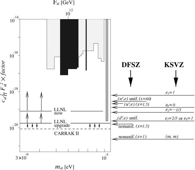
FIG. 6.: A part of Fig. 5 compared with several invisible axion models.

- [1] J. E. Kim, Phys. Rep. 150, 1 (1987).
- [2] R. D. Peccei and H. R. Quinn, Phys. Rev. Lett. 38, 1440 (1977).
- [3] C. Vafa and E. Witten, Phys. Rev. Lett. 53, 535 (1983).
- [4] H. Georgi and L. Randall, Nucl. Phys.. B276, 241 (1986).
- [5] E. Witten, Phys. Lett. B149, 351 (1984).
- [6] J. E. Kim, Phys. Rev. D31, 1733 (1985).
- [7] P. Sikivie, Phys. Rev. Lett. 48, 1156 (1982).
- [8] K. Choi and J. E. Kim, Phys. Lett. B154, 393 (1985).
- [9] J. E. Kim, Phys. Lett. B207, 434 (1988); E. J. Chun, J. E. Kim and H. P. Nilles, Nucl. Phys. B370, 105 (1992); H. Georgi, J. E. Kim and H. P. Nilles, in preparation.
- [10] J. E. Kim, Phys.. Rev. Lett. 43, 103 (1979); M. A. Shifman, A. I. Vainstein and V. I. Zakharov, Nucl. Phys. B166, 493 (1980).
- [11] H. Lewtwyler, Phys. Lett. B374, 163 (1996); K. Choi, Nucl. Phys. B383, 58 (1992).
- [12] M. Dine, W. Fischler and M. Srednicki, Phys. Lett. B104, 199 (1981); A. P. Zhitnitskii, Sov. J. Nucl. Phys. 31, 260 (1980).
- [13] P. Sikivie, Phys. Rev. Lett. 51, 1415 (1983).
- [14] D. Kaplan, Nucl. Phys. B260, 215 (1985); M. Srednicki, Nucl. Phys. B260, 689 (1985).
- [15] J. E. Kim, Harvard Univ. preprint HUTP–98/A009 (hep-ph/9802220), to appear in Phys. Rev. D.
- [16] M. S. Turner, Phys. Rep. 197, 67 (1990); G. Raffelt, Phys. Rep. 198, 1 (1990).
- [17] N. Iwamoto, Phys. Rev. Lett. 53, 1198 (1984); A. Pantziris and K. Kang, Phys. Rev. D33, 3509 (1986).
- [18] G. Raffelt and D. Seckel, Phys. Rev. Lett. 60, 1793 (1988); M. S. Turner, Phys. Rev. Lett. 60, 1797 (1988).
- [19] K. Choi, J. E. Kim and K. Kang, Phys. Rev. Lett. 62, 849 (1989).
- [20] H.-T. Janka, W. Keil, G. Raffelt, and D. Seckel, Phys. Rev. Lett. 76, 2621 (1996).
- [21] J. Ellis, J. E. Kim and D. V. Nanopoulos, Phys. Lett. B145, 181 (1984).
- [22] J. Preskill, M. B. Wise and F. Wilczek, Phys. Lett. B120, 127 (1983); L. F. Abbott and P. Sikivie, Phys. Lett. B120, 133 (1983); M. Dine and W. Fischler, Phys. Lett. B120, 137 (1983).
- [23] See, for example, M. S. Turner, Phys. Rev. D33, 889 (1986).
- [24] R. A. Battye and E. P. S. Shellard, preprint astro-ph/9706014. See also, R. L. Davis, Phys. Lett. B180, 225 (1986).
- [25] D. Harari and P. Sikivie, Phys. Lett. B195, 361 (1987).
- [26] M. Nagasawa and M. Kawasaki, Phys. Rev. D50, 4821 (1994); M. Nagasawa, Prog. Theor. Phys. 98, 851 (1997).
- [27] M. Minowa, Y. Inoue and T. Asanuma, Phys. Rev. Lett. 71, 4120 (1993)..
- [28] S. DePanfilis et al., Phys. Rev. Lett. 59, 839 (1987); C. Hagmann et al., Phys. Rev. D42, 1297 (1990).
- [29] K. van Bibber et al., Int. J. Mod. Phys. Suppl. 3, 33 (1994); C. Hagmann et al., Nucl. Phys. (Proc. Suppl.) B51, 1415 (1996).
- [30] I. Ogawa, S. Matsuki and K. Yamamoto, Phys. Rev. D53, 1740 (1996).