[

Is The Universe Infinite Or Is It Just Really Big?

Abstract

The global geometry of the universe is in principle as observable an attribute as local curvature. Previous studies have established that if the universe is wrapped into a flat hypertorus, the simplest compact space, then the fundamental domain must be at least $0.4$ times the diameter of the observable universe. Despite a standard lore that the other five compact, orientable flat spaces are more weakly constrained, we find the same bound holds for all. Our analysis provides the first limits on compact cosmologies built from the identifications of hexagonal prisms.

]

Our universe appears to stretch at least ten billion light years across. As far as the eye can see, there is no visible bound to spacetime. Still the universe may not be infinite. It may be more natural for space to be topologically compact and multiconnected. There was once a cultural prejudice that the Earth was flat and unconnected, so much so that explorers were feared to have fallen off the edge. The assumption that space must be infinite may represent a similar bias. Just as most have realized that our planet is compact, we may someday learn that the entire universe is likewise compact and connected.

Interest in compact universes[1, 2, 3, 4, 5, 6] has spawned several approaches to the search for global topology. In this letter we analyze temperature fluctuations in the cosmic background radiation (CBR) for all six compact, orientable flat topologies. The simplest compact flat space, the hypertorus, was studied in Ref. [2]. Long-wavelength fluctuations could not fit inside a small torus. The resultant cutoff in the spectrum of fluctuations was used to bound the topology scale. We show that all six orientable, compact, flat spaces are cutoff at the same wavelength as the hypertorus. Since the observed quadrupole is in fact low, this alone does not lead to a particularly severe bound. Minimizing the variance of the angular power spectrum with respect to the COBE data, we maintain the conservative conclusion that if the universe is finite and flat, it is bigger than 40% of the diameter of the surface of last scatter. The physical universe is then $\geq 2400{(H_{o}/100{\rm km/s/Mpc})}^{-1}$ Mpc across. Note that there could still be as many as eight copies of our cosmos within the observable horizon.

Tiny ripples in the gravitational potential $\Phi$ induce temperature fluctuations in the CBR via the Sachs-Wolfe effect

$${\delta T\over T}(\hat{n})={1\over 3}\Phi(\Delta\eta\hat{n})$$ (1)

where $\Delta\eta$ is the conformal time between today and the time of decoupling. The potential can be decomposed into eigenmodes ${\Phi}=\int_{-\infty}^{\infty}d^{3}\vec{k}\hat{\Phi}_{\vec{k}}\exp\left(i\Delta\eta{\vec{k}}\cdot\hat{n}\right)$. The $\hat{\Phi}_{\vec{k}}$ are primordially seeded Gaussian amplitudes that obey the reality condition $\hat{\Phi}_{\vec{k}}=\hat{\Phi}_{-\vec{k}}^{*}$. On a compact manifold, the continuous spectrum of eigenvalues, $\vec{k}$, becomes discretized. In general we write the temperature fluctuation in any compact, flat spacetime as

$\displaystyle{\delta T\over T}(\hat{n})\propto\sum_{-\infty<k_{x},k_{y},k_{z}<\infty}\hat{\Phi}_{jwn}\exp\left(i\Delta\eta\vec{k}\cdot\hat{n}\right),$

up to a normalization. As a result of the global topology, all of these spaces are anisotropic and all except for the hypertorus are inhomogeneous.

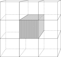
FIG. 1.: Tiling flat space with parallelepipeds.

Three dimensional Euclidean space can be made topologically compact by beginning with either a parallelepiped or a hexagonal prism as the finite fundamental domain. Six different orientable, compact spaces can be constructed by gluing opposite faces of the fundamental polyhedron. Another way to represent the identifications is to tile space with copies of the fundamental domain as shown in Figs. 1 and 3. There are four compact, orientable spaces that can be constructed from the parallelepiped tiling and two from the hexagonal tiling. The hypertorus is the simplest and is built out of a parallelepiped by identifying $x\rightarrow x+h$, $y\rightarrow y+b$ and $z\rightarrow z+c$. The identification leads to a restriction of the eigenvalue spectrum,

$$k_{x}={2\pi\over h}j\quad\quad k_{y}={2\pi\over b}w\quad\quad k_{z}={2\pi\over c}n\ \$$ (2)

with the $j,w,n$ running over all integers. It is clear that there is a minimum eigenvalue and hence a maximum wavelength which can fit inside the fundamental domain defined by the parallelepiped [2]:

$\displaystyle k_{\rm min}=2\pi\ {\rm min}\left({1\over h},{1\over b},{1\over c}\right)\quad{\lambda}_{\rm max}={\rm max}\left(h,b,c\right)\ .$

The incompatibility between this truncated angular power spectrum and a standard flat spectrum means the width of a square hypertorus had to be $0.8$ the radius of the surface of last scatter or $0.4$ of the diameter.

Three other spacetimes involve the identification of opposite sides of the parallelepiped with one or more of the faces twisted before being affixed to its counterpart. It was argued that with these twists, longer wavelengths could fit in the fundamental domain since a wave needs to wrap more than once before coming back to a fully periodic identification. However, we find upon closer inspection that these long modes are forbidden and all the compact topologies have the same cutoff as the hypertorus.

The first twisted parallelepiped we consider has opposite faces identified with one pair rotated through the angle $\pi$. The periodicity condition requires $\Phi(x,y,z)=\Phi(-x,-y,z+c)=\Phi(x,y,z+2c)$. A translation through $\Delta z=2c$ enforces

$${\Phi}(x,y,z) \equiv \int_{-\infty}^{\infty}\ d^{3}\vec{k}\ \hat{\Phi}_{\vec{k}}\ e^{i{\vec{k}}\cdot\vec{x}}$$ (3)

$$= \int_{-\infty}^{\infty}\ d^{3}\vec{k}\ \hat{\Phi}_{\vec{k}}\ e^{i{\vec{k}}\cdot\vec{x}}e^{ik_{z}2c}$$ (4)

$$= \Phi(x,y,z+2c)\ \ .$$ (5)

Matching coefficients, it follows that $e^{ik_{z}2c}=1$. With the remaining two faces identified without any twists the eigenmodes are

$$k_{x}={2\pi\over h}j\quad\quad k_{y}={2\pi\over b}w\quad\quad k_{z}={\pi\over c}n\ \ .$$ (6)

At first glance it appears as though a long mode of wavelength $2c$ fits inside the twisted space, but this eigenmode is disallowed. A translation only once through to $\Delta z=c$ requires $\Phi(x,y,z)=\Phi(-x,-y,z+c)$ so that

$${\Phi}(x,y,z) = \sum_{-\infty}^{\infty}\ \hat{\Phi}_{jwn}\ e^{2\pi i((j/h)x+(w/b)y)}e^{i\pi(n/c)z}$$ (7)

$$= \sum_{-\infty}^{\infty}\ \hat{\Phi}_{jwn}\ e^{-2\pi i((j/h)x+(w/b)y)}e^{i\pi{n\over c}(z+c)}$$ (8)

$$= \Phi(-x,-y,z+c)\ \ .$$ (9)

Matching coefficients gives

$$\hat{\Phi}_{jwn}=\hat{\Phi}_{-j-wn}\ e^{i{\pi}n}$$ (10)

and consequently, the spectrum is not only discrete, but there is also a condition on the coefficients of the eigenmodes. As a result, the cutoff is not twice as long in the $z-$direction. If $j=w=0$, then (10) requires $n$ to be even and so the lowest mode in the $z$-direction is still $k_{z}=2\pi/c$. If all scales are set equal $j=0,$ and $w=1$, then the $n=1$ mode is allowed but its wavenumber $k=\sqrt{5}\pi/c$ which is bigger than $k_{\rm min}=2\pi/c$.

FIG. 2.: $\delta T/T_{\ell}$ in $\mu K$ for the hypertorus and the $\pi/2$-twisted space. The shaded band allows for cosmic variance. The topology scale is equal to the diameter of the sphere of last scatter with $h=2\Delta\eta$.

Another possible compact space identifies opposite faces with one face rotated by $\pi/2$. After four passes through $z$ one is returned to $(x,y,z)=(x,y,z+4c)$ while as before the other faces are identified without twists. The discrete eigenmodes are

$$k_{x}={2\pi\over h}j\quad\quad k_{y}={2\pi\over h}w\quad\quad k_{z}={\pi\over 2c}n\ \ .$$ (11)

The width of the fundamental domain along $y$ must equal that along $x$. The translations along $z$ through $c,2c,$ and $3c$ result in the following restrictions:

$$\hat{\Phi}_{jwn} = \hat{\Phi}_{w-jn}e^{in\pi/2}$$ (12)

$$= \hat{\Phi}_{-w-jn}e^{in\pi}$$ (13)

$$= \hat{\Phi}_{-wjn}e^{i3n\pi/2}\ \ .$$ (14)

Again, when $j=w=0$, then $n=4m$ and the lowest eigenmode has $k_{z}=2\pi/c$ for an equal sided parallelepiped. Notice also that $\hat{\Phi}_{01n}=\hat{\Phi}_{10n}=0$. The $j=w=n=1$ mode is allowed and, setting all topology scales equal, $k=3\pi/c$ which is a smaller wavelength. Statistics that average over the sky, such as the angular power spectrum, will locate a cutoff at roughly the same mode as for the torus.

The last parallelepiped is a bit more intricate to build. The identifications are as follows [7]: Translate along $x$ and then rotate around $x$ by $\pi$ so that $(x,y,z)\rightarrow(x+h,-y,-z)$. Next, translate along $y$ and $z$, then rotate around $y$ by $\pi$ so that $(x,y,z)\rightarrow(-x,y+b,-(z+c))$. Finally, translate along $x,y$ and $z$, then rotate around $z$ by $\pi$ so that $(x,y,z)\rightarrow(-(x+h),-(y+b),z+c)$. The discrete spectrum is

$$k_{x}={\pi\over h}j\quad\quad k_{y}={\pi\over b}w\quad\quad k_{z}={\pi\over c}n\ \ ,$$ (15)

with the restricted coefficients

$$\hat{\Phi}_{jwn} = \hat{\Phi}_{j-w-n}\ e^{i\pi j}$$ (16)

$$= \hat{\Phi}_{-jw-n}\ e^{i\pi(w+n)}$$ (17)

$$= \hat{\Phi}_{-j-wn}\ e^{i\pi(j+w+n)}\ \ .$$ (18)

No permutations of $(0,0,1)$ are allowed although $(0,1,1)$ permutations are accessible, although with fixed phases with repect to the fundamental domain.

Spectra for the hypertorus and the $\pi/2$-twisted parallelepiped, both as big as the observable universe, are shown in Fig. 2. The power spectrum is defined as usual: $C_{\ell}=\sum_{m}|a_{\ell m}|^{2}/(2\ell+1)$ with the $a_{\ell m}$ defined by the decomposition of the temperature anisotropy into spherical harmonics, $\delta T/T=\sum_{\ell m}a_{\ell m}Y_{\ell m}$. For convenience we plot the quantity ${\delta T/T}_{\ell}=\left[\ell(\ell+1)C_{\ell}/2\pi\right]^{1/2}$ measured in $\mu K$ and compare the model values with the COBE data as analyzed by Gorski (diamonds) [8], by Tegmark (open circles) [9], and by Bond, Jaffe and Knox (filled circles) [10]. While small universes can be ruled out, it is rather fascinating to note that these large cases are marginally consistent with the data. After all, the observed quadrupole is low. It is also not possible to tell if the observed power spectrum is a smooth function or a sparcely sampled jagged function.

The hexagonal tiling of flat space gives two new topologies. (It is curious to note that flat space can also be tiled with fractal hexagons [11].) Three pairs of opposite sides of the hexagon are identified while in the $z$ direction, the faces are rotated relative to each other by $2\pi/3$. The potential can be written as

$$\Phi= \sum_{n_{2}n_{3}n_{z}} \hat{\Phi}_{n_{2}n_{3}n_{z}}e^{ik_{z}n_{z}}\times$$ (19)

$$\exp {\left[i{2\pi\over h}\left[n_{2}\left(-x+{1\over\sqrt{3}}y\right)+n_{3}\left(x+{1\over\sqrt{3}}y\right)\right]\right]}$$ (20)

with the eigenmodes

$$k_{x}={2\pi\over h}j\quad\quad k_{y}={2\pi\over h}w\quad\quad k_{z}={2\pi\over 3c}{n_{z}}$$ (21)

and

$$\hat{\Phi}_{n_{2},n_{3},n_{z}} = \hat{\Phi}_{n_{3},-(n_{2}+n_{3}),n_{z}}e^{i2\pi n_{z}/3}$$ (22)

$$= \hat{\Phi}_{-(n_{2}+n_{3}),n_{3},n_{z}}e^{i4\pi n_{z}/3}\ \ .$$ (23)

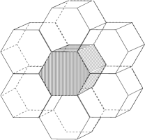
FIG. 3.: Tiling flat space with hexagonal prisms.

The last possibility for 3D Euclidean spaces identifies the $z$-faces after rotation by $\pi/3$. The potential can still be written as (19) with

$$k_{x}={2\pi\over h}j\quad\quad k_{y}={2\pi\over h}w\quad\quad k_{z}={\pi\over 3c}{n_{z}}$$ (24)

and

$$\hat{\Phi}_{n_{2},n_{3},n_{z}} = \hat{\Phi}_{(n_{2}+n_{3}),-(n_{2}-n_{3})/\sqrt{3},n_{z}}e^{i\pi n_{z}/3}$$ (25)

$$= \hat{\Phi}_{n_{3},-(n_{2}-n_{3}),n_{z}}e^{2i\pi n_{z}/3}$$ (26)

$$= \hat{\Phi}_{-n_{2},(n_{2}-n_{3})/\sqrt{3},n_{z}}e^{i\pi n_{z}}$$ (27)

$$= \hat{\Phi}_{-(n_{2}+n_{3}),n_{3},n_{z}}e^{i4\pi n_{z}/3}\ \ .$$ (28)

For both of the hexagons the first $n_{2}=n_{3}=0$ mode has $k_{\rm min}=2\pi n_{z}/c$, as always. Spectra for the hexagonal prisms the size of the observable universe are shown in Fig. 4. Again, they are all consistent with the data.

FIG. 4.: ${\delta T/T}_{\ell}$ in $\mu K$ for the 2 spaces build from a hexagonal prism fundamental domain. The topology scale is comparable the diameter of the sphere of last scatter with $h=2\Delta\eta$. The shaded area accounts for cosmic variance.

In Fig. 5, sample small universe spectra are shown. As a result of the low observed quadrupole, the predicted cutoff alone is not enough to discourage compact models. We can however ask how likely the spectra shown are relative to the spectrum of a flat, infinite cosmology. Since compact topologies do not give isotropic Gaussian temperature fluctuations, we need to be cautious in making quantitative conclusions based on any likelihood method. For this reason, we have maintained the conservative bound of $h\geq 0.8\Delta\eta$ which is safely ruled out based on the likelihood analysis of Ref. [10]. The predicted spectrum is normalized to COBE by minimizing a variance in the natural logarithm of $\delta T/T_{\ell}$ and the likelihood of the spectrum is assessed given the data. Compact spaces with a topology scale of $0.8$ the radius of the last scattering surface, $0.4$ the diameter, are at best tens of times less likely than an infinite universe.

FIG. 5.: ${\delta T/T}_{\ell}$ in $\mu K$ for two small universes with $h=0.8\Delta\eta$. The leftmost figure is for a regular hypertorus twist and the rightmost is for the hexagon with a $120^{o}$ twist. Cosmic variance is included in the shaded strip.

While the angular power spectrum is sufficient to constrain symmetric, flat topology it is in general a poor discriminant. The average over the sky fails to recognize the strong inhomogeneity and anisotropy manifest in these cosmologies. Fig. 6 shows a simulated CBR map of a $\pi$-twisted compact cosmos. The topology scales relative to the radius of the last scattering surface are $h=2,b=1,c=0.5$. In the upper panel, the observer is at the origin. In the bottom map, we have offset the observer from the origin. While the ${\delta T/T}_{\ell}$ can be used to bound equal sided small universes, the characterization falters for this anisotropic example. The map on the other hand shows the markings of the geometry, and a better statistic for extracting correlations is sorely needed. The symmetry studies of Ref. [12] that place lower bounds on anisotropic hypertori hint at the power of such a pattern-oriented approach. We are currently developing more powerful and general methods to identify patterns hidden in the data [13].

Our prejudice that the universe is infinite may be no more justified than the old prejudice that the Earth is flat. The exploration of the universe for signs of topology is really just beginning. While very small flat spaces appear less likely, there are an infinite number of compact, negatively curved possibilities which remain unconstrained. The search for patterns in sky maps may be of particular importance in identifying these [13]. As our vision improves with the aid of future satellite missions, we may soon be able to see, literally see, the global geometry of our universe.

___________________________

We appreciate the valuable input from J.R. Bond, N. Cornish, P. Ferreira, K. Gorski, T. Saurodeep, D. Spergel and G. Starkman. We are indebted to Andrew Jaffe for teaching us the likelihood methods of Ref. [10]. We are also grateful to Ted Bunn for allowing us to adapt his codes. E.S. is supported by the NSF.

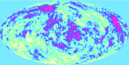
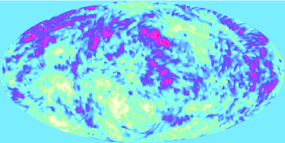
FIG. 6.: Top: a simulated map of the microwave sky for a $\pi$ twisted space with topology scales $h=2,b=1,c=0.5$. Middle: same space with the observer offset from the origin of the universe. Bottom: ${\delta T/T}_{\ell}$ for the lower map.

REFERENCES

- [1] J. Levin, J.D. Barrow, E.F. Bunn and J. Silk, Phys. Rev. Lett. 79 (1997) 974 .
- [2] D. Stevens, D. Scott and J. Silk, Phys. Rev. Lett. 71 (1993) 20.
- [3] M. Lachieze-Rey and J.P. Luminet, Phys. Rep. 254 (1995) 135; R. Lehoucq, M. Lachieze-Rey and J.P. Luminet, “Cosmic Crystallography”, gr-qc/9604050.
- [4] J.D. Barrow and J. Levin,Phys. Lett. A 233 (1997) 169.
- [5] N.J. Cornish, D. Spergel and G. Starkman, astro-ph/9602039 (1996); ibid. astro-ph/9708225 (1997).
- [6] J. R. Bond, D. Pogosyan and T. Souradeep, preprint astro-ph/9702212 (1997); ibid. in preparation.
- [7] J.A. Wolf, “Spaces of Constant Curvature” (Publish or Perish, Inc., Wilmington, Delaware, 1967).
- [8] K. Gorski, Proc. Moriond XVI, ed. F.R. Bouchet et. al. (Gif-Sur-Yvette: Editions Frontièrs) (1997).
- [9] M. Tegmark Phys. Rev. D 55 (1997) 5895.
- [10] J.R. Bond, A. Jaffe and L. Knox, preprint CfPA-97-TH-11; ibid. in preparation; J.R. Bond and A. Jaffe, Proc. Moriond XVI, ed. F.R. Bouchet et. al. (Gif-Sur-Yvette: Editions Frontièrs) (1997).
- [11] Schröder, Chaos, Fractals and Power Laws (W.H.Freeman and Company, 1991).
- [12] A. de Oliveira-Costa and G. F. Smoot, Ap.J. 448 (1995) 447; A. de Oliveira-Costa, G. F. Smoot, and A. A. Starobinsky, Ap. J. 468 (1996) 457.
- [13] J. Levin, E. Scannapieco, J. Silk and J.D. Barrow, “How the Universe Got Its Spots”, in preparation.