Sonderforschungsbereich 375 $\bullet$ Research in Particle-Astrophysics

Technische Universität München (TUM) $\cdot$ Ludwig-Maximilians-Universität München (LMU)

Max-Planck-Institut für Physik (MPP) $\cdot$ Max-Planck-Institut für Astrophysik (MPA)

Proceedings of the Fourth SFB-375 Ringberg Workshop

Neutrino Astrophysics

Ringberg Castle, Tegernsee, Germany

October 20–24, 1997

Program Committee:	Michael Altmann, Wolfgang Hillebrandt, Hans-Thomas Janka,
	Manfred Lindner, Lothar Oberauer, Georg Raffelt

edited by

Michael Altmann, Wolfgang Hillebrandt, Hans-Thomas Janka and Georg Raffelt

January 1998

Proceedings of the Fourth SFB-375 Ringberg Workshop “Neutrino Astrophysics”

Sonderforschungsbereich 375 Research in Astro-Particle Physics
E-mail: depner@e15.physik.tu-muenchen.de

Postal Address:

Technische Universität München
Physik Department E15 — SFB–375
James-Franck-Straße
D–85747 Garching
Germany

© Sonderforschungsbereich 375 and individual contributors

Published by the Sonderforschungsbereich 375
Technische Universität München, D–85747 Garching
January 1998

Preface

This was the fourth workshop in our series of annual “retreats” of the Sonderforschungsbereich Astroteilchenphysik (Special Research Center for Astroparticle Physics), or SFB for short, to the Ringberg Castle above Lake Tegernsee in the foothills of the Alps. These meetings are meant to bring together the members of the SFB which are dispersed between four institutions in the Munich area, the Technical University Munich (TUM), the Ludwig-Maximilians-University (LMU), and the Max-Planck-Institute for Physics (MPP) and that for Astrophysics (MPA). We always invite a number of external speakers, including visitors at our institutions, to complement the scientific program and to further the exchange of ideas with the international community.

This year’s topic was “Neutrino Astrophysics” which undoubtedly is one of the central pillars of astroparticle physics. We focused on the astrophysical and observational aspects of this field, deliberately leaving out theoretical particle physics and laboratory experiments from the agenda. Each day of the workshop was dedicated to a specific sub-topic, ranging from solar, supernova and atmospheric neutrinos over high-energy cosmic rays to the early universe. A session on future prospects served to conclude the workshop and provide an outlook on the field in the next decade and beyond. We started every topical session with one or two introductory talks, reviewing the status of theory and experiment and to providing some background for the non-experts.

For the entire program we interpreted “neutrino astrophysics” in a broad sense, including, for example, the physics of $\gamma$-ray bursts or the recent observations of TeV $\gamma$-rays by the imaging air-Cherenkov technique. Some of the after-dinner-talks went significantly beyond a narrow interpretation of the field! From our perspective the profile of neutrino astrophysics as defined by our program worked very well, even better than we had hoped. We are proud that the main complaint of the participants seemed to be that they did not get enough mountain-hiking done because the sessions were too interesting to miss.

Besides regular SFB resources this workshop was made possible by a direct grant from the Max-Planck-Society and additional funds from the Max-Planck-Institute for Astrophysics. Special thanks go to the SFB secretary, Maria Depner, for her smooth and skillful management of all practical matters related to the workshop.

We thank the participants for their high-level contributions and for being extremely co-operative in submitting the “extended abstracts” of their talks on time and in a format that allowed us to produce these proceedings in electronic form. Anyone interested in a printed version should write to the SFB secretary at the address given on the previous page. We hope that you will find this booklet a useful and up-to-date resource for the exciting and fast-developing field of neutrino astrophysics.

Michael Altmann, Wolfgang Hillebrandt, Hans-Thomas Janka and Georg Raffelt

Munich, January 1998

Contents

History

R.L. Mößbauer
     History of Neutrino Physics: Pauli’s Letters  3

A. Dar
     What Killed the Dinosaurs?  6

Solar Neutrinos

M. Stix
     Solar Models  13

H. Schlattl, A. Weiss
     Garching Solar Model: Present Status  19

M. Altmann
     Status of the Radiochemical Gallium Solar Neutrino Experiments  22

Y. Fukuda (for the Superkamiokande Collaboration)
     Solar Neutrino Observation with Superkamiokande  26

M.E. Moorhead (for the SNO Collaboration)
     The Sudbury Neutrino Observatory  31

L. Oberauer (for the Borexino Collaboration)
     BOREXINO  33

M. Junker (for the LUNA Collaboration)
     Measurements of Low Energy Nuclear Cross Sections  36

G. Fiorentini
     Solar Neutrinos: Where We Are and What Is Next?  40

Supernova Neutrinos

W. Hillebrandt
     Phenomenology of Supernova Explosions  47

B. Leibundgut
     Supernova Rates  51

A.G. Lyne
     Pulsar Velocities and Their Implications  54

W. Keil
     Convection in Newly Born Neutron Stars  57

H.-Th. Janka
     Anisotropic Supernovae, Magnetic Fields, and Neutron Star Kicks  60

K. Sato, T. Totani, Y. Yoshii
     Spectrum of the Supernova Relic Neutrino Background and Evolution of Galaxies  66

G.G. Raffelt
     Supernova Neutrino Opacities  73

S.J. Hardy
     Quasilinear Diffusion of Neutrinos in Plasma  75

P. Elmfors
     Anisotropic Neutrino Propagation in a Magnetized Plasma  79

A.N. Ioannisian, G.G. Raffelt
     Cherenkov Radiation by Massless Neutrinos in a Magnetic Field  83

A. Kopf
     Photon Dispersion in a Supernova Core  86

Gamma-Ray Bursts

D.H. Hartmann, D.L. Band
     Gamma-Ray Burst Observations  91

S.E. Woosley, A. MacFadyen
     Gamma-Ray Bursts: Models That Don’t Work and Some That Might  96

M. Ruffert, H.-Th. Janka
     Models of Coalescing Neutron Stars with Different Masses and Impact Parameters  101

R.A. Sunyaev
     Physical Processes Near Black Holes  106

High-Energy Neutrinos

K. Mannheim
     Astrophysical Sources of High -Energy Neutrinos  109

P. Gondolo
     Atmospheric Muons and Neutrinos Above 1 TeV  112

D. Kiełczewska
     Atmospheric Neutrinos in Super-Kamiokande  116

Ch. Wiebusch
     Neutrino Astronomy with AMANDA  121

M.E. Moorhead
     High Energy Neutrino Astronomy with ANTARES  127

R. Plaga
     Ground-Based Observation of Gamma-Rays (200 GeV–100 TeV)  130

Cosmology

C.J. Hogan
     Helium Absorption and Cosmic Reionization  139

K. Jedamzik
     Non-Standard Big Bang Nucleosynthesis Scenarios  141

J.B. Rehm, K. Jedamzik
     Big Bang Nucleosynthesis With Small-Scale Matter-Antimatter Domains  147

M. Bartelmann
     Neutrinos and Structure Formation in the Universe  149

Future Prospects

P. Meunier
     Neutrino Experiments with Cryogenic Detectors  161

P.F. Smith
     OMNIS—A Galactic Supernova Observatory  165

J. Valle
     Neutrinos in Astrophysics  170

L. Stodolsky
     Some Neutrino Events of the 21st Century  178

Appendix

Workshop Program and List of Participants  183

Our Sonderforschungsbereich (SFB) “Astro-Teilchen-Physik” and its Divisions  193

History

History of Neutrino Physics: Pauli’s Letters

Rudolf L. Mößbauer

Physik Department E15, Technische Universität München, 85747 Garching, Germany

Editors’ Note

Professor Mößbauer gave an evening lecture on the history of neutrino physics during which he read Pauli’s famous letters on the neutrino hypothesis. Rather than writing a formal contribution to our proceedings, Professor Mößbauer suggested that we reproduce these letters. (They were taken from Ref. [1] but can also be found in Ref. [2].) Because much of the humour of Pauli’s writing is lost in the translation we quote the original German text. An English translation can be found, for example, in Ref. [3].

Figure 1: Wolfgang Pauli (1900–1958) in Vienna 1933.

Pauli’s Letters

Brief an Oskar Klein, Stockholm, vom 18. 2. 1929

Aber ich verstehe zu wenig von Experimentalphysik um diese Ansicht beweisen zu können und so ist Bohr in der für ihn angenehmen Lage, unter Ausnutzung meiner allgemeinen Hilflosigkeit bei der Diskussion von Experimenten sich selber und mir unter Berufung auf Cambridger Autoritäten (übrigens ohne Literaturangabe) da etwas beliebiges vormachen zu können.

Brief an Oskar Klein, Stockholm, 1929

Ich selbst bin ziemlich sicher (Heisenberg nicht so unbedingt), daß $\gamma$-Strahlen die Ursache des kontinuierlichen Spektrums der $\beta$-Strahlen sein müssen und daß  Bohr mit seinen diesbezüglichen Betrachtungen über eine Verletzung des Energiesatzes auf vollkommen falscher Fährte ist. Auch glaube ich, daß  die wärmemessenden Experimentatoren irgendwie dabei mogeln und die $\gamma$-Strahlen ihnen nur infolge ihrer Ungeschicklichkeit bisher entgangen sind.

Brief an die Gruppe der “Radioaktiven” 1930

Physikalisches Institut
der Eidg. Technischen Hochschule
Zürich Zürich, 4. Dez. 1930

Liebe Radioaktive Damen und Herren!
Wie der Überbringer dieser Zeilen, den ich huldvollst anzuhören bitte, Ihnen des näheren auseinandersetzen wird, bin ich angesichts der falschen Statistik der N- und Li 6-Kerne, sowie des kontinuierlichen $\beta$-Spektrums auf einen verzweifelten Ausweg verfallen, um den Wechselsatz der Statistik und den Energiesatz zu retten. Nämlich die Möglichkeit, es könnten elektrisch neutrale Teilchen, die ich Neutronen nennen will, in den Kernen existieren, welche den Spin 1/2 haben und das Ausschließungsprinzip befolgen und sich von Lichtquanten außerdem noch dadurch unterscheiden, daß sie nicht mit Lichtgeschwindigkeit laufen. — Das kontinuierliche $\beta$-Spektrum wäre dann verständlich unter der Annahme, daß  beim $\beta$-Zerfall mit dem Elektron jeweils noch ein Neutron emittiert wird, derart, daß  die Summe der Energien von Neutron und Elektron konstant ist.

Nun handelt es sich weiter darum, welche Kräfte auf die Neutronen wirken. Das wahrscheinlichste Modell für das Neutron scheint mir aus wellenmechanischen Gründen dieses zu sein, daß  das ruhende Neutron ein magnetischer Dipol von einem gewissen Moment $\mu$ ist. Die Experimente verlangen wohl, daß  die ionisierende Wirkung eines solchen Neutrons nicht größer sein kann als die eines $\gamma$-Strahls, und dann darf $\mu$ wohl nicht größer sein als $e\cdot(10^{-13}$ cm). Ich traue mich vorläufig aber nicht, etwas über diese Idee zu publizieren, und wende mich erst vertrauensvoll an Euch, liebe Radioaktive, mit der Frage, wie es um den experimentellen Nachweis eines solchen Neutrons stände, wenn dieses ein ebensolches oder etwa 10mal größeres Durchdringungsvermögen besitzen würde wie ein $\gamma$-Strahl. $\ldots$

Also, liebe Radioaktive, prüfet, und richtet.—Leider kann ich nicht persönlich in Tübingen erscheinen, da ich infolge eines in der Nacht vom 6. zum 7. Dez. in Zürich stattfindenden Balles hier unabkömmlich bin. $\ldots$ Euer untertänigster Diener W. Pauli

Brief an Oskar Klein, Stockholm, vom 12. 12. 1930

Ich kann mich vorläufig nicht entschließen, an ein Versagen des Energiesatzes ernstlich zu glauben und zwar aus folgenden Gründen (von denen ich natürlich zugebe, daß sie nicht absolut zwingend sind). Erstens scheint es mir daß der Erhaltungssatz für Energie-Impuls dem für die Ladung doch sehr weitgehend analog ist und kann keinen theoretischen Grund dafür sehen, warum letzterer noch gelten sollte (wie wir es ja empirisch über den $\beta$-Zerfall wissen) wenn ersterer versagt. Zweitens müßte bei einer Verletzung des Energiesatzes auch mit dem Gewicht etwas sehr merkwürdiges passieren.

Telegramm von Reines und Cowan vom 14. 6. 1957 an Wolfgang Pauli

We are happy to inform you that we have definitely detected neutrinos from fission fragments by observing inverse beta decay of protons. Observed cross section agrees well with expected $6\cdot 10^{-44}$ cm².

What Killed The Dinosaurs?

Arnon Dar<sup>1,2

1</sup>Max-Planck-Institut für Physik (Werner-Heisenberg-Institut)
Föhringer Ring 6, 80805 München, Germany.
²Department of Physics and Space Research Institute,
Technion, Israel Institute of Technology, Haifa 32000, Israel.

The early history of life during the Precambrian until its end 570 million years (My) ago is poorly known. Since then the diversity of both marine and continental life has increased exponentially. Analysis of fossil records shows that this diversification was interrupted by five massive extinctions and some smaller extinction peaks [1]. The largest extinction occurred about 251 My ago at the end of the Permian period. The global species extinction ranged then between 80% to 95%, much more than, for instance, the Cretaceous-Tertiary extinction 64 My ago which killed the dinosaurs and claimed $\sim 47\%$ of existing genera [2]. In spite of intensive studies it is still not known what caused the mass extinctions. Many extinction mechanisms have been proposed but no single mechanism seems to provide a satisfactory explanation of the complex geological records on mass extinctions [3]. These include terrestrial mechanisms such as intense volcanism, which coincided only with two major extinctions [4] or drastic changes in sea level, climate and environment that occurred too often, and astrophysical mechanisms, such as a meteoritic impact that explains the iridium anomaly which was found at the Cretaceous/Tertiary boundary [5] but has not been found in any of the other extinctions, supernova explosions [6] and gamma ray bursts [7] which do not occur close enough at a sufficiently high rate to explain the observed rate of mass extinctions.

The geological records, however, seem to indicate that an accidental combination of drastic events [3] occurred around the times of the major extinctions. For instance, the dinosaur extinction coincides in time with a large meteoritic impact, with a most intensive volcanic eruption and with a drastic change in sea level and climate. The origin of these correlations is still unclear. Meteoritic impacts alone or volcano eruptions alone or sea regression alone could not have caused all the major mass extinctions. An impact of a 10 km wide meteorite with a typical velocity of $30~{}\rm km~{}s^{-1}$ was invoked [5] in order to explain the Cretaceous-Tertiary (K/T) mass extinction 64 My ago, which killed the dinosaurs, and the iridium anomaly observed at the K/T boundary. But neither an iridium anomaly nor a large meteoritic crater have been dated back to 251 My ago, the time of the Permian/Triassic (P/T) mass extinction, which was the largest known extinction in the history of life [3] where the global species extinction ranged between 80% to 95%. The gigantic Deccan volcanism in India that occurred around the K/T boundary [4] and the gigantic Siberian basalts flood that occurred around the P/T boundary have ejected approximately $2\times 10^{6}~{}\rm km^{3}$ of lava [4]. They were more than a thousand times larger than any other known eruption on Earth, making it unlikely that the other major mass extinctions, which are of a similar magnitude, were produced by volcanic eruptions. Although there is no one-to-one correspondence between major mass extinctions, large volcanic eruptions, large meteoritic impacts, and drastic environmental changes, there are clear time correlations between them. We propose that near encounters of Earth with “visiting planets” from the outer solar system are responsible for most of the mass extinctions on planet Earth and can explain both the above correlations and the detailed geological records on mass extinctions [8].

Recent observations with the Hubble Space Telescope of the Helix Nebula (Fig. 1) the nearest planetary nebula, have discovered [9] that the central star is surrounded by a circumstellar ring of about 3500 gigantic comet-like objects (“Cometary Knots”) with typical masses about $10^{-5}M_{\odot}$, comparable to our solar system planets ($M_{\rm Earth}\approx 3\times 10^{-6}M_{\odot}$ and $M_{\rm Jupiter}\approx 9.6\times 10^{-4}M_{\odot}$). It is not clear whether they contain a solid body or uncollapsed gas. They are observed at distances comparable to our own Oort cloud of comets but they seem to be distributed in a planar ring rather than in a spherical cloud like the Oort cloud. It is possible that these Cometary Knots have been formed together with the central star since star formation commonly involves formation of a thin planar disk of material possessing too high an angular momentum to be drawn into the nascent star and a much thicker outer ring of material extending out to several hundred AU. Evidence for this material has been provided by infrared photometry of young stars and also by direct imaging.

It is possible that such Cometary Knots and the recently discovered gigantic asteroids [10] in the outer solar system between the Kuiper belt and the Oort cloud are the high mass end of the vastly more numerous low mass comets. The massive objects are more confined to the ecliptic plane because of their relatively large masses, and form a circumstellar ring, while the very light ones are scattered by gravitational collisions into a spherical Oort cloud. Gravitational interactions in the ring can change their parking orbits into orbits which may bring them into the inner solar system. In fact, various “anomalies” in the solar planetary system [11] could have resulted from collisions or near encounters with such visitors in the early solar system. These include [12] the formation of the moon, the large eccentricity and inclination of some planetary orbits, the retrograde orbits of 6 moons of Jupiter, Uranus and Neptune and the tilted spin planes of the Sun, the planets and moons relative to their orbiting plane.

Strong gravitational tidal forces can cause frictional heating of planetary interiors leading to strong volcanic activity, as seen, for instance, on Jupiter’s moon Io, the most volcanically active object known in the solar system. The moon, the Sun and the known planets are too far away to induce volcanic eruptions on Earth, but relatively recent “visits” of planet-like objects near Earth could have generated gigantic tidal waves, large volcanic eruptions, drastic changes in climate and sea level, and impacts of meteorites which were diverted into a collision course with Earth by the passage through the astroids and Kuiper belts [13]. Thus, visiting planets may provide a common origin for the diverse mass extinction patterns as documented in the geological records.

Although exact calculations of surface tidal effects are a formidable scientific effort that was begun by Newton and has continued and improved since then by many of the great mathematicians and physicists, an approximate estimate of the flexing ($h$) of Earth (radius $R_{E}$) by a passing planet (distance $d$) can be easily obtained by neglecting the rotation of Earth and the speed of the passing planet (mass $M_{p}$) and by assuming quasi hydrostatic equilibrium:

$$h\approx{3\over 4}{M_{p}\over M_{E}}\left({R_{E}\over d}\right)^{3}R_{E}.$$ (1)

The maximal crustal tide due to the moon is 27 cm. However, a visiting planet with a typical mass like that of the Cometary Knots [9] which passes near Earth at a distance comparable to the Earth-Moon distance produces gigantic oceanic and crustal tidal waves which are a few hundred times higher than those induced by the moon. Oceanic tidal waves, more than 1 km high, can flood vast areas of continental land and devastate sea life and land life near continental coasts. The spread of ocean waters by the giant tidal wave over vast areas of land and near the polar caps will enhance glaciation and sea regression.

Flexing the Earth by $h\sim 100$ m will deposit in it $\sim\alpha GM_{E}^{2}h/R_{E}^{2}\approx 10^{34}$ ergs, where $\alpha\sim 0.1$ is a geometrical factor. It is approximately the heat release within Earth during $10^{6}$ y by radioactive decays. The flexing of Earth and the release of such a large energy in a very short time upon contraction might have triggered the gigantic volcanic eruptions that produced the Siberian basalts flood at the time of the P/T extinction and the Deccan basalts flood at the time of the K/T extinction.

A reliable estimate of the masses and the flux of the visiting planets/planetesimals is not possible yet. However, we have fixed them from the assumption that the unaccounted energy source of Jupiter and its tilted spin plane relative to its orbital plane are both due to accretion of visiting planets/moons. From the $3.13^{\circ}$ tilt of Jupiter’s spin and the accretion rate, we inferred that $N_{J}\approx 16$ planets of average mass $M_{p}\approx 0.5M_{E}$ have crashed into Jupiter during its $\sim 4.57$ Gy lifetime. Similar estimates for other planets, although yielding the correct order of magnitude, are less reliable because the inferred number of accreted planets is too small. The $7^{\circ}$ tilt of the spin of the Sun could have been produced by the impact of $\sim 3\times 10^{4}$ such planets (ignoring possible angular momentum loss by the solar wind). This means that the Sun has accreted $\sim 5\%$ of its mass after its formation, at a rate of $\sim 7$ planets per My. In each capture episode, $\sim 6\times 10^{42}$ erg of gravitational energy is released in the Sun’s convective layer. It produces optical and x-ray flashes at a rate $\sim 7~{}\times 10^{-6}~{}L_{\odot}^{-1}{\rm y}^{-1}$ for Sun-like stars. It also causes a significant luminosity rise for an extended time which may have induced climatic and sea level changes on Earth, and extinctions of species which could not have adapted to large environmental changes. The predicted rate is consistent with the observed rate of large changes in O¹⁸ concentration in sea water sediments which record large changes in sea water level and total glacier volume.

Using our inferred planet flux from Jupiter and its collimation by the Sun, we obtained that a “visiting rate” of once every $t_{v}=100$ My for planets with $M_{p}\sim 0.5M_{E}$ which fall towards the Sun implies a passing distance of approximately 170,000 km from Earth which produces crustal tidal waves of $h\geq 125$ m and water tidal waves of $\sim 1~{}\rm km$ height. The combination of tidal waves, volcanic eruptions, meteoritic impacts and environmental and climatological changes can explain quite naturally the biological and time patterns of mass extinctions. For instance, the giant tidal waves devastate life in the upper oceans layers and on low lands near coastal lines. They cover large land areas with sea water, spread marine life to dry on land after water withdrawal, and sweep land life into the sea. They flood sweet water lakes and rivers with salt water and erode the continental shores where most sea bed marine life is concentrated. Amphibians, birds and inland species can probably survive the ocean tide. This may explain their survival after the K/T extinction. Survival at high altitude inland sites may explain the survival of some inland dinosaurs beyond the K/T border. Volcanic eruptions block sunlight, deplete the ozone layer, and poison the atmosphere and the sea with acid rain. Drastic sea level, climatic and environmental changes inflict further delayed blows to marine and continental life. But high-land life in fresh water rivers which are fed by springs, that is not so sensitive to temperature and climatic conditions, has better chances to survive the tidal waves, the volcano poisoning of sea water, and the drastic sea level, environmental and climatic changes.

Altogether, visiting planets offer a simple and testable solution to the puzzling correlations between mass extinctions, meteoritic impacts, volcanic eruptions, sea regression and climatic changes, as documented in the geological records. Perhaps the best test will come from the MACHO sample of $\sim$100,000 light curves of variable stars: Planets/moons crashing onto stars produce a big flash of light and soft x-rays from the hot spot at the impact point on main sequence (rotating) stars, a nova-like thermonuclear explosion on the surface of a white dwarf (rare), or a strong gamma ray flash from the surface of a neutron star (very rare).

Figure 1: A small section of a distant ring of gigantic comet-like objects around the central star in the Helix nebula, the nearest planetary nebula, as seen recently by the Hubble Space Telescope [9]. These objects have a typical mass of $5M_{E}$. Their gaseous heads have a typical size of $10^{15}$ cm. It is not clear whether they contain a solid body or uncollapsed gas.

Acknowledgements

It is a pleasure to thank the organizers of the workshop for their kind invitation and for an excellent and enjoyable meeting. Very exciting and useful discussions with P. Gondolo, G. Raffelt and L. Stodolsky during and after lunches at MPP, München, are greatfully acknowledged.

Solar Models

M. Stix

Kiepenheuer-Institut für Sonnenphysik, Freiburg, Germany

Introduction

A number of solar model calculations has been presented in recent years, especially in view of the predicted flux of neutrinos from the Sun [4, 5, 6, 9, 12, 20, 27]. In the present contribution I shall discuss mostly the Standard Solar Model. This model, including some refinements, is confirmed by seismological tests. Non-standard models, on the other hand, face severe difficulties. I close with a remark on the Sun’s magnetic field in the neutrino context.

The Standard Model

The standard solar model is a gas sphere in hydrostatic equilibrium. This may seem trivial. However, some of the earliest non-standard models were based on the assumption of a very strong internal magnetic field, or of rapid rotation of the solar core; both of these assumptions violate the spherical symmetry as well as the hydrostatic equilibrium.

The input to the standard model should be to the best of our present knowledge. Let me begin with the mass, luminosity, and radius,

$$m_{\odot}=(1.989\pm 0.001)\cdot 10^{30}{\rm kg}\ ,\quad L_{\odot}=(3.845\pm 0.008)\cdot 10^{26}{\rm W}\ ,\quad r_{\odot}=(6.960\pm 0.001)\cdot 10^{8}{\rm m}\ .$$

The value given for the luminosity is from the ACRIM experiment on the Solar Maximum Mission, with the error as quoted in [15]. The radius is for the optical depth $\tau=2/3$ where the temperature is equal to the effective temperature $(L_{\odot}/4\pi\sigma r_{\odot}^{2})^{1/4}$.

The age of the Sun is found by measuring the decay of long-lived radioactive isotopes in meteorites,

$$t_{\odot}=(4.57\pm 0.05)\cdot 10^{9}{\rm years}\ .$$

Wasserburg, in an appendix to [5], gives an even smaller error; the main source of uncertainty is the not well-known state of the formation of the Sun at the time of the melting and crystallization of the meteoritic material.

a) Chemical Composition

The composition of the solar surface (and the entire perfectly mixed outer convection zone) is derived from solar spectroscopy and from meteoritic data. Recent results [16] show a slightly decreased content of the heavy elements in comparison to earlier results, e.g. [1]. For oxygen, the most abundant element after H and He, the change is $-0.06$ in the usual logarithmic scale, or $\approx-13\%$. Altogether, the ratio of the mass fractions $Z$ and $X$ of the heavy elements and hydrogen is 0.0245, instead of the earlier value 0.0267.

For helium the most accurate determination is based on helioseismology. This is because both the sound velocity and the acoustic cut-off frequency depend on the adiabatic exponent $\Gamma_{1}$:

$$c^{2}={P\Gamma_{1}\over\rho}\ ,\qquad\omega_{A}={g\Gamma_{1}\over 2c}\ ,\qquad\Gamma_{1}=\biggl{(}{d\ln T\over d\ln P}\biggr{)}_{S}\ .$$

In the depth range where an abundant element is partly ionized $\Gamma_{1}$ is greatly affected by the energy of ionization. Thus the He abundance, in particular by its effect in the zone of partial HeII ionization, has some influence on the eigenfrequencies of the Sun’s pressure (p) modes of oscillation. The inversion of observed frequencies yields a mass fraction $Y_{S}=0.242\pm 0.003$ ([22], other authors find similar results). It should be noted that the original He abundance, $Y_{0}$, is adjusted so that the luminosity of the present model, at age $t_{\odot}$, equals $L_{\odot}$. The result of this procedure is $Y_{0}=0.27\dots 0.28$, depending on other input to the model. The difference to the seismically determined $Y_{S}$ is appropriate in view of helium settling in the radiative solar interior, see below.

b) Nuclear Reactions

Concerning the nuclear reactions I shall concentrate on the pp chains, which provide $\approx 99\%$ of the energy. The reaction rates, and therefore the branching between the three chains leading to helium, depend on temperature (see below), and on the “astrophysical $S$-factor” $S(E)$. This factor depends weakly on the center-of-mass energy $E$ and measures the cross section after separation of $1/E$ times the penetration probability through the Coulomb barrier. For the most important reactions Parker [21] reviews results of $S$-factors (at zero energy):

p(p,e${}^{+}\nu$)d	$S_{11}(0)=3.89\cdot 10^{-25}$ MeV$\cdot$b	$\pm 1\%$
3He(3He,2p)4He	$S_{33}(0)=5.0$ MeV$\cdot$b	$\pm 6\%$
3He(4He,$\gamma)^{7}$Be	$S_{34}(0)=533$ eV$\cdot$b	$\pm 4\%$
7Be(p,$\gamma)^{8}$B	$S_{17}(0)=22.2$ eV$\cdot$b	$\pm 14\%$

It is difficult to assess the errors. $S_{11}$ is so small that it can only be calculated. The other $S$-factors are measured in the laboratory but must be extrapolated to zero energy, and a correction must be applied for electron screening at low energy. In particular the $14\%$ error of $S_{17}$ has been criticized, e.g. [17], as it is derived from diverse experiments with partially contradicting results in the range 17.9–27.7 eV$\cdot$b. Perhaps better results will soon become available as the measurements are extended to lower energy, cf. the contribution of M. Junker to these proceedings.

c) Equation of State and Opacity

It is appropriate to discuss these two important ingredients to the solar model together, since both depend on the knowledge of the number densities of the diverse particles, and especially on the ionization equilibria and the electron density. To first order the Sun consists of a perfect gas; but significant corrections, at the percent level, arise e.g. from the electrostatic interaction of the particles (especially at the depth where abundant species are partially ionized) and from partial electron degeneracy (in the core), cf. [23]. Modern standard models are usually calculated with a tabulated equation of state and opacity. The most recent tables from the Lawrence Livermore Laboratory [18] still exhibit unexplained discrepancies of up to 20% as compared to various other calculations; in the energy-generating region of the Sun the uncertainty probably is much less, 2.5% according to [4].

Generally, the recent opacities [18] are somewhat increased in comparison to earlier results, e.g. from Los Alamos, mainly because more elements have been included in the calculations. The increase renders the radiative transport of energy less effective. The solar model responds with a slightly raised central temperature (cf. discussion below), and a slightly lowered base of the outer convection zone. As for the depth of the convection zone, there are two other input modifications that may lead to an increase: convective overshoot (see below) and element diffusion.

d) Element Diffusion

Driven by the gradients of pressure, temperature, and composition, helium and the heavy elements diffuse toward the solar center, while hydrogen diffuses upward. The process is slow, with a characteristic time exceeding the Sun’s age by a factor 100 or more. Nevertheless diffusion should be included into the standard solar model since it produces significant effects, especially in view of the details that can be seen by helioseismology. The following table summarizes some results [5]:

Diffusion	$Y_{0}$	$Y_{S}$	$r_{b}/r_{\odot}$	$T_{c}(10^{6})$ K	snu(Cl)	snu(Ga)
—	0.268	0.268	0.726	15.56	7.0	126
He	0.270	0.239	0.710	15.70	8.1	130
He & heavy el.	0.278	0.247	0.712	15.84	9.3	137

The obvious effect of a decreased surface mass fraction $Y_{S}$ of He is essentially in agreement with the results of other authors, and with the helioseismological result (see above); the increase of $Y_{S}$ obtained if heavy element diffusion is included is due to the larger initial helium content, $Y_{0}$, which is required in this case for the luminosity adjustment. Also, the central temperature rises: Helium diffusion changes the mean molecular weight, which must be compensated by a higher temperature in order to maintain the hydrostatic equilibrium; heavy element diffusion increases the opacity, which must be compensated by a steeper temperature gradient (and hence larger $T_{c}$) to maintain the radiative transport of energy. Together with $T_{c}$, the neutrino rates predicted for the chlorine and gallium experiments are increased, as listed in columns 6 and 7 of the table. It should be noted that the $T_{c}$ effect found in other calculations is somewhat smaller, cf. the contribution of Schlattl and Weiss to these proceedings. Also, the effect of helium diffusion on the depth of the convection zone (column 4) is in contrast to the result of Cox et al. [12].

The depth of the convection zone has been determined from helioseismology by several authors. Below the convection zone the temperature gradient is determined by the requirement of radiative energy transport; within the convection zone the gradient is nearly adiabatic because of the large heat capacity and hence large effectivity of the convective transport. Thus, a prominent transition occurs in $dT/dr$ and, accordingly, in $dc^{2}/dr$. As the sound speed $c(r)$ can be obtained from the p-mode frequencies, the transition can be located. Christensen-Dalsgaard et al. [10] find $r_{b}/r_{\odot}=0.713\pm 0.003$, a more recent study [7] yields an even smaller uncertainty, $0.713\pm 0.001$, with the claim that systematic errors are included! — The temperature at the base of the convection zone slightly depends on the helium abundance; for the value of $Y_{S}$ quoted above a good estimate [10] is $(2.22\pm 0.05)\cdot 10^{6}$ K.

Neutrinos

The standard model of the Sun predicts the flux of neutrinos, as a function of neutrino energy, that should be observed on Earth. So far 5 detectors have been used for such observations: One using chlorine, two using gallium and two using water. The detectors as well as the observational results are reviewed elsewhere in these proceedings. Briefly the results are as follows: (1) All the detectors measure a significant neutrino flux, and so confirm that nuclear energy generation actually takes place in the Sun. (2) The results of the two gallium experiments agree with each other, and the results of the two water experiments agree with each other. (3) All experiments measure a flux that lies significantly below the prediction of the standard solar model. (4) The deficit depends on neutrino energy. This last point is of particular interest for the solar model builder, because it is for this reason that it appears to be impossible to repair all the deficits simultaneously by modifications of the solar model.

The significance of the neutrino deficit and its energy dependence has been illustrated by a calculation of 1000 standard models [3] based on input parameters having normal distributions with appropriate means and standard deviations. For the diverse neutrino experiments these 1000 models predict results that have a certain spread but are clearly in conflict with the actual measurements. If the predicted flux of energetic neutrinos originating from the beta decay of ⁸B is replaced by the value obtained in the water experiments ($\approx 42\%$ of the predicted), then the predictions for the chlorine and gallium experiments become smaller but are still significantly above the measurements. In other words, the existing experiments cannot simultaneously be reconciled with the standard solar model.

In two recent calculations [13, 14] all the input parameters have been pushed to the extreme in order to minimize the neutrino flux; nevertheless the prediction is still significantly too high.

Non-Standard Models

The aim of most non-standard solar models is to lower the temperature in the energy-generating central region and thereby change the branching ratios of the three pp chains, in particular in order to suppress a part of the high-energy ⁸B neutrino flux. Castellani et al. [9] discuss in detail the influence of the diverse input parameters on the central temperature of the Sun. For example, a 45% increase of $S_{11}$, or a 50% decrease of $Z/X$, or a 29% decrease of the opacity would result in a 4% smaller central temperature. For the neutrino fluxes resulting from ⁷Be and ⁸B the temperature dependence is [2]

$$\Phi_{\nu}(^{7}{\rm Be})\propto T_{c}^{8}\ ,\qquad\Phi_{\nu}(^{8}{\rm B})\propto T_{c}^{18}\ .$$

Hence, a 4% cooler solar core reduces the predicted ⁸B neutrino flux to 0.48 of the standard value, and the flux of ⁷Be neutrinos to 0.72. This may help to remove the discrepancy for the water experiments, and to reduce the discrepancy for the chlorine experiment, but it provides almost no help for the gallium experiments. Of the 137 snu (above table, last line) there are only 16 from the decay of ⁸B, but 38 from the electron capture of ⁷Be. Thus a large discrepancy remains; more specifically, the gallium experiments appear to leave no room for the predicted ⁷Be neutrinos. This is the major difficulty of the non-standard solar models.

Perhaps the neutrino discrepancy will finally be resolved by a combination of various effects. A slight decrease of the central solar temperature $T_{c}$ may be one of these effects, although it is entirely unclear at present how such a decrease of $T_{c}$ could be achieved. Heavy element diffusion increases $T_{c}$, as we have seen. Mixing of the solar core apparently helps, but the mixed-core model seems to fail the seismological test [28]. Other handles, such as the opacity or the equation of state, permit only variations of $T_{c}$ that are too small for a substantial effect.

The conclusion is that most of the discrepancy should rather be resolved by non-standard neutrinos. The energy-dependent conversion of electron neutrinos into other neutrino flavours by the Mikeyev-Smirnov-Wolfenstein effect is a possibility; for a recent review see [17].

Convective Overshoot and Magnetism

Non-local versions of the mixing-length theory allow for overshooting flows at the base of the solar convection zone [24, 25]. The overshoot layers calculated so far have a nearly adiabatic temperature gradient. The thickness of such a layer should not exceed a few thousand kilometers, according to helioseismological results [11]. On the other hand, some convective overshoot will certainly occur and must be included into a calculation that is designed to exactly reproduce the depth of the convection zone. The following table, adapted from [25], gives a few examples of standard models, calculated without element diffusion. The input consists of the opacity, the type of convection formalism (MLT: mixing-length theory, CM: Canuto & Mazzitelli), equation of state (SS: Stix & Skaley [26], MHD: Mihalas et al. [19]), initial helium mass fraction $Y_{0}$, mixing-length parameter $\alpha$. The results are the relative radius $r_{b}/r_{\odot}$ where convection ceases, the central temperature $T_{c}$, and the predicted neutrino rates for the Cl and Ga experiments. There is very little variation of these neutrino rates.

Nr	Opacity	MLT	EOS	$Y_{0}$	$\alpha$	$r_{b}/r_{\odot}$	$T_{c6}$	snu (Cl)	snu (Ga)
1	Alamos	local	SS	0.2733	2.403	0.7361	15.56	7.51	128.3
2	Alamos	local	MHD	0.2731	2.164	0.7325	15.55	7.49	128.2
3	Alamos	nonl.	SS	0.2733	2.409	0.7210	15.56	7.51	128.4
4	Alamos	nonl.	MHD	0.2732	2.168	0.7201	15.55	7.49	128.2
5	Opal92	local	SS	0.2769	1.847	0.7231	15.56	7.68	129.4
6	Opal92	local	MHD	0.2768	1.677	0.7194	15.56	7.66	129.3
7	Opal92	nonl.	SS	0.2770	1.850	0.7114	15.57	7.68	129.4
8	Opal92	nonl.	MHD	0.2768	1.679	0.7096	15.56	7.66	129.3
9	Opal95	local	Opal95	0.2774	1.660	0.7220	15.59	7.81	130.0
10	Opal95	nonl.	Opal95	0.2774	1.661	0.7116	15.59	7.81	130.0
11	Opal95	CM	Opal95	0.2775	1.033	0.7218	15.58	7.80	129.9
12	Opal92	nonl.	MHD	0.2768	1.680	0.7059	15.56	7.66	129.3

The overshoot layer appears especially attractive because it is the only place that can accommodate a toroidal magnetic field of $\approx 10^{5}$ G, suitable for the 11-year sunspot cycle. A similar field strength is inferred from the latitude of field emergence at the Sun’s surface, as well as from the tilt angle of bipolar spot groups with respect to the east-west direction [8]. With $10^{5}$ G, and a layer thickness of, say, 5000 km, a neutrino should have a magnetic moment of $\approx 10^{-10}\mu_{\rm Bohr}$ in order to suffer a noticeable spin precession. This would be in conflict with supernova SN1987A observations which indicate an upper limit of $10^{-12}\mu_{\rm Bohr}$ for the magnetic moment of the neutrino. The reasoning may be even stronger as only a fraction of the overshoot layer normally will be filled with magnetic flux. Matter-enhanced (resonant) spin flip should also not occur since it requires an electron density exceeding that at the base of the convection zone. Therefore, there appears to be no reason to speculate about a solar-cycle dependence of the neutrino flux from the Sun.

Garching Solar Model: Present Status

H. Schlattl, A. Weiss

Max-Planck-Institut für Astrophysik, Karl Schwarzschild-Str. 1, 85748 Garching, Germany

The Garching solar model code is designed to calculate high precision solar models. It allows to control the numerical accuracy and has the best available input physics implemented [1]. It uses the OPAL-equation of state [2] and for the opacities those of [3] complemented by [4] in the low-temperature regions. Pre-main sequence evolution is also taken into account. The microscopic diffusion of hydrogen, helium, the isotopes participating in the CNO-cycle and some additional metals (Ne, Mg, Si) is incorporated following the description of [5] for the diffusion constants. The nuclear reaction rates were taken from [6].

In this work we want to emphasize the sensitivity of the structure of a solar model on the interpolation technique used for the opacity tables. As the run of opacities ($\kappa$) with temperature ($T$) and/or density ($\rho$) may show very rapidly changing gradients, choosing a suitable interpolation procedure is not trivial. Our program uses two-dimensional bi-rational cubic splines [7] to interpolate in the $T$-$R$-grid of the opacity tables ($R=\rho/T_{6}^{3},\;T_{6}=T/10^{6}{\rm K}$). Apart from the general problem to choose suitable outer boundary conditions for the calculation of the spline functions one can introduce an additional parameter to avoid artificial unphysical oscillations, as they are typical in the case of cubic splines and rapidly varying slopes. Increasing this damping parameter leads to almost linear interpolation just between two grid points and to a very rapidly changing gradient at the grid points themselves. The higher the damping parameter the more extended gets the linear region (a value of $0$ corresponds to standard cubic splines).

Figure 1: The run of $\kappa$ and ${\rm dlog}\kappa/{\rm dlog}R$ with $R$ at fixed temperature of 2 million Kelvin using pure cubic splines (dashed line) and damped cubic splines (full line). The arrows mark the value of $R$ at this temperature in a typical solar model.

The disadvantage of this damping is that in regions where the opacity has a very slowly changing gradient too high values for the damping parameter lead to an interpolated run of opacity with $T$ and/or $R$ which shows step-like gradient variations. This is illustrated in Fig. 1 where the full line shows the interpolated $\kappa(R)$ using a high damping parameter and the dashed line the run of $\kappa$ without damping. In this case a simple cubic spline seems to describe a better fit. The greatest deviations of $\kappa$ between two tabulated values is only about 3%, which is smaller than the quoted uncertainty for the opacities of about 10%. We would like to note here that neither of the chosen interpolation schemes can claim to reproduce the true values, as interpolation is always an estimation.

To illustrate the influence of the opacity interpolation, two solar models were calculated, GARSOM3 with no and GARSOM2 with strong spline damping. The run of sound speed of both models is compared with a seismic mode from [8] in Fig. 2. The deviation of GARSOM2 (dashed line) from the seismic model just below the convective zone is about twice as large as compared with GARSOM3 (full line). At $r=0.67\;R_{\odot}$ the temperature is approximately 2 million Kelvin, ${\rm log_{10}}R\approx-1.7$. Regarding Fig. 1 one notices that at this radius the model is in $T$-$R$-regions of the opacity tables where the different interpolations schemes differ most.

Figure 2: The run of quadratic sound speed of various models compared to seismic model from [7]. Full line: GARSOM2, dashed line: GARSOM3, dotted line: reference model from which the seismic model is inferred.

As the possible error in the tabulated opacities (10%) is bigger than the difference due to interpolation (3%), neither of the models can be favoured from the theoretical point of view. Although we must admit that $\kappa(R,T)$ inferred from cubic splines without damping does look more reliable, we can not really rule out GARSOM2. It is therefore necessary to improve the grid density in the tables and the input physics in the opacities.

To show that GARSOM3 is compatible with solar models from other groups, we have plotted in Fig. 2 also the run of sound speed of the reference model which was used to infer the seismic model of [8]. The remaining discrepancies between the reference model and GARSOM3 may be due to slightly different ages or nuclear reaction rates.

Acknowledgments

We would like to thank Jørgen Christensen-Dalsgaard who helped to detect the sensitivity of opacity to interpolation. Additionally we acknowledge Sarbani Basu who provided us her seismic model.

Status of the Radiochemical Gallium Solar Neutrino Experiments

Michael Altmann

Physik Department E15, Technische Universität München, D–85747 Garching
and Sonderforschungsbereich 375 Astro-Particle Physics

With the successful completion of Gallex after six years of operation and the smooth transition to Gno a milestone in radiochemical solar neutrino recording has been reached. The results from Gallex, $77\pm 6\pm 5\,$SNU, and Sage, $74\,\,^{+11}_{-10}\,\,{}^{+5}_{-7}\,$SNU, both being significantly below all solar model predictions, confirm the long standing solar neutrino puzzle and constitute an indication for non-standard neutrino properties. This conclusion is validated by the results of $\rm{{}^{51}Cr}$ neutrino source experiments which have been performed by both collaborations and $\rm{{}^{71}As}$ doping tests done in Gallex.

GALLEX and SAGE: Radiochemical Solar Neutrino Recording

The radiochemical gallium detectors, Gallex and Sage, have been measuring the integral solar neutrino flux exploiting the capture reaction $\rm{{}^{71}Ga}+\nu_{e}\to{{}^{71}Ge}+e^{-}\,$. The energy threshold being only $233\,$keV, this reaction allows to detect the pp-neutrinos from the initial solar fusion step which contribute about $90\,$% to the total solar neutrino flux.

In a typical run the target, consisting of $30\,$tons of gallium in the form of $101\,$t $\rm GaCl_{3}$ solution for Gallex and $55\,$t of metallic gallium for Sage, is exposed to the solar neutrino flux for 3-4 weeks. In the following I will mainly focus on Gallex, as for Gallex and Sage the experimental procedure – apart from the chemical extraction of the neutrino produced $\rm{{}^{71}Ge}$ and the stable germanium carrier which is added at the beginning of each run – is rather similar. Both experiments use the signature provided by the Auger electrons and X-rays associated with the decay $\rm{{}^{71}Ge}+e^{-}\to{{}^{71}Ga}+\nu_{e}\,$ for identification of $\rm{{}^{71}Ge}$ during a several months counting time. Referring to [4, 5] for a detailed description of the detector setup and experimental procedure I concisely summarize the Gallex experimental program in table 1.

Table 1: GALLEX experimental program. It comprises 4 periods of solar neutrino observations (Gallex 1 – Gallex 4), two chromium neutrino source experiments (Source I and Source II) and the arsenic test.

date	exposure period	number of runs	result
5/91–4/92	Gallex I	15 solar $+$ 5 blank	$81\pm 17\pm 9\,$SNU
8/92–6/94	Gallex II	24 solar $+$ 22 blank	$75\pm 10\,^{+4}_{-5}\,$SNU
6/94–10/94	Source I ($\rm{{}^{51}Cr}$)	11 source runs	$R=1.01\,\,^{+0.11}_{-0.10}$
10/94–10/95	Gallex III	14 solar $+$ 4 blank	$54\pm 11\pm 3\,$SNU
10/95–9/96	Source II ($\rm{{}^{51}Cr}$)	7 source runs	$R=0.84\,\,^{+0.12}_{-0.11}$
9/96–1/97	Gallex IV	12 solar $+$ 5 blank	$118\pm 19\pm 8\,$SNU
1/97–3/97	$\rm{{}^{71}As}$-test	4 arsenic runs	$Y=1.00\pm 0.03$

The combined result of all 65 Gallex solar runs is $76.4\pm 6.3\,\,^{+4.5}_{-4.9}\,$SNU. We note, however, that for the Gallex-IV period pulse shape information is used only for K-peak signals. The present result from Sage, $74\,\,^{+11}_{-10}\,\,{}^{+5}_{-7}\,$SNU [7], is in perfect agreement with Gallex.

The overall results from both experiments are only about 60% of the predictions from solar model calculations, which constitutes an indication for non-standard neutrino properties, even without considering the results from other solar neutrino experiments.

The ⁵¹Cr neutrino source experiments

In order to validate this conclusion and check the reliability and efficiency of their detectors, both collaborations have prepared intense ($\approx 2\,$MCi (Gallex) and $517\,$kCi (Sage)) $\rm{{}^{51}Cr}$ neutrino sources by neutron irradiating isotopically enriched Cr [3]. $\rm{{}^{51}Cr}$ decays by EC and emits neutrinos of energy $750\,$keV (decay to g.s., 90%) and $430\,$keV (decay to $320\,$keV excited level, 10%), nicely accommodating the neutrino energies of the solar $\rm{{}^{7}Be}$ branch.

For Gallex, the source has been inserted in the central tube of the target tank. Altogether 18 extractions have been performed with the source in place, divided into two series of measurements with the source being re-activated in between. Figure 1 shows the individual run results.

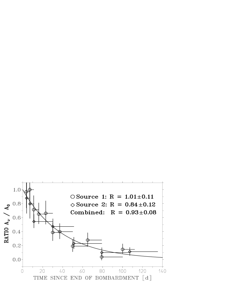
Figure 1: Individual run results of the GALLEX chromium neutrino source experiments, normalized to the known source activity, as a function of time after the end of neutron irradiation of the source. The horizontal bars indicate the durations of the exposures, the exponential curve the expectation from the decay of the source. Source I and Source II runs are represented by circles and diamonds, respectively.

An analysis of Source I and Source II yields $R=1.01\,\,^{+0.11}_{-0.10}$ and $R=0.84\,\,^{+0.12}_{-0.11}$, respectively, where $R$ is the source activity as deduced from the neutrino measurement normalized to the known true source activity. The combined analysis of both series results in $R=0.93\pm 0.08$, clearly demonstrating the absence of large systematic errors which could account for the observed 40% solar neutrino deficit.

A similar experiment has also been performed by the Sage collaboration. They got a quantitative recovery of $R=0.95\pm 0.12$ [6].

The fact that both experiments, though employing different chemistry, demonstrated in these experiments full efficiency, proves the trustworthiness of the radiochemical method and shows that the 40% solar neutrino deficit observed in the radiochemical gallium experiments cannot be ascribed to unknown systematic errors. In particular, the $\rm{{}^{51}Cr}$ neutrino energies nicely accommodating those from the solar $\rm{{}^{7}Be}$-branch, the full efficiency of the gallium experiments to $\rm{{}^{7}Be}$-neutrinos is demonstrated.

⁷¹As experiments

However, though the $\rm{{}^{51}Cr}$ source in Gallex did outperform the sun by more than a factor $15$ after insertion into the target tank, the experiments still are low statistics, involving only several dozens of neutrino produced $\rm{{}^{71}Ge}$ atoms. Therefore, at the very end of Gallex the collaboration has performed a large-scale test of potential effects of hot chemistry, which might lead to a different chemical behaviour of $\rm{{}^{71}Ge}$ produced in a nuclear reaction compared to the stable Ge carrier isotope: The in-situ production of $\rm{{}^{71}Ge}$ by $\beta-$decay of $\rm{{}^{71}As}$. A known quantity of $\rm{{}^{71}As}$ (O($10^{5}$) atoms) has been added to the tank (t-sample), where it decayed with $T_{1/2}=2.9\,$d to $\rm{{}^{71}Ge}$. Four runs have been made under different operating conditions (mixing, carrier addition, standing time), cf. table 2. For every spike a reference sample (e-sample) was kept aside, making possible to calculate the ratio of t- and e-sample which does not suffer from most of the systematic uncertainties associated with $\rm{{}^{71}Ge}$-counting.

Table 2: Experimental conditions and results (ratio t-sample/e-sample) of the $\rm{{}^{71}As}$ runs.

run	mixing conditions	Ge-carrier	standing	result
	$\rm[h\times m^{3}/h]$	addition	time	(tank / external)
A1	$\rm 22\times 5.5$	with As	$19.9\,$d	$1.01\pm 0.03$
	$\rm+0.17\times 60$
A2	$\rm 6\times 5.5$	no Ge-carrier	$19.9\,$d	$1.00\pm 0.03$
B3-1	$\rm 24\times 5.5$	after As	$2.0\,$d	$1.01\pm 0.03$
B3-2	—	after As	$22.0\,$d	$1.00\pm 0.03$

In all cases a quantitative recovery of 100% was achieved. This demonstrates on a 3%-level the absence of withholding effects even under unfavourable conditions like carrier-free operation.

Gallium Neutrino Observatory

With the $\rm{{}^{71}As}$-tests Gallex has completed its large-scale experimental program. However, solar neutrino measurements with a gallium target at Gran Sasso will be re-commenced in spring 1998 in the frame of the Gallium Neutrino Observatory (GNO) [2] which is designed for long-term operation covering at least one solar cycle. In its first phase GNO will use the $30\,$ton target of Gallex. However, for a second phase it is planned to increase the target mass to $60\,$tons and later to $100\,$tons. In addition, as it is equally important to decrease the systematic uncertainty, effort is made to improve $\rm{{}^{71}Ge}$ counting, both by improving the presently used proportional counters, and by investigating novel techniques like semiconductor devices and cryogenic detectors [1].

Acknowledgements

Our contribution to Gallex and Gno is supported by grants from the german BMBF, the SFB-375, and the Beschleunigerlaboratorium Garching.

Solar Neutrino Observation with Superkamiokande

Yoshiyuki Fukuda (for the Superkamiokande Collaboration)

Institute Cosmic Ray Research, University of Tokyo, Japan

Introduction

Superkamiokande, which is a second generation solar neutrino experiment, is an imaging water Cherenkov detector with 50,000 tons of pure water in the main tank. The detector is located 1000 m underground (2700 m water equivalent) in Kamioka Zinc mine in the Gifu prefecture of Japan, at 36.4^∘N, 137.3^∘E and 25.8^∘N geomagnetic latitude.

Figure 1: Schematic view of the Superkamiokande detector.

The detector consists of a main inner counter and an outer anti-counter. A schematic view of the detector is shown in Fig. 1. The inner counter is contained in a cylindrical stainless-steel tank and has a volume of 39.3 m in diameter $\times$ 42.0 m in height, containing 50,000 metric tons of water. A total 11,146 photo multipliers (PMTs) with 20 inch $\phi$ photo cathode area cover 40% of the entire inner surface of the tank. The fiducial mass for the solar neutrino measurement is 22,500 tons, with boundaries 2.0 m from the inner surface. On the other hand, a 4$\pi$ solid-angle anti-counter surrounding the inner counter is also a water Čerenkov counter of total mass 13,000 metric tons with 1850 PMTs to detect any signals coming from outside of the detector and to shield against gamma-rays and neutrons.

Calibrations

The timing calibration for all PMTs is done by the Xe lamp. We usually take those data for every 3 months and the maps of T-Q response for all PMTs are produced. This table is used for correct timing as a function of observed charge in real data analysis.

The variation of the water transparency is obtained by stopping muon spectrum (Michael spectrum). This is very important for obtaining the energy scale to be stable as a function of time. The energy is almost proportional to the number of hitted PMTs, however, the number maybe variable to the attenuation length of the water. Corrected number of hitted PMTs is very stable to the variation of water transparency. This is also confirmed by the $\gamma$-ray source which is emitted by the reaction of Ni(n,$\gamma$)Ni^∗. The absolute values of water transparency at various points of wavelength are measured by DYE-laser calibration. Recent water transparency itself is very stable.

The performances of the detector, such as the absolute energy scale, the energy resolution, the vertex resolution and the angular resolution are mainly calibrated by LINAC system. The LINAC can generate an electron beam with 5 MeV to 16 MeV. This beam is induced via beam pipe and bent by magnetic coil into the several positions of the tank. The typical values for each resolution is 16%, 70cm and 22 degree for 10 MeV electrons. The absolute energy for electron beam is calibrated by Ge solid state detector at each calibration time.

Monte Carlo simulation was tuned by the water transparency and other parameters to reproduce the energy scale in various tank positions within 1% difference between MC and real data.

Solar neutrino analysis

Superkamiokande has started from April 1996 and now processed about 400 days data for solar neutrinos measurement. Analysis procedures are (1) noise reduction, (2) vertex reconstruction and tight noise reduction, (3) spallation products cut, (4) fiducial volume (22.5 kton) cut and (5) gamma ray cut. Some of analysis techniques are similar to Kamiokande’s ones, however, most of them have been newly developed. In first step, we eliminate $\mu$ and decayed electron and several electronics noise. The second step reconstructs the vertex using the timing of hitted PMTs within selected 50 n second window. Main backgrounds in the residual data are spallation products. In order to eliminate those events, we used the likelihood method using the time difference and the distance between induced muon and those spallation events as a function of muon energy. We can reject most of spallation products with 20% dead time. In the last reduction, we reject external $\gamma$-rays coming from outside of the detector. Most of those events are sitting at very close to the edge of fiducial volume and have an opposite direction with respect to the detector wall. Event rate of the final sample is obtained by 175 events per day per 22.5 kton for 6.5 to 20 MeV.

Figure 2: (a) Angular distribution to the solar direction and (b) heliograph for 374.2 days data.

From 1st May 1996 to 22 Oct 1997, we obtained 374.2 days data from Superkamiokande measurement [1]. Figure 2 shows the angular distribution to the solar direction and the heliograph for obtained final sample. In Fig. 2(a), best fit line which is expected by MC is also shown. Extracted number of solar neutrinos is obtained by this fit as $4951^{+117.9}_{-111.3}$ for 374.2 days data. Observed ⁸B solar neutrino flux is given by

$$\phi(^{8}B)=2.37^{+0.06}_{-0.05}({\rm stat.})^{+0.09}_{-0.07}({\rm syst.})\times 10^{6}\,{\rm cm^{-2}sec^{-1}}$$

or by taking ratio to the BP95 flux [3];

$$\frac{\rm Data}{\rm SSM_{BP95}}=0.358^{+0.009}_{-0.008}({\rm stat.})^{+0.014}_{-0.010}({\rm syst.}).$$

Figure 3: (a) Energy spectrum, (b) Day/Night flux variation and (c) seasonal variation of obtained solar neutrino signal.

The systematic error related to the energy scale has been reduced by LINAC calibration and is obtained as 2.3%. Observed ⁸B neutrino flux is significantly deficit to the expectation of SSM(BP95) and it is consistent with the result from Kamiokande [2].

The energy spectrum of observed neutrinos is shown in Fig. 3(a). In this figure, expected spectra of MSW small angle parameter and just-so parameter are also shown. At first sight, small angle solution has better fit than flat (no oscillation) and just-so solution, but it is not significant within an experimental error. The day and night flux difference is obtained by;

$$\frac{D-N}{D+N}=-0.031\pm 0.024({\rm stat.})\pm 0.014({\rm syst.}).$$

If night data are divided into five bins, those differences are shown in Fig. 3(b). In this figure, typical day/night flux variation of the large angle and the small angle solutions are also shown. There is no significant difference in day/night fluxes in present observation. Also Fig. 3(c) shows the seasonal variation of solar neutrino fluxes. Each season is pile up among different years. Solid line corresponds to the expected variation from an eccentricity of the Sun orbit. Within experimental error, there is no seasonal variation in present analysis. Those results are also same ones from Kamiokande.

Two flavor neutrino oscillation

For astrophysical solution, it is generally difficult to explain the solar neutrino problem with the modification of SSM including the observations from helioseismology. On the other hands, the elementary particle solution using MSW neutrino oscillation [5] seems to be an excellent for explanation of the solar neutrino problem, because it can distort the spectra of solar neutrinos. Also MSW oscillation can give a effect in the day/night fluxes variation. As obtained by Fig. 3, our observed spectrum can be seen slightly as distorted one, but not seen in variance between day/night fluxes. Using these results, we can obtained the excluded region at 95% C.L. in MS diagram as shown in Fig. 4(a).

     

Figure 4: (a) 95% C.L. excluded region in MSW parameters. Inside of solid and dotted line are excluded by the observed energy spectrum and the day/night flux difference, respectively. (b) Allowed region in MSW parameters with measured ⁸B neutrino flux. Thick solid line, dashed line and thin solid line correspond to 95%, 90% and 68% C.L., respectively. Shaded region is allowed at 95% C.L. by Hata.

If we take the constraint of measured ⁸B solar neutrino flux, allowed region of 95%, 90% and 68% C.L. as shown in Fig. 4(b). From these figures, our results and the allowed region given by Ref. [4] are consistent in MSW oscillation analysis.

Summary

In summary, solar neutrino observation in Superkamiokande has started since May 1996 and has already taken 374.2 days data. The observed ⁸B solar neutrino flux is about 37% of the prediction from SSM(BP95) and it is almost consistent with the result from Kamiokande. Using LINAC calibration system, we can reduce the systematic errors related to the energy scale. Obtained energy spectrum is likely distorted and it is indicated that the new physical solution will be solved the solar neutrino problem. New challenge to lower threshold analysis ($\geq$ 5 MeV) has been started. Present radioactive (²²²Rn) level is about 3 mBq/m³, however, we will able to reduce that level to factor 1/5. Even though the present analysis, we have succeeded to extract solar neutrino signals from 5–6.5 MeV region. Those data will give a strong indication to the solution for the solar neutrino problem within a few years.

The Sudbury Neutrino Observatory

M.E. Moorhead (on behalf of the SNO Collaboration)

Particle and Nuclear Physics Laboratory, Keble Road, Oxford OX1 3RH, UK

The Sudbury Neutrino Observatory (SNO) [1] is a 1,000 ton heavy water (D₂O) Cherenkov detector in Sudbury, Ontario (Canada) which will start taking data in ‘98. The $\nu$ reactions which occur in D₂O and the extremely low background environment of the detector will allow the following measurements: i) the $\nu_{e}$ and $\nu_{x}$ (flavour independent) fluxes, and their ratio, for ⁸B solar $\nu$’s, ii) the energy spectrum of ⁸B $\nu_{e}$’s above 5 MeV, iii) time dependence in the ⁸B flux, and iv) detailed studies of the $\nu$ burst from a galactic supernova, including a search for $\nu_{\mu}$ and $\nu_{\tau}$ masses above 20 eV. For the ⁸B solar $\nu$ measurements, the $\nu_{e}/\nu_{x}$ flux ratio and the $\nu_{e}$ energy spectrum constitute two separate tests of $\nu$ oscillations which are both independent of solar model flux calculations [2]. If the currently favoured MSW solution [3] of the solar neutrino problem is correct then the $\nu_{e}/\nu_{x}$ flux ratio should provide conclusive proof of oscillations with one year’s data yielding a 17 sigma departure from unity (statistical error only).

The detector is situated two kilometers underground in a dedicated laboratory that has been excavated in the Creighton nickel mine of INCO Corporation. This laboratory comprises facilities for changing into clean-room clothing, a lunch room, a car wash for bringing equipment into the clean area, a utility room where the H₂O and D₂O systems are located, a control room and a $30~{}{\rm m}\times 23~{}{\rm m}$ barrel shaped cavity for the detector itself. The walls of the cavity have been coated with concrete and low-activity Urylon, a water proof radon barrier. Inside this cavity is located a 12 m diameter spherical acrylic vessel (AV), recently completed, for containing the D₂O neutrino target. Almost completely surrounding this AV, stands a 17 m geodesic sphere supporting 9,500 20-cm-Hamamatsu PMTs, each of which is equipped with a light reflecting concentrator to increase its effective photocathode area by a factor 1.7. Beginning in March ‘98, the detector will be filled with 7,000 tons of high purity H₂O outside the acrylic vessel (to act as shielding for high energy gamma rays coming from the rock and the PMTs) and 1,000 tons of D₂O inside the AV. The filling will take between 3–4 months and hence data taking will begin in mid-98.

The event rates for solar $\nu$’s, assuming the full SSM ⁸B flux [4], and for a supernova (SN) at the center of our galaxy are given in Table 1. Apart from the neutral current (NC) reaction, all of the events are detected by the array of 9,500 PMTs via the Cherenkov radiation emitted by a single electron (or positron) of energy $\geq 5$ MeV, the detector’s threshold. The NC reaction produces a free neutron in the D₂O which can be detected, after thermalization, by observing a subsequent neutron capture reaction. There are three capture reactions of interest depending on what additives are placed in the D₂O:

i) Pure D₂O: In the case of no additive there is a 30% probability of capture on deuterium, which produces a 6.25 MeV gamma. This gamma converts to electrons by Compton scattering and pair production, and the resulting Cherenkov light is detected by the PMTs. Five hundred events a year are expected above the detector’s 5 MeV threshold.

ii) MgCl₂: Dissolving 2 tons of MgCl₂ in the D₂O gives an 83% chance of neutron capture on ³⁵Cl which produces an 8.5 MeV gamma cascade. The higher efficiency and Q-value of this capture (c.f. capture on deuterium in the pure D₂O case) increases the number of detected events by a factor of 5 to 2,500 per year.

iii) ³He Counters: An array of ³He proportional counters [5] (5 cm diameter tubes of 800 m total length) placed vertically in the D₂O in a square grid of 1m spacing, gives a 42% chance of neutron capture on ³He. The energy and rise-time of the signals are used to separate $n$-capture (2,000 per year) from internal alpha and beta backgrounds.

The dominant background for all these NC detection methods will probably come from photodisintegration of deuterium which produces free neutrons that are indistinguishable from NC neutrons. Thus, the detector components have been carefully selected for extremely low levels of thorium and uranium chain contamination so that the photodisintegration rate is small compared with the NC rate. This small residual photodisintegration rate must be measured, in order to subtract its contribution to the neutron capture signal. Several methods have been developed for this purpose: i) radiochemical extraction and counting of ²²⁸Th, ²²⁶Ra, ²²⁴Ra, ²²²Rn and ²¹²Pb, ii) analysis of low energy signals seen by the PMT array, iii) delayed coincidences between signals seen by the PMT array, and iv) prompt and delayed coincidences between signals seen by the PMTs and signals in the ³He proportional counters.

Table 1: Neutrino event rates in SNO (including detection efficiency). SSM refers to the event rate per year for ⁸B solar neutrinos assuming the standard solar model [4] and the small angle MSW solution [3]. SN refers to a type II supernova at a distance of 10 kpc (the center of the galaxy).

Neutrino reaction		SSM	SN
Charged Current (CC):	$\nu_{e}+d\rightarrow p+p+e^{-}$	3000	80
Neutral Current (NC):	$\nu_{x}+d\rightarrow p+n+\nu_{x}$	2500	300
Electron Scattering (ES):	$\nu_{e,x}+e^{-}\rightarrow\nu_{e,x}+e^{-}$	400	20
Anti-neutrino CC in D2O:	$\bar{\nu}_{e}+d\rightarrow n+n+e^{+}$	0	70
Anti-neutrino CC in H2O:	$\bar{\nu}_{e}+p\rightarrow n+e^{+}$	0	350

BOREXINO

L. Oberauer (for the Borexino Collaboration)

Technische Universität München, Physik Department E15, 85747 Garching, Germany
and Sonderforschungsbereich 375 Teilchen-Astrophysik

Physics Goals and Neutrino Detection with Borexino

The aim of the solar neutrino experiment Borexino is to measure in real time the solar neutrino flux with low energy threshold at high statistics, and energy resolving via pure leptonic neutrino electron scattering $\nu+e\to\nu+e$.

Motivation for Borexino comes from the long standing solar neutrino puzzle. Data analysis of the existing experiments leads to the assumption of severe suppression of the solar ${}^{7}{\rm Be}$-branch, which probably cannot be explained by modifications of the standard astrophysical model of the sun. The monoenergetic ${}^{7}{\rm Be}$-neutrinos give rise to a compton like recoil spectrum in Borexino. Its edge will be at 660 keV, significantly higher than the aimed energy threshold of ca. 250 keV. Thus ${}^{7}{\rm Be}$-neutrino detection is very efficient in Borexino.

Assuming validity of the standard model a counting rate for ${}^{7}{\rm Be}$-neutrinos, which would consist in this case purely as $\nu_{e}$, of roughly 55/day in Borexino is expected.

In scenarios of total neutrino flavour conversion (i.e. for neutrino mass differences $\Delta m^{2}\approx 10^{-6}{-}10^{-5}\,\,{\rm eV}^{2}$) a reduced flux of approximately 12/day would be measured due to the lower cross section of $\nu_{\mu,\tau}$ scattering, which occurs only via neutral current interaction.

In case of vacuum oscillations (i.e. for neutrino mass differences $\Delta m^{2}\approx 10^{-10}\,\,{\rm eV}^{2}$) Borexino would see a distinct time dependent periodical neutrino signal due to the seasonal eccentricity of the earth’s orbit around the sun.

For neutrino mass differences in the range of $\Delta m^{2}\approx 10^{-7}\,\,{\rm eV}^{2}$ and for large mixing Borexino should see a ‘day/night’ effect due to electron neutrino regeneration during the path through the earth.

Borexino also can serve for additional projects in neutrino physics. Search for a magnetic moment can be performed by means of terrestrial neutrino sources by investigating the electron recoil shape at low momentum transfer. Via the inverse beta-decay $\bar{\nu}_{e}+p\to e^{+}+n$ Borexino can look for signals from geophysical neutrinos as well as for neutrinos emitted by european nuclear power plants. The latter would serve as a long baseline neutrino oscillation experiment probing the so-called large mixing angle solution for the solar neutrino problem.

The Detector and Background Considerations

The detector is shielded successively from outer radioactivity by means of an onion-like structure. Here the adjacent inner layer serves as shielding and has to provide an increased purity in terms of internal radioactivity.

Borexino is placed in hall C of the underground laboratory at Gran Sasso, Italy. An overburden of ca. 3500 m.w.e. suppresses the cosmic muon flux to roughly $1/{\rm m}^{2}$. The outer part of the detector consists of a steel tank with 18 m in height and diameter. Inside this ‘external’ tank a stainless steel sphere will support 2200 phototubes on the inside and 200 tubes at the outside. Most of the tubes inside the sphere will be equipped with light guides in order to increase the geometrical coverage and hence the energy resolution. Between external tank and sphere high purity water will serve as shielding against external gamma rays and as active Cherenkov counter against cosmic muons. The steel sphere will be filled with a tranparent, high purity buffer liquid which itself holds a nylon sphere, filled with organic scintillator. The active scintillator mass will be around 300 t. By means of time of flight measurements event position can be reconstructed and a fiducial volume for solar neutrino interaction defined. The latter should be about 100 t, establishing a counting rate of 55 neutrinos per day according to the standard solar model. The outer part of the scintillator sphere serves as active shielding.

The demands on purity in terms of radioactivity in Borexino, especially for the scintillator itself, are very severe. In order to be able to extract a clear signal from background events also in case of total flavour conversion, an intrinsic concentration in Uranium and Thorium of ca. $10^{-16}$ should not be exceeded significantly. The amount of ${}^{14}{\rm C}/^{12}{\rm C}$ must not be higher than $\approx 10^{-18}$. In order to test scintillating materials a large Counting Test Facility (CTF) has been built up in hall C of the underground laboratory at Gran Sasso, which resembles to a small prototyp (ca. 5 t of scintillator) of Borexino. From beginning of 1995 until summer 1997 several tests about the feasibilty of Borexino including procedures to maintain the purity of the scintillator has been performed, which showed very encouraging results: ${}^{14}{\rm C}/{}^{12}{\rm C}=1.85\cdot 10^{-18}$, ${}^{238}{\rm U}=(3.5\pm 1.3)\cdot 10^{-16}\,\,{\rm g/g}$, ${}^{232}{\rm Th}=(4.4\pm 1.5)\cdot 10^{-16}\,\,{\rm g/g}$. A complete discussion of the CTF results including experimental techniques for further background suppression is given in [1] and [2]. Details about the experimental setup of the CTF can be found in [3].

Highly developed neutron activation analysis of scintillation samples performed in Munich is now sensitive in the same regime. For uranium an upper limit of ${}^{238}{\rm U}<2\cdot 10^{-16}\,\,{\rm g/g}$ (90% CL) has been obtained. In addition concentration values or limits have been measured by this method for a various amount of isotopes, including man-made nuclei. For details, see [4].

Background studies for Borexino include also the interaction of cosmic muons. The direct detector response on muons has been determined by a coincidence measurement between the CTF and a muon telescope on top of it. The time distribution of such events can be used to discriminate between muon events and neutrino candidates at a level of 98%. However, to reach the sensitivity needed to reach the goals in Borexino, the leak rate for muons must not exceed a level of $\approx 10^{-4}$. Our design of the muon veto system therefore is threefold: The outer region between external tank and steel sphere acts as Cherenkov counter, a special configuration of the tubes inside the sphere will act as an additional muon identification system, and finally the offline study of event topology like the time structure will help to suppress this kind of background sufficiently.

Cosmogenic generation of radioactive nuclei has been sudied this fall at the 180 GeV muon beam at SPS in CERN. Most dangerous source of events will come from ${}^{11}{\rm C}$-production in the scintillator and surrounding buffer liquid. However, the energy spectrum of these events is between 1 MeV and 2 MeV since the decay mode is positron decay at 1 MeV endpoint energy. Thus the detection of ${}^{7}{\rm Be}$-neutrinos is not affected, however that of pep-neutrinos.

Prospects

Borexino is an international collaboration of about 60 scientists. Approved funding already comes from INFN (Italy) and from BMBF and DFG (Germany). A substantial part should also be covered by NSF (USA) in the near future. Work on the external tank of Borexino is almost completed. We expect to finish with the inner steel sphere in 1999. Simultaneously the CTF will be upgraded. Finally it will serve as test facility for Borexino scintillator procurement in batch mode. Given full funding also for our american collaborators first data taking may be expected at the end of the year 2000.

Measurements of Low Energy Nuclear Cross Sections

M. Junker (for the LUNA Collaboration)

Laboratori Nazionali Gran Sasso, Assergi (AQ), Italy
and Institut für Experimentalphysik III, Ruhr-Universität Bochum, Germany

The nuclear reactions of the pp-chain play a key role in the understanding of energy production, nucleosynthesis and neutrino emission of the elements in stars and especially in our sun [1]. A comparison of the observed solar neutrino fluxes measured by the experiments GALLEX/SAGE, HOMESTAKE and KAMIOKANDE provides to date no unique picture of the microscopic processes in the sun [2]. A solution of this so called “solar neutrino puzzle” can possibly be found in the areas of neutrino physics, solar physics (models) or nuclear physics. In view of the important conclusions on non-standard physics, which might be derived from the results of the present and future solar neutrino experiments, it is essential to determine the neutrino source power of the sun more reliably.

Due to the Coulomb Barrier involved in the nuclear fusion reactions, the cross section of a nuclear reaction drops nearly exponentially at energies which are lower than the Coulomb Barrier, leading to a low-energy limit of the feasible cross section measurements in a laboratory at the earth surface. Since this energy limit is far above the thermal energy region of the sun, the high energy data have to be extrapolated down to the energy region of interest transforming the exponentially dropping cross section $\sigma(E)$ to the astrophysical $S$-factor $S(E)=\sigma(E)\,E\,{\exp(2\,\pi\,\eta)}$, with the Sommerfeld parameter given by $2\,\pi\,\eta=31.29\,Z_{1}\,Z_{2}(\mu/E)^{1/2}$ [1]. The quantities $Z_{1}$ and $Z_{2}$ are the nuclear charges of the interacting particles in the entrance channel, $\mu$ is the reduced mass (in units of amu), and $E$ is the center-of-mass energy (in units of keV). In case of a non resonant reaction $S(E)$ may then be parameterized by the polynomial $S(E)=S(0)+S^{\prime}(0)E+0.5\,S^{\prime\prime}(0)E^{2}.$

As usual in physics, extrapolation of data into the “unknown” can lead onto “icy ground”. Although experimental techniques have improved over the years to extend cross section measurements to lower energies, it has not yet been possible to perform measurements within the thermal energy region in stars.

For nuclear reactions studied in the laboratory, the target nuclei and the projectiles are usually in the form of neutral atoms/molecules and ions, respectively. The electron clouds surrounding the interacting nuclides act as a screening potential: the projectile effectively sees a reduced Coulomb barrier. This leads to a higher cross section, $\sigma_{\rm s}(E)$, than would be the case for bare nuclei, $\sigma_{\rm b}(E)$, with an exponential enhancement factor $f_{\rm lab}(E)=\sigma_{\rm s}(E)/\sigma_{\rm b}(E)\simeq\exp(\pi\eta\,U_{\rm e}/E)$ [3, 4] where $U_{\rm e}$ is the electron-screening potential energy (e.g. $U_{\rm e}\simeq Z_{1}\cdot Z_{2}\cdot e^{2}/R_{\rm a}$ approximately, with $R_{\rm a}$ an atomic radius). For a stellar plasma the value of $\sigma_{\rm b}(E)$ must be known because the screening in the plasma can be quite different from that in laboratory studies [5], and $\sigma_{\rm b}(E)$ must be explicitly included in each situation. Thus, a good understanding of electron-screening effects is needed to arrive at reliable $\sigma_{\rm b}(E)$ data at low energies. Low-energy studies of several fusion reactions involving light nuclides showed [6, 7, 8] indeed the exponential enhancement of the cross section at low energies. The observed enhancement (i.e. the value of $U_{\rm e}$) was in all cases close to or higher than the adiabatic limit derived from atomic-physics models. An exception are the ³He+³He data of Krauss et al. [10], which show apparently no electron screening down to $E$=25 keV, although the effects of electron screening should have enhanced the data at 25 keV by about a factor 1.2 for the adiabatic limit $U_{\rm e}$=240 eV. Thus, improved low-energy data are particularly desirable for this reaction.

The low-energy studies of thermonuclear reactions in a laboratory at the earth’s surface are hampered predominantly by the effects of cosmic rays in the detectors. Passive shielding around the detectors provides a reduction of gammas and neutrons from the environment, but it produces at the same time an increase of gammas and neutrons due to the cosmic-ray interactions in the shielding itself. A 4$\pi$ active shielding can only partially reduce the problem of cosmic-ray activation. The best solution is to install an accelerator facility [11] in a laboratory deep underground [9]. The worldwide first underground accelerator facility has been installed at the Laboratori Nazionali del Gran Sasso (LNGS) in Italy, based on a 50 kV accelerator. This pilot project is called LUNA and has been supported since 1992 by INFN, BMBF, DAAD-VIGONI and NSF/NATO.

The major aim of the LUNA project is to measure the cross section of ³He(³He,2p)⁴He which is one of the major sources of uncertainties for the calculation of the neutrino source power. It has been studied previously [10] down to about $E_{\rm cm}$=25 keV, but there remains the possibility of a narrow resonance at lower energies that could enhance the rate of path I at the expense of the alternative paths of the pp-chain that produce the high-energies neutrinos ($E_{\rm\nu}>0.8$ MeV). The LUNA–facility allows to study this important reaction over the full range of the solar Gamow Peak, where the cross section is as low as 8 pbarn at $E_{\rm cm}$=25 keV and about 20 fbarn at $E_{\rm cm}$=17 keV.

Figure 1 shows the results obtained in the energy region between $E_{\rm cm}$=25 keV and $E_{\rm cm}$=20.7 keV. The lowest counting rate was of 3 events per day at $E_{\rm cm}$=20.7 keV. At this energy about 1000 Cb of ³He⁺ have been accumulated on the target. The data obtained at higher energies (450 kV accelerator in Bochum) with the LUNA setup [11] are included for completeness. Previous data obtained [10] at $E_{\rm cm}$=25 are also shown in figure 1. The LUNA data have been obtained at energies within the solar Gamow Peak, i.e. below the 21 keV center of this peak, and represent the first measurement of an important fusion cross section in the thermal energy region.

Figure 1: The $S(E)$ factor of ³He³He from [10] and the present work. The dashed and solid curves represent $S_{\rm b}(E)$ and $S_{\rm s}(E)$ respectively. The solar Gamow Peak is shown in arbitrary units.

The astrophysical $S$-factor has been extrapolated to zero energy [12]:

$$S(0)=5.40\pm 0.05{\rm(stat)}\pm 0.30{\rm(sys)}\pm 0.30{\rm(screen)}.$$

The first error contains the statistical error (one standard deviation) including counting statistics and apparative variations of pressure, beam power and temperature measurement. The second error is the systematical error (one standard deviation) including uncertainties in pressure, beam energy and power, efficiency and energy loss data. The 10% error of the energy loss data transforms to an uncertainty of 0.1 to 0.2 keV in the effective energy. This in turn leads to an error of 1 to 3.5 % for the astrophysical $S$-factor. This is due to the exponential decrease of the cross section at low energies [12]. The third component of the error results from the lack of understanding of electron screening: Fitting all existing data sets with $S(0)$, $S^{\prime}(0)$, $S^{\prime\prime}(0)$ and $U_{\rm e}$ as free parameter gives an Electron Screening Potential $U_{\rm e}$ of 323 eV with $S(0)=5.30$ MeVb. Fixing $S(0)$, $S^{\prime}(0)$ and $S^{\prime\prime}(0)$ at energies higher than 100 keV (where the electron screening effect is neglectible) gives $S(0)=5.1$ MeVb. In turn fitting $U_{\rm e}$ in a second step including also the low energy data gives $U_{\rm e}=432$ eV. A fit to the data assuming no electron screening gives $S(0)=5.7$ MeVb. The adiabatic limit for $U_{\rm e}$ based on theoretical atomic physics is 240 eV. The first two methods give $U_{\rm e}$ values higher than the adiabatic limit (240 eV), consistent with observations in other fusion reactions. The difference between observed and predicted $U_{\rm e}$ values is not understood at present giving a considerable uncertainty on $S(0)$.

Based on the success of the LUNA project and on the fruitful international collaboration (in particular the support provided by LNGS), further experiments with the 50 kV machine for a better understanding of the electron screening effect are planned. The proposed reactions are D(p,$\gamma$)³He, D(³He,p)⁴He, ⁷Li(p,$\alpha$)⁴He and ¹¹B(p,$\alpha$)⁷Be($\alpha$)$\alpha$. In addition, some interesting aspects in nucleosynthesis of the early universe are related to the low energy cross section of the first reaction [13].

While studying these reactions an enlarged LUNA II collaboration will install a 200 kV accelerator facility at Gran Sasso to study the pp–reactions ³He($\alpha$,$\gamma$)⁷Be and ⁷Be(p,$\gamma$)⁸B and the key reaction of the CNO–cycles, ¹⁴N(p,$\gamma$)¹⁵O, at energies far below the present limits. All these reactions are critical to the solar neutrino puzzle. The reaction rate of ¹⁴N(p,$\gamma$)¹⁵O is also one of the ingredients needed to determine the theoretical scenario used to constrain both the age and the distance of the oldest stellar system in our galaxy, namely the Globular Clusters. In such a way, more stringent limits to the cosmology will be obtained.

In addition, the new 200 kV accelerator will afford the study of many (p,$\gamma$) reactions of the NeNa and MgAl cycles below an incident proton energy $E_{\rm p}$=200 keV. Experimental data about these channels, very important for the understanding of nucleosynthesis processes, are up today still missing or very uncertain. For example the NeNa cycle may play a role in understanding the almost pure ²²Ne abundance found in meteorites samples, while the MgAl cycle may provide the mechanisms for production of ²⁶Al, the decay of which gives rise to the ²⁶Mg/²⁷Al anomaly found in some meteorites. All the involved (p,$\gamma$) cross sections of these cycles are scarcely known at low energies: a continuation of the underground experimental program of the LUNA experiment could be devoted in the future to the measurement of these channels for proton incident energies below 200 keV, where many unmeasured resonances are present [14]. For example the strength of the low lying resonances in the reaction ²⁵Mg(p,$\gamma$)²⁶Al, which is crucial for the production of ²⁶Al, could be experimentally determined for the first time. Also the other reactions of these cycles can be investigated using stable targets and accelerator and detector systems of the LUNA experiment.

Solar Neutrinos: Where We Are and What Is Next?

G. Fiorentini

Dipartimento di Fisica dell’Universitá di Ferrara and Istituto Nazionale di Fisica Nucleare, Sezione di Ferrara, I-44100 Ferrara, Italy

What has been Measured?

All five experiments report a deficit of solar neutrinos with respect to the predictions of Standard Solar Models (SSMs), see Ref. [1].

What Have We Learnt on Solar Neutrinos, Independently of SSMs?

Actually, the solar neutrino puzzle (SNP) is not just the discrepancy between experimental results and the predictions of standard solar models. Rather, experimental results look inconsistent among each other with the only assumption that the present total neutrino flux can be deduced from the present solar luminosity, unless something happens to neutrinos during the trip from Sun to Earth, see Fig. 1 and Refs. [1, 2, 3].

What Has Been Calculated?

Accurate predictions of solar neutrino fluxes are anyhow extremely important. If neutrino masses (differences) are as small as suggested by several proposed solutions to the SNP, then the only way to measure neutrino masses is through the interpretation of future solar neutrino experiments, which requires accurate theoretical predictions of solar properties.

Refined solar models are thus necessary. All these have to be confronted with the powerful helioseismic constraints, see Ref. [4], particularly for a quantitative (and conservative) determination of the accuracy of solar properties as deduced from helioseismology.

Recent SSM calculations, using accurate equations of state, recent opacity calculations and including microscopic diffusion, look in agreement with heliosesimology, see Figs. 3 and 3 and Ref. [4]. Alternative solar models should be as successful as these are [5, 6].

Actually, one can exploit helioseismology within a different strategy. One can relax some assumptions on the most controversial ingredients of solar models (e.g. opacity and metal abundance) and determine them by requiring that helioseismic constraints are satisifed. These helioseismically constrained solar models (HCSM) all yield the same central temperature within about one percent [7]. The main uncertainties for the determination of solar neutrino fluxes arise now from nuclear physics measurements. After the succesful LUNA experiments at LNGS [8], the main uncertainties are now from the ³He+⁴He and ⁷Be+p reactions.

What Is Missing?

In a prophetical paper of 1946 [9] Bruno Pontecorvo wrote: “direct proof of the existence of the neutrino $\ldots$ must be based on experiments the interpretation of which does not require the law of conservation of energy, i.e. on experiments in which some characteristic process produced by free neutrinos $\ldots$ is observed.”

The situation now looks very similar, just change existence with nonstandard properties, in that the strongest argument for a particle physics solution to the SNP arises from energy conservation (the luminosity constraint) and actually we need a direct footprint of some neutrino property, not predicted within the minimal standard model of electroweak interactions.

The four most popular particle physics solutions (small and large angle MSW effect, just so oscillations and universal oscillations) all predict specific signatures which are being or will be tested by the new generation of experiments (Superkamiokande, Borexino, SNO, $\ldots$), see Table 1.

The hypothesis of universal oscillation proposed in Ref. [10] has just been falsified by the recent negative result of CHOOZ [11]. This nice and small (in comparison with the gigantic solar neutrino devices) experiment at a nuclear reactor is cleaning some of the fog in the air.

Let us wait and wish that (at least) one of the fingerprints of neutrino oscillations is detected by the new experiments.

Table 1: The proposed solutions, their fingerprints and the experiments looking at them.

Proposed solutions Signatures Oscillation spectral Day-night Seasonal CC/NC at reactor deformation variation modulation events MSW small angle NO TINY TINY NO YES MSW large angle NO TINY YES NO YES JUST-SO NO YES NO YES YES Universal oscil. YES NO NO NO YES Experiment CHOOZ SUPERKAM. SUPERKAM. BOREXINO SNO Data now now now 2000 2000

Figure 1: The ⁸B and ⁷Be+CNO neutrino fluxes, consistent with the luminosity constraint and experimental results for standard neutrinos. The dashed (solid) lines correspond to the central ($\pm 1\sigma$) experimental values for chlorine [13], gallium [14] and $\nu$-$e$ scattering experiments [15]. The dashed area corresponds to the region within $2\sigma$ from each experimental result. The predictions of solar models including element diffusion (full circles) [12, 16, 17, 18] and neglecting diffusion (open circles) [19] are also shown. The dotted lines indicate the behaviour of nonstandard solar models with low central temperature [1].

Figure 2: The difference between $U$ as predicted by selected solar models, $U_{\rm mod}$, and the helioseismic determination, $U_{\odot}$, normalized to this latter (thin line). The allowed area is that within the thick lines. BP95 is the model with metal and He diffusion of Ref. [12]; JCD96 is the“model S” of Ref. [20]; D96 is the “model 0” of Ref. [21]; CDR97 is the “best” model with He and heavier elements diffusion of Ref. [17].

Figure 3: Helioseismic determinations and solar model predictions of properties of the convective envelope. The box defines the region allowed by helioseismology. Open circles denote models without diffusion, squares models with He diffusion, full circles models with He and heavier elements diffusion [4].

Phenomenology of Supernova Explosions

Wolfgang Hillebrandt

Max-Planck-Institut für Astrophysik, D-85748 Garching, Germany

Abstract

An attempt is made to match observed properties of supernovae, such as spectra, lightcurves etc. with theoretical ideas and predictions. It is demonstrated that neither do observational data constrain the models in a unique way nor does theory allow for an unambiguous interpretation of the data. Possible improvements on the theoretical side are briefly discussed.

Some Observational Facts

In general, supernovae are classified according to their maximum light spectra. Those showing Balmer lines of H are called Type II’s, and all the others are of Type I. Those Type I’s which show a strong Si absorption feature at maximum light are named Type Ia, and the others are Ib’s or Ic’s, depending on whether or not they have also He I features in their spectra [1]. At later times, several months after the explosion, when the supernova ejecta become optically thin, Type II spectra are dominated by emission lines of H, O, and Ca, whereas Type Ia’s have no O, but Fe and Co. Type Ib,c’s, on the other hand side, show emission lines of O and Ca, just like the Type II’s [1]. However, the spectral classification is not always as clear. For example, SN 1987K started out as a Type II with H lines, but changed into a Type Ib,c like spectrum after 6 months [2].

As far as the light curves are concerned, Type II’s seem to be more complicated than Type I’s. Type II-L are characterized by a peak lasting for about 100 days, followed by a “linear” decay in the blue magnitude vs. time diagram. In contrast, Type II-P’s have a somewhat wider peak, followed by a “plateau” phase and an occasionally rather complicated tail decaying not like a single exponential. Typically, Type II-L’s are brighter than Type II-P’s in the blue. In addition, there are objects like SN 1987A which possess a very complicated light curve, with an early narrow peak, a first minimum, followed by a broad hump after a few months, and a final nearly exponential decay with indications of some flattening at late times. SN 1987A-like objects are much dimmer than all other Type II’s [1].

In contrast, all Type Ia light curves are quite similar, making them good candidates for standard candles to measure the cosmic distance scale. Moreover, since they are the brightest among all supernovae, they can be observed even at high redshifts and, in fact, a Type Ia supernova at a redshift of about 1 has recently been observed [3]. Although their absolute peak luminosity may vary by about one magnitude, an observed correlation between the luminosity and light curve shape (the brighter ones have broader light curves) allows one to correct for the differences. So recently observations of Type Ia’s have become a powerful tool in attempts to determine cosmological parameters [3]. Of course, one has to make sure that the supernovae one is observing are indeed of Type Ia, and not of Type Ib,c which are intrinsically fainter, but this can be achieved if a spectrum near maximum light is available.

Other observational information on supernovae is, in general, less solid. With the exception of SN 1987A, we do not have direct information on the properties of the progenitors, the energetics, or the masses of the ejecta and of the (compact) remnants, if there are any. Indirect information can be obtained from the light curves and the spectra leading, however, to an “inverse” problem as far as theoretical interpretations are concerned.

Theoretical Classification

The theoretical classification of supernovae is usually done according to the suspected progenitor stars and the explosion mechanism, and it dates back to a classic paper of Fred Hoyle and Willy Fowler in 1960 [4]. Based on very few observational facts available at that time, they postulated that Type II supernovae are the consequence of an implosion of non-degenerate stars, whereas Type I’s are the result of the ignition of nuclear fuel in degenerate stars, and today this is still believed to be true in general, if “Type I’s” are substituted by “Type Ia’s”.

Figure 1: Theoretical classification scheme of supernovae according to their progenitors.

Figure 2: Theoretical classification scheme of supernovae according to their energy sources.

To be more specific, the present theoretical classification schemes based on progenitor properties and the energetics of the explosion are given in Figs. 1 and 2, respectively. It is now generally believed that Type II and Ib.c supernovae stem from collapsing massive stars with and without hydrogen envelopes, respectively, and that SN Ia originate from explosions of white dwarfs, although the way to explosion (accretion vs. merging of two white dwarfs) as well as the mass of the white dwarf (Chandrasekhar vs. sub-Chandrasekhar mass) just prior to the explosion are still heavily disputed (see Ref. [5] and references therein).

The classification with respect to the energetics is even more complex, and a variety of possible models is available with no unique and well accepted answer. For example, in the case of thermonuclear explosions, it is not even clear what the mode of propagation of the burning front is, and observations supply poor constraints only. A (fast) deflagration wave in a Chandrasekhar-mass white dwarf can explain the spectra and light curves of Type Ia’s, but so can deflagrations changing into detonations at low densities with or without pulsations (so-called delayed detonations), or even pure detonations in stars with low enough densities are not completely ruled out. As far as the physics of core collapse supernovae is concerned, the situation is not significantly better. Whether or not rotation is important, whether or not magnetic fields play any role, whether neutrinos are diffusively or convectively transported from the cooling proto-neutron star to the stellar mantle, and many other questions are largely unanswered.

Merging Theory and Observations

Of course, a simple way to try to improve the rather unsatisfactory situation outlined in the previous section is to call for more observations. Since computing realistic theoretical light curves and synthetic spectra for a given supernova model has become feasible recently (although computing reliable spectra for Type Ia’s still requires novel techniques) high quality data might help to rule out certain possibilities. But as long as most theoretical models contain a large number of more or less free parameters one may doubt the success of this approach.

A few examples may serve as illustrations. As long as for a thermonuclear explosion the propagation velocity of the burning front and the degree of mixing can still be treated as free functions, it is easy to fit a given light curve and spectrum of a Type Ia supernova (see, e.g. Ref. [1]), but one does not prove that the model is correct. Similarly, in the core collapse scenario, neutrinos can transfer momentum to the mantle of a star and cause a supernova explosion, provided their luminosity is sufficiently high. If this luminosity results from low opacities or from convection does not matter. Also, only thousands of neutrino events from a single supernova seen in a neutrino detector could possibly tell the difference. Finally, a similar momentum transfer can, in principle, be mediated by appropriate combinations of rotation and magnetic fields. Again, a lucky accident of a galactic supernova may supply enough data, including detections of gravity waves, to eliminate several models, but only for one special event and not for the entire class.

Therefore, it appears to be more promising to search for ways to reduce the freedom one still has in building theoretical models. An obvious possibility is to replace parameter studies by first principle calculations, whenever this is possible. Again, a few examples are given to demonstrate that there is plenty of room for improvements. A first and obvious example is again neutrino transport in core collapse supernovae. One will note that very primitive (and likely incorrect) approximations for neutrino interactions with dense nuclear matter are commonly used in all hydrodynamic simulations, and only very recently first attempts have been made to compute those cross sections on the basis of microscopic theories [6, 7]. Similarly, well-developed methods to calculate the properties of dense nuclear matter are available, but the equations of state used in numerical studies are still computed ignoring nucleon-nucleon correlations, despite the fact that the stiffness of the equation of state is very important ingredient. As far as thermonuclear models are concerned, numerical methods to handle turbulent combustion are presently developed for combustion in engines and for reactor safety, and there is no principle problem in applying them also to supernovae. Moreover, simple microscopic models can be calibrated to laboratory combustion experiments, which again will help to reduce the number of parameters.

In conclusion, not underrating the importance of new and better observational data in supernova research, I still think that most of the progress in the near future has to come and can come from theory.

Supernova Rates

Bruno Leibundgut

European Southern Observatory
Karl-Schwarzschild-Strasse 2, D-85748 Garching, Germany

Apart from stellar winds supernovae are the only mechanism which releases chemically processed material from stars into the interstellar and intergalactic gas. They are almost exclusively responsible for the chemical enrichment of galaxies and the universe as a whole. As one of the end stages of stellar evolution and one of the production channels of pulsars and black holes supernovae are also placed at a major link of stellar and non-stellar matter. They further inject kinetic energy into the interstellar gas which may be important for gas heating, cosmic rays, and possibly the kinematics of galaxies.

Knowing the frequency of supernovae means to know the rate with which these processes occur. Having further knowledge of the temporal evolution of this frequency can provide the chemical history of galaxies. Supernova statistics are thus a main ingredient in the study of formation and transformation of matter in the universe.

Recent reviews of supernova rates has been published by van den Bergh & Tammann (1991), Tammann (1994), and Strom (1994). The visual searches have been summarized by van den Bergh and McClure (1994). A series of papers by Cappellaro et al. (1993a, b, 1997) have explored the derivation of the supernova rate in detail. SN statistics starting from the available SN catalogs and exploiting various indirect routes were presented by Tammann, Löffler, & Schröder (1994).

Supernova statistics make use of minimal information about the explosions themselves. The main ingredients are the type of the explosion and a crude description of the parent population in which the explosion occurred. This is normally restricted to the morphological type of the host galaxy. The last piece of information is the time when the explosion took place. The frequency of supernovae $\nu_{\rm SN}$ is described as the ratio of known SNe $N_{\rm SN}$ over the total galaxy luminosity $L_{\rm gal}$ per unit time $t$

$$\nu_{\rm SN}=\frac{N_{\rm SN}}{L_{\rm gal}\cdot t}.$$

The SN rate is normally expressed in Supernova Units (SNu) which corresponds to one supernova per $10^{10}$ (blue) solar luminosities per 100 years.

Although in principle easy to determine, the derivation of supernova rates suffers from a number of problems. Supernovae are very rare objects. The number of supernovae in galaxies with known parameters (morphological type, luminosity, color) is rather small. There are about 60 to 80 supernovae per year, but only about 10 bright supernovae in nearby galaxies (cf. Timmes & Woosley 1997). The surveyed galaxy sample has to be well described and defined. Many supernovae occur in galaxies which are not part of the current catalogs, thus being lost for the derivation of the rates. Another problem is the control times, i.e. the time the galaxies have actually been surveyed for supernovae. Large corrections can be incurred when the galaxies are not observed frequently.

The small number statistics becomes even more apparent when we consider that the known supernovae have to be split into a number of subsamples to become meaningful. Typically there is a subdivision into three SN types and about five galaxy morphologies, which immediately creates 15 bins to group the supernovae. With typical numbers of about 200 SNe (e.g. van den Bergh & McClure 1994, Cappellaro et al. 1997) in the sample the rates are not immune against small number statistics.

Over 1200 supernovae been discovered to date. Many of these objects are not classified and can not be used for the statistics. However, about 80% of all supernovae since 1989 have a type associated. The distribution is roughly 55% SNe Ia (thermonuclear explosions of white dwarfs) and 41% SNe II and SNe Ib/c (core-collapse in massive stars). Since SNe Ia are on average about 2 magnitudes brighter than other supernovae, they can be detected over a larger volume and thus are present at a higher percentage. Excluding all the supernovae from searches specifically targeted at very distant supernovae (Perlmutter et al. 1997, Leibundgut & Spyromilio 1997), which mostly are Type Ia, we arrive at a near equipartition between thermonuclear and core-collapse SNe (48% SNe Ia and 49.5% SNe II and SNe Ib/c since 1989). With the same argument as above (SNe Ia more luminous) we can immediately conclude that core-collapse SNe are more frequent than thermonuclear SNe in the nearby universe. This result is further amplified by dust obscuration which affects core-collapse SNe stronger than thermonuclear SNe.

Several corrections enter the determination of supernova rates. The best known is the Shawn effect (Shawn 1979) which describes the effect of supernovae lost in the glare of centers of galaxies. Visual and CCD searches are less affected than older photographic searches which lose the contrast in bright regions. Absorption can obscure supernovae in the discs of galaxies and if, as currently believed, core-collapse supernovae stem from massive stars and are thus more affected by dust, the derived SN statistics are skewed. Several proposals how to correct for dust have been put forward (e.g. van den Bergh & Tammann 1991). The luminosity of the various subtypes of supernovae differs by factors of about 10 and the differences in light curve shapes introduces varying control times for the SN classes. These have to be factored in when the SN rate is derived.

There are two distinct approaches to derive SN statistics. The ‘search technique’ uses only supernovae which have been discovered in controlled searches. The most recent and complete description of this method is given by Cappellaro et al. (1997). The advantage here is that the control times and the galaxy sample are defined very well. The drawback is the small number of supernovae in the sample. Cappellaro et al. (1997) had to discard about half of the discovered supernovae, because they appeared in galaxies which are not part of the catalogs. They were left with 110 supernovae from five searches which have lasted for almost 20 years and amounted to a total of 42500 years $\times 10^{10}L_{\odot}$ control time (sometimes referred to as ‘galaxy years’).

The ‘catalog technique’ makes use of all supernovae discovered in a known galaxy sample (Tammann et al. 1994). This maximizes the number of supernovae as all supernovae discovered in galaxies of the sample are included in the statistics, but strong assumptions on the control time have to be made. The latter quantity can be derived very badly as serendipitous SN discoveries enter the catalogs.

Despite all these problems, there is a fair agreement for the rates of thermonuclear supernovae (Type Ia) in star-forming (spiral) galaxies. The distribution is independent of the detailed morphological type of the galaxy at about 0.2 SNu. A large discrepancy exists for old stellar systems (elliptical galaxies) for which Tammann et al. find a rate increasing to a level three times higher, while Cappellaro et al.  actually find indication of slightly lower SN Ia rate in ellipticals. There is only a very small number of supernovae known in elliptical galaxies, however, and the statistics are very uncertain.

Core-collapse supernovae (Types II and Ib/c) have not been observed in elliptical galaxies. Their rate increases with the fraction of young stars in galaxies, i.e. the morphological type. The most prolific supernova producers are Sc and Sd galaxies with about 1.2 SNu. There is a discrepancy of about a factor of two in the absolute rates between Tammann et al. and Cappellaro et al. for all galaxy types. The relative rates, however, agree quite well. The SN rates in irregular galaxies are largely undetermined due to the small numbers of known SNe.

The Galactic SN rate is about $20\pm 8$ per millennium. This number depends on the morphological type and the total blue luminosity of the Galaxy. There are 6 historical supernovae on record (van den Bergh & Tammann 1991) which implies that roughly 2/3 of all Galactic supernovae have been hidden. Supernovae in the Local Group have been observed in M31 (S And: SN 1885A) and in the Large Magellanic Cloud (SN 1987A). The prediction for the Local Group is slightly above 2 (excluding the Galaxy), which appears consistent. The small observational baseline, however, excludes any firm conclusion from such a comparison.

Pulsar Velocities and Their Implications

A.G. Lyne

University of Manchester, Jodrell Bank, Macclesfield, Cheshire SK11 9DL, UK

In several respects, the Galactic distribution of pulsars mimics the distribution of population I species, such as young stars, HII regions and supernova remnants. In particular, the galactocentric radial distributions are very similar. However, the widths of the distributions in distance from the Galactic plane, Z, differ by nearly a factor of 10. Gunn and Ostriker (1970) [1] realised that this difference could result from high velocities which may be given to pulsars at birth, possibly arising in the violence of their formation in supernova collapse. It was several years later before the first measurement of the proper motion of a pulsar gave direct evidence for this hypothesis [2]. Transverse velocities are now known for more than 100 pulsars and their high values are generally well established.

In this review, I describe briefly the techniques used in the measurement of pulsar velocities, summarise the main features of the distribution of the velocities and discuss their implications for the physics of the formation events and for their spatial distribution.

There are two main techniques which have been used for the determination of pulsar velocities, in both cases providing the transverse components of the velocity only. These techniques respectively involve the measurement of proper motion and of the velocity of the interstellar scintillation pattern across the Earth. Proper motions are determined from high-resolution radio interferometry or from timing measurements. Like optical techniques, the former involves measurement of the position of a pulsar relative to a nearby source over a period of time. With modern instruments, position accuracy of 10 milliarcseconds (mas) is readily achievable, so that only a few years are required to give proper motion errors of only a few mas/yr [3, 4, 5, 6, 7]. Timing measurements can give similar precision in principle, but are usually limited by irregularities in the rotation rate of the pulsar, known as “timing noise,” which is predominant in young pulsars. However, timing is particularly useful for millisecond pulsars which have very stable rotation and whose narrow pulses allow very high accuracy.

Estimates of pulsar transverse velocities $V_{t}$ are then obtained from the proper motion $\mu$ (mas/yr) and the distance $D$ (kpc): $V_{t}=4.74\,\mu D$ km/s. The distance $D$ is obtained from the dispersion measure and an electron density model [8] which is based upon a number of independent distance measurements. Nearly 100 such measurements of transverse velocity are available.

Figure 1: The motions of pulsars relative to the galactic plane. Pulsars are represented as filled circles in galactic longitude and Z-distance, the tail representing its approximate motion in the past 1 Myr.

The velocities of pulsars estimated from observations of the speed of the interstellar scintillation patterns [9, 10] are considered rather less reliable than the more direct proper motion measurements, mainly because it has recently been shown [11] that the values are systematically low by an average factor of 2 because of a localisation of the scattering medium close to the galactic plane. There are about 71 pulsars for which scintillation speeds are available [10], although most of these pulsars have rather better proper motion measurements, leaving 27 which have only scintillation measurements. Combining both techniques gives a sample of about 100 values of $V_{t}$, of which about 8 are upper limits.

From this sample, the mean transverse velocity is found to be $\langle V_{t}\rangle=300\pm 30$ km/s. With a small number of exceptions, the velocity vectors shown in Fig. 1 demonstrate a clear movement away from the galactic plane, consistent with pulsars being formed from massive, young, population I stars close to the plane and receiving velocities of a few hundred km/s at the same time. How large are the typical space velocities? Unfortunately, there is a selection effect visible in the data in which high velocity pulsars quickly move away from the plane of the Galaxy and become undetectable, leaving an excess of low-velocity pulsars. This effect can be minimised by considering the velocity distribution of only the youngest pulsars, which cannot have moved far since birth. The 29 pulsars with characteristic age of less than 3 Myr give $\langle V_{t}\rangle=350\pm 70$ km/s. Monte Carlo simulations show that the mean space velocity required to give such an observed transverse velocity distribution is $\langle V_{s}\rangle=450\pm 100$ km/s [12].

There are two other pieces of evidence which support such high velocities: the increase of the mean distance of pulsars from the plane as a function of characteristic age and the movement of a small number of pulsars from the centres of the putative supernova remnants associated with their birth [12].

Similar analyses for the 13 millisecond pulsars with proper motion measurements give $\langle V_{t}\rangle=88\pm 19$ km/s and $\langle V_{s}\rangle=130\pm 30$ km/s, showing them also to be a rather high-velocity population. Not surprisingly, no migration from the galactic plane is seen, because of their large ages. These velocities probably represent the low-velocity end of the “kick” spectrum—higher velocity kicks are likely to disrupt any binary system, preventing any millisecond pulsar formation by accretion spin-up in a binary system.

Clearly, the high velocities explain why only a few percent of pulsars are in binary systems, compared with the high proportion of the likely progenitor stars in binaries. However, the high velocities pose something of a problem for the retention of pulsars in globular clusters: the velocities mostly exceed the cluster escape velocities and yet there is a substantial pulsar population which has remained gravitationally bound [13, 14]. It is also worth noting that about half of the pulsar population will escape the gravitational potential well of the Galaxy, ending up in intergalactic space, the remainder being in a large galactic halo.

There has been much speculation on the origin of the high velocities, the three main possibilities being the disruption of binary systems, an electrodynamic “rocket” effect in the early life of the pulsars and asymmetry in the supernova explosions. The first two have great difficulty in explaining the size of the velocities and the most likely origin seems to lie in the supernova explosion itself. The high momentum asymmetry of the neutron star after the explosion must be matched by that of either the ejecta or neutrinos. The origin of the asymmetry is not clear, although both convection and the magnetic field have been cited as the possible determining agents. It is worth noting that up to now, the magnetic properties of the neutron stars do not seem to implicate the magnetic field in the production of the high velocities.

Convection in Newly Born Neutron Stars

W. Keil

Max-Planck-Institut für Astrophysik
Karl-Schwarzschild-Str. 1, D-85740 Garching, Germany

Introduction

Observations of SN 1987A instigated recent work on multi-dimensional numerical modeling of Type-II supernova explosions. Two-dimensional (2D) simulations [1, 2, 3, 4] indicate that overturn instabilities and mixing in the $\nu$-heated region between PNS and supernova shock may indeed help $\nu$-driven explosions to develop for conditions which do not allow explosions in spherical symmetry. Nevertheless, a critical investigation of the sensitivity of the explosion to the value of the $\nu$ flux from the neutron star [3, 4] cannot confirm claims that a “convective engine” ensures the robustness of the explosion for a wide range of conditions. Instead, the explosion turns out to be extremely sensitive to the $\nu$ fluxes from the inner core. Explosions can occur in 2D as well as in 1D, provided the $\nu$ luminosity is large enough. Similarly, for too small core $\nu$ fluxes, strong convective overturn in the $\nu$-heated region cannot develop and the explosion fizzles. These findings are supported by recent simulations of Mezzacappa and collaborators [5]. In addition, all currently successful numerical models of supernova explosions produce nucleosynthesis yields that are in clear contradiction with observational abundance constraints. These facts indicate severe problems of the numerical modeling of the explosion. The first 2D simulations of the evolution of the nascent neutron star [6] suggest that long-lasting quasi-Ledoux convection in the PNS can significantly raise the $\nu$ luminosities and may have a positive impact on the supernova explosion and conditions for explosive nucleosynthesis.

Results of Two-Dimensional Hydrodynamical Simulations

Our simulations were performed with an elaborate description of the nuclear equation of state [7] and the $\nu$ transport and were started with a PNS model of Bruenn [8] at $\sim 25$ ms after core bounce. These calculations showed that driven by negative lepton fraction and entropy gradients convective activity can encompass the whole PNS within $\sim 1\,{\rm s}$ and can continue for at least as long as the deleptonization of the PNS takes place. Because of the importance of the diffusive $\nu$ transport this convection is not an ideal, adiabatic Ledoux convection. Also specific thermodynamical properties of the nuclear equation of state have to be taken into account. In differentially rotating PNSs stabilizing angular momentum distributions seem to suppress convection near the rotation axis.

Figure 1: Panel a shows the absolute values of the convective velocity for a non-rotating PNS model $0.7~{}{\rm s}$ after the start of the simulation in units of $10^{8}\,{\rm cm/s}$. The computation was performed in an angular wedge of $180^{\circ}$ assuming axisymmetry. Panel b displays the relative deviations of the lepton fraction $Y_{\rm lep}$ from the angular means $\langle Y_{\rm lep}\rangle$ at each radius for $t=0.7~{}{\rm s}$. The maximum deviations are of the order of 50%. Lepton-rich matter rises while deleptonized material sinks in.

The convective pattern is extremely non-stationary and has most activity on large scales with radial coherence lengths of several km up to $\sim 10\,{\rm km}$ and convective “cells” of 20^∘–30^∘ angular diameter, at some times even 45^∘ (Fig. 1a). The maximum convective velocities are $\sim 5\times 10^{8}\,{\rm cm/s}$, but peak values of $\sim 10^{9}\,{\rm cm/s}$ can be reached. Relative deviations of the lepton fraction $Y_{\rm lep}$ from the angular mean can be several 10% in rising or sinking buoyant elements (Fig. 1b), and for the entropy ($S$) they can reach 5% or more. Rising flows always have larger $Y_{\rm lep}$ and $S$ than their surroundings.

Figure 2: Panel a shows the recoil velocity of our PNS model in km/s as a function of time resulting from stochastical asymmetries in the $\nu$ flux. Panel b displays the spectral energy density of the emitted gravitational radiation caused by mass motions and anisotropic $\nu$ emission.

Since convective activity continues for more than 1 s in a large region of the PNS, convective $\nu$ transport shortens the cooling and deleptonization timescales of the PNS compared to results of 1D simulations and enhances the calculated $\nu$ luminosities of the star by up to 65%. The latter can have important influence on the interpretation of the measured $\nu$ signal from SN 1987A and might change limits of various quantities in nuclear and elementary particle physics which have been derived from these measurements. Moreover, the enhancement of the $\nu$ fluxes can also have important consequences for the explosion mechanism of the supernova, because it aids $\nu$-driven explosions. The faster deleptonization modifies the luminosity ratio of $\nu_{e}$ and $\bar{\nu}_{e}$ in such a way that the electron fraction $Y_{e}^{\rm ej}$ in the $\nu$-heated SN ejecta will be raised during the first few 100 ms after core bounce, but it will be lowered for $t\mathrel{\vbox{\offinterlineskip\hbox{$>$}\hbox{$\sim$}}}1$ s compared to 1D simulations. This might help to solve the severe problems of the nucleosynthesis in current models of Type-II supernovae which disregard long-lasting convective activities in the PNS. Finally, convection in the PNS causes stochastical asymmetries of the $\nu$ flux. In our calculation the resulting recoil accelerates the PNS to $\sim$ 9 km/s during 1.2 s (Fig. 2a). This is too small to explain measured proper motions of pulsars of a few 100 km/s. Both convective mass motions and anisotropic $\nu$ emission are a source of gravitational waves for more than 1 second (Fig. 2b). Most of the gravitational radiation is emitted at frequencies of 300–1400 Hz.

Acknowledgements

We thank S.W. Bruenn for kindly providing us with the post-collapse model used as initial model in our simulations. Support by the “SFB 375-95 für Astro-Teilchenphysik” of the German Science Foundation is acknowledged.

Anisotropic Supernovae, Magnetic Fields,
and Neutron Star Kicks

H.-Th. Janka

Max-Planck-Institut für Astrophysik
Karl-Schwarzschild-Str. 1, D-85740 Garching, Germany

Abstract

Hydrodynamic instabilities during the supernova explosion and neutrino cooling phase lead to stochastic acceleration of the nascent neutron star and are hardly able to account for recoil velocities $\,\hbox{\hbox{$>$}\kern-8.00003pt\lower 4.30554pt\hbox{$\sim$}}\,100\,$km/s. It is argued that an internal magnetic field of $\sim 10^{14}\,{\rm G}$ can define a preferred direction of the neutrino emission with an anisotropy of several per cent which is sufficiently large to produce kicks even in excess of 1000 km/s and thus can explain the fastest motions of observed pulsars.

Introduction

Pulsars are observed with large mean velocities of several 100 km/s (see A. Lyne, this conference, for references to observations), and a few neutron stars are measured with velocities of more than 1000 km/s. Similar velocities can also be deduced from associations of neutron stars with nearby supernova remnants. Binary evolution arguments strongly suggest that neutron stars experience a recoil already during their birth in the supernova explosion of a massive progenitor star (e.g., [1, 2]). The reason for this acceleration is not finally understood and several mechanisms were proposed or investigated, among them anisotropic core collapse and mass ejection during the supernova explosion (e.g., [3]), large-scale hydrodynamic instabilities during the explosion (e.g., [4, 5]), or anisotropic neutrino emission of the cooling proto-neutron star [6], for example associated with convective processes (e.g., [4, 5, 7]), magnetic fields (e.g., [8, 9]), or neutrino oscillations (e.g., [10, 11]). A 1% anisotropy of the neutrino emission during the neutrino cooling phase of the newly formed neutron star would be sufficient to accelerate the remnant to about 300 km/s.

While some of the proposed kick mechanisms are highly speculative and involve one or even more components of new or non-standard physics (e.g., neutrino masses or magnetic moments, superstrong magnetic fields), other mechanisms are unsatisfactory in the sense that they rely on certain initial conditions in the collapsing stellar core or in the nascent neutron star which are very specific and cannot be easily justified from stellar evolution calculations (e.g., special magnetic field configurations or density distributions to produce global anisotropies). More “natural” anisotropies which develop in self-consistent simulations from hydrodynamic instabilities without the use of specially chosen initial conditions, on the other hand, turned out to be sufficient to account for small velocities of a few 10 km/s but seem hardly able to explain the very fast motions of pulsars.

Hydrodynamic Instabilities and Neutron Star Convection

For example, anisotropic mass motions due to convection in nascent neutron stars lead to gravitational wave production and anisotropic emission of neutrinos (see W. Keil, this conference). The angular variations of the neutrino flux determined by 2D simulations are of the order of 5–10% [12, 13]. With the typical size (10–30 degrees angular diameter) and short coherence times (a few milliseconds) of the convective structures, however, the global anisotropy of the neutrino emission from the cooling proto-neutron star is certainly less than 1% (more likely only 0.1%) and observed high kick velocities in excess of 300 km/s can definitely not be explained. In the simulation described by Keil, the determined recoil velocity is disappointingly low, only about 10 km/s! There is no reason to expect this case to be an especially unfavorable one. Even worse, in three dimensions the convective elements tend to become smaller than in 2D because of fragmentation and turbulent energy transport from larger to smaller scales which is forbidden in 2D due to angular momentum conservation. This makes large recoil velocities of neutron stars by the described mechanism even more unlikely.

Convective motions in the neutron star have important consequences for the magnetic field structure. Specific kinetic energies of the order of ${1\over 2}v^{2}\sim 10^{17}\,$erg/g could lead to equipartition fields of more than $B\sim 10^{16}\rho_{14}^{1/2}\,$G. Such strong fields increase the neutrino opacities [9, 14] and could affect the anisotropy of the neutrino emission. In the dense medium of the neutron star, where the electrons are degenerate, the influence of the magnetic field on the charged-current reactions becomes essential when the characteristic energy of an electron on a Landau level reaches the size of the electron chemical potential, i.e. when $B\,\hbox{\hbox{$>$}\kern-8.00003pt\lower 4.30554pt\hbox{$\sim$}}\,B_{\rm c}\cdot(\mu_{e}/m_{e}c^{2})\sim 5\times 10^{15}\ldots 2\times 10^{16}\,$G where $B_{\rm c}=m_{e}^{2}c^{3}/(\hbar e)=4.4\cdot 10^{13}\,{\rm G}$. The presence of such strong fields changes the phase space distribution of the electrons and thus the cross section for $\nu_{e}$ absorption on neutrons [14]. Whether this results in sizable neutron star kicks or not will depend on the strength and structure of the magnetic fields inside the neutron star. Turbulent convective motions will certainly produce a much more irregular magnetic field distribution than the idealized mirror asymmetry assumed by Bisnovatyi-Kogan [9] who suggested that an initial, strong toroidal field component is amplified by a wound-up poloidal field in one hemisphere, whereas both toroidal field components (the initial one and the one produced by winding the poloidal field) are superposed destructively in the other hemisphere. A more irregular field evolution will imply a much smaller global anisotropy of the neutrino emission than estimated in reference [9].

Rapid rotation of the collapsed stellar core has very important effects on the development and strength of convection. Two-dimensional, self-consistent hydrodynamic simulations [12, 13] reveal that a positive gradient of the specific angular momentum in the nascent neutron star stabilizes hydrodynamically unstable entropy or lepton number stratifications. This positive gradient of the specific angular momentum suppresses convective motions near the rotation axis and allows strong convection to occur only close to the equatorial plane. Therefore, the neutrino emission is convectively enhanced around the equatorial plane while it is essentially unchanged near the poles. For the same reason, the magnetic field structure may retain an initial dipole component and irregular fields must be expected to be produced by convective mass motions only in a belt around the equator.

Parity Violation and Cumulative Asymmetry

According to a recent suggestion by Horowitz and Li [15], a global anisotropy of the neutrino emission of the nascent neutron star could originate from the cumulative effect of a large number of neutrino scatterings off polarized nucleons in the magnetized stellar medium. Although the polarization corrections to a single neutrino-lepton interaction are small, typically of the order of only $10^{-5}$ of the cross section [15, 16], Horowitz and Li recognized that a macroscopic asymmetry can build up because the anisotropy of the neutrino flux increases with the average number of scatterings per neutrino, i.e. with the optical depth of the medium. The polarization term in the cross section represents a slightly different chance for a neutrino to be scattered into the direction of the external magnetic field than into the opposite direction, or means a tiny enhancement of the scattering probability of neutrinos moving into (or opposite to) the field direction. Formally, the neutrino flux is not only described by a diffusive propagation mode (proportional to the gradient of the neutrino energy density), but an additional “advective” vector component in the magnetic field direction (see [17, 18]). The ratio between advective and diffusive component grows approximately linearly with the scattering optical depth $\tau$. Physically, this can be understood [15] by recalling that a diffusing particle has travelled a mean distance $d=\sqrt{N}\lambda$ after $N$ steps with (constant) scattering mean free path $\lambda$. If the particle has a tiny chance $P$ to be scattered into the field direction, the distance it has propagated along the field after $N$ scatterings is $l=PN\lambda$. Therefore the relative anisotropy increases as $l/d\propto P\sqrt{N}\propto\tau$ (for $P\sqrt{N}\ll 1$). The second proportionality holds because the optical depth is defined as $\tau=d/\lambda$, thus $\tau=\sqrt{N}$.

The discussed process would be highly interesting if the magnetic fields required to create a few per cent anisotropy of the neutrino emission of a neutron star were much smaller than the very strong fields ( $>$$\sim$  several $10^{15}\,{\rm G}$) where the neutrino opacity is affected by the change of the electron phase space distribution. Horowitz and Li [15] have only considered very simple situations of scattering media to show the fundamental characteristics of the cumulative process and have disregarded essential complications of neutrino transport in neutron stars, e.g., neutrino absorption, transport of different neutrino types with opposite signs of the polarization terms, and the feedback of the transport on the energy distribution in the neutron star. The question must be asked whether the proposed cumulative process leads to a global anisotropy of the neutrino emission of the nascent neutron star and how large this anisotropy can be for a given magnetic field.

Figure 1: Neutrino luminosity and emission anisotropy as functions of time step for two Monte Carlo simulations of the neutrino cooling of a one-dimensional toy model of a neutron star. $L=L_{+}+L_{-}$ is the total neutrino luminosity, $\Delta L=L_{+}-L_{-}$ $\Delta L=L_{+}-L_{-}$ the luminosity difference between the two hemispheres (both normalized to the maximum luminosity $L_{\rm max}$), $E=E_{+}+E_{-}$ the energy radiated in neutrinos, and $\Delta E=E_{+}-E_{-}$ the energy difference (both normalized to the final energy $E_{\rm max}$). The integral asymmetry of the neutrino emission is given by the parameter $q=\Delta E/E$ which approaches nearly 16% towards the end of the simulations. The three-dimensional asymmetry in the integrated neutrino luminosity, $q_{\rm 3D}$, would be smaller by a factor 1/2 (for small anisotropies) compared to the displayed one-dimensional results. The Monte Carlo simulations were performed for models with total optical depths of $\tau=30$ (left) and $\tau=100$ (right), where the opacity polarizations were rescaled such that the results should be identical if the anisotropy grows linearly with the optical depth. The very good agreement between both calculations (left and right) thus confirms the scaling of the cumulative anisotropy with the optical depth of the star.

The neutron star situation was more realistically investigated by Lai and Qian [18] who estimated a maximum recoil velocity of about 200 km/s for average magnetic fields of $\sim 10^{14}\,{\rm G}$, provided the magnetic field in a nascent neutron star possesses a strong dipole component. Their analysis, however, is based on the assumption that neutrinos and antineutrinos, in particular $\nu_{e}$ and $\bar{\nu}_{e}$, have the same opacity for interactions with the stellar medium. Therefore their kicks are only produced by the deleptonization neutrinos which carry away only a minor fraction ($\sim$ 10%) of the gravitational binding energy of the neutron star which is released by neutrino emission. This assumption, however, leads to a large underestimation of the recoil acceleration [19].

Monte Carlo simulations [19] which include neutrino production and absorption, different opacities and polarizations for different neutrino and antineutrino flavors ($\nu_{e}$, $\bar{\nu}_{e}$, and heavy lepton neutrinos $\nu_{x}$ and $\bar{\nu}_{x}$), and the evolution of the stellar background in a simplified but reasonable, approximative description, suggest that a polarization term in the neutrino-nucleon scattering opacity of $\kappa_{\rm s,pol}/\kappa_{\rm s}\sim 10^{-5}$ can lead to a global asymmetry $q$ of the integrated neutrino luminosity of about 16% for the one-dimensional (plane) case (Fig. 1). Taking into account projection effects by multiplying this result with 1/2, the corresponding three-dimensional asymmetry $q_{\rm 3D}$ is estimated to about 8%, i.e. $q_{\rm 3D}\sim 0.08\cdot\left[\left(\kappa_{\rm s,pol}/\kappa_{\rm s}\right)/10^{-5}\right]$. This can be related to the anisotropy parameter $\alpha_{\rm 3D}$ for the momentum transfer to the neutron star: $\alpha_{\rm 3D}={\textstyle{2\over 3}}q_{\rm 3D}\sim 0.05\cdot\left[\left(\kappa_{\rm s,pol}/\kappa_{\rm s}\right)/10^{-5}\right]$. The effective polarization of neutrino-nucleon scatterings depends on the magnetic field strength $B$, the plasma temperature $T$, and the abundances $Y_{n}$ and $Y_{p}$ of neutrons and protons, respectively:

$${\kappa_{\rm s,pol}\over\kappa_{\rm s}}\,\sim\,\left(6.4\times 10^{-5}-13.3\times 10^{-5}{Y_{p}\over Y_{n}}\right)\cdot\left(1+1.134\,{Y_{p}\over Y_{n}}\right)^{\!-1}\cdot{B_{14}\over T_{10}}\;,$$ (1)

where $B_{14}$ is measured in $10^{14}\,{\rm G}$ and $T_{10}$ in $10\,{\rm MeV}$. Using representative values for temperature and composition during the phase when most of the gravitational binding energy of the neutron star is radiated away in neutrinos, $T=10\,...\,30\,{\rm MeV}$, $Y_{n}=0.8\,...\,0.9$, and $Y_{p}=1-Y_{n}=0.2\,...\,0.1$, a space-time average of $\kappa_{\rm s,pol}/\kappa_{\rm s}\sim 10^{-5}$ can be expected for a mean interior magnetic field $\langle B_{z}\rangle$ of the neutron star of $\sim 10^{14}\,{\rm G}$. This leads to an estimated recoil velocity of

$$v_{\rm ns} \cong 1800\left({\alpha_{\rm 3D}\over 0.05}\right)\left({1.4\,M_{\odot}\over M_{\rm ns}}\right)\left({E_{\nu}\over 3\times 10^{53}\,{\rm erg}}\right)\,{\rm km\,s^{-1}}$$ (2)

$$\sim 1800\left({\langle B_{z}\rangle\over 10^{14}\,{\rm G}}\right)\left({1.4\,M_{\odot}\over M_{\rm ns}}\right)\left({E_{\nu}\over 3\times 10^{53}\,{\rm erg}}\right)\,{\rm km\,s^{-1}}\;.$$

The reason for a nearly 10 times larger anisotropy compared to the result found by Lai and Qian [18] is twofold. During deleptonization and neutronization the neutron star plasma becomes increasingly asymmetric, i.e. the abundance of protons decreases and the plasma becomes neutron-rich. On the one hand, the unequal concentrations of neutrons and protons cause different opacities for $\nu_{e}$ and $\bar{\nu}_{e}$, on the other hand the growing abundance of neutrons implies an increase of the total polarization of the nucleonic medium because the contributions from neutrons and protons have opposite signs and partly cancel. For a typical post-collapse composition, $Y_{p}\approx 0.35$ and $Y_{n}\approx 0.65$, this cancellation is severe and reduces the polarization to roughly 1/8 of the value for a neutronized medium with $Y_{p}\approx 0.1$ and $Y_{n}\approx 0.9$. The latter composition is representative of the late Kelvin-Helmholtz cooling phase after the deleptonization of the proto-neutron star. Most (60–90%) of the neutrino energy is radiated during this phase which is therefore decisive for a “rocket engine” effect by asymmetric neutrino emission.

Of course, the estimated velocity in Eq. (2) is an upper limit which could be realized only if the interior magnetic field were uniform in the $z$-direction throughout the neutron star. Convective processes that reach deep into the star will certainly destroy the ordered structure of the field. In case of rapid rotation of the newly formed neutron star (rotation periods of a few milliseconds), however, convection can develop only near the equatorial plane but is suppressed near the rotation axis where an ordered field structure could persist in a large fraction of the neutron star volume.

Conclusions

If parity violation of weak interactions plays the crucial role to kick pulsars and if convection is important during the early phases of a neutron star’s life, one would therefore conclude that the observed velocities of fast pulsars between several $100\,$km/s and more than $1000\,$km/s require interior magnetic fields from a few $10^{13}\,{\rm G}$ to $\sim 10^{14}\,{\rm G}$, and that the largest velocities might indicate rapid rotation of the newly formed neutron star.

Acknowledgements

This work was supported by the “Sonderforschungsbereich 375-95 für Astro-Teilchenphysik” der Deutschen Forschungsgemeinschaft. Stimulating discussions with S. Hardy, G. Raffelt, and S. Yamada are acknowledged.

Spectrum of the Supernova Relic Neutrino
Background and Evolution of Galaxies

Katsuhiko Sato$\,{}^{1,2}$, Tomonori Totani$\,{}^{1}$ and Yuzuru Yoshii$\,{}^{2,3}$

${}^{1}\,$Department of Physics, School of Science, the University of Tokyo
7-3-1 Hongo, Bunkyo-ku, Tokyo 113, Japan
 
${}^{2}\,$Research Center for the Early Universe, School of Science, the University of Tokyo
7-3-1 Hongo, Bunkyo-ku, Tokyo 113, Japan
 
${}^{3}\,$Institute of Astronomy, Faculty of Science, the University of Tokyo
2-21-1 Osawa, Mitaka, Tokyo 181, Japan

Abstract

Neutrinos emitted from the supernovae which have ever occurred in the universe should make a diffuse neutrino background at present. This supernova relic neutrino background (SRN) is one of the targets of the Superkamiokande (SK) detector which will be constructed in this year and the SRN, if at all detected, would provide a new tool to probe the history of supernova explosions in the universe. The SRN spectrum is calculated by using a realistic, time-dependent supernova rate derived from a standard model of galaxy evolution based on the population synthesis method. The expected event rate at the SK is also calculated. The SRN spectrum we show here is the most realistic at present, because the largest uncertainty in previous theoretical predictions has come from unrealistic assumptions of the supernova rate so far made. Our major results include: (1) the supernova rate is much higher in the early phase of evolution of galaxies and there appears a hump in the SRN spectrum in the low-energy region of $\mathrel{\mathop{\hbox{\lower 2.15277pt\hbox{$\sim$}\kern-8.00003pt\lower-3.01385pt\hbox{$<$}}}}5$ MeV, (2) the SRN flux depends on the Hubble constant ($H_{0}$) in a way approximately proportional to $H_{0}^{2}$ and only weakly on the density parameter of the universe ($\Omega_{0}$) and a cosmological constant ($\lambda_{0}$), (3) the uncertainty in the star formation history of spiral galaxies affects the resulting SRN flux by about a factor of 3, and (4) the plausible event rate at the SK is 1.2 yr^-1 in the observable energy range of $15$–$40$ MeV. Such a low event rate is due mainly to a quite low supernova rate at present which is averaged over the morphological types of galaxies. The most optimistic rate in our model is found to be 4.7 yr^-1 in the same energy range, and if more events are detected, we will have to reconsider our current understanding of collapse-driven supernovae and evolution of galaxies.

Summary and Conclusions

We have calculated the SRN spectrum and also the expected event rate at the SK detector by using a realistic, time-dependent supernova rate from a reasonable model of galaxy evolution based on the population synthesis method. This model of galaxy evolution has been used to investigate the geometry of the universe from comparison with the number counts of faint galaxies, and the predicted number counts are well consistent with the recent observations. In our analysis the absolute SRN flux in the model is determined from the luminosity function and the mass-to-luminosity ratio of nearby galaxies, but not from the present supernova rate of our Galaxy which is subject to a large margin of uncertainty.

In the model we used, the supernova rate is much higher in the early phase of elliptical galaxies, and more than half of total supernovae explode during the initial 1 Gyr from the formation of galaxies. Thereafter, the supernova rate in spiral galaxies becomes dominant and the total number of supernovae until present is consistent with the nucleosynthesis requirement. A constant rate of supernova explosions, which was assumed in most of previous papers, is not justified from a viewpoint of galaxy evolution, and therefore the SRN spectrum we show here is the most realistic at the present time.

Supernovae produced at a very high rate in the early phase of ellipticals are responsible for the appearance of a hump in the low-energy part ($\mathrel{\mathop{\hbox{\lower 2.15277pt\hbox{$\sim$}\kern-8.00003pt\lower-3.01385pt\hbox{$<$}}}}$ 5 MeV) of the SRN spectrum, because the energy of neutrinos from those supernovae is degraded by the cosmological redshift effect. This energy degradation makes early neutrinos unobservable and the high supernova rate causes almost no enhancement in the event rate in the observable energy range of 15–40 MeV at the SK.

We used a low-density, flat universe with a non-zero $\Lambda$ as a standard cosmological model ($\Omega_{0}$=0.2, $\lambda_{0}=0.2$, and $h=0.8$), and investigated the SRN spectrum for other cosmological models relative to the standard model. The SRN flux strongly depends on $H_{0}$ as roughly proportional to $H_{0}^{2}$. The SRN flux changes with $\Omega_{0}$ and $\Lambda$ in a way that smaller $\Omega_{0}$ and/or larger $\Lambda$ suppresses the flux in the high-energy region ($\mathrel{\mathop{\hbox{\lower 2.15277pt\hbox{$\sim$}\kern-8.00003pt\lower-3.01385pt\hbox{$>$}}}}$ 10MeV), however, these changes are rather small. The shape of the SRN spectrum is almost insensitive to either of the above three parameters.

We investigated the uncertainty of the SRN spectrum from the model of galaxy evolution. The simple, one-zone and $n=1$ (S1) model, which we use as a standard evolution model of spiral galaxies, gives an intermediate SRN flux among the four different models of spiral galaxies considered in this paper (for explanation of the models see Refs. [1, 2]). The difference between the highest flux from the I1 model and the lowest flux from the S2 model is within a factor of 3. In the case of elliptical galaxies, however, the different SFRs hardly change the SRN spectrum in either shape or intensity. The effect of changing $z_{F}$ on the SRN is almost negligible above 15 MeV, and from $z_{F}=3$ to 5 the event rate at the SK changes only by a factor of 1.3.

The total SRN flux in the whole energy range becomes 44 cm^-2s^-1 in our ‘standard’ model ($\Omega_{0}=0.2$, $\lambda_{0}=0.8$, $h=0.8$, $z_{F}=5$, the S1 model for spirals, the standard SFR model for ellipticals, and ${\cal L}_{B}=1.93\times 10^{8}h\;L_{B\odot}$Mpc^-3), which is a moderate value compared with the previous estimates, however, the SRN flux in the observable energy range of 15–40 MeV is as small as 0.83 cm^-2s^-1 corresponding to a low end of the SRN flux estimated before. This comes from the very small present supernova rate which is averaged over morphological types of galaxies with the weight of the mass-to-luminosity ratio. This small flux directly leads to a low event rate, and makes the SRN detection at the SK more difficult.

The event rates at the SK detector are calculated for the various models considered in this paper (table 1), and in the case of the ‘standard’ model, the expected rate is as small as 1.2 yr^-1 in the observable range of 15–40 MeV. The event rate depends mainly on the evolution model of spiral galaxies, the Hubble constant, and the luminosity density of galaxies, while only weakly on the geometry of the universe (i.e., on $\Omega_{0}$ and $\lambda_{0}$) and the epoch of galaxy formation. These properties are in contrast with those of the number counts of faint galaxies, and the SRN observation may be complementary to the number counting of faint galaxies, if the SRN is detected. From the dependence of the flux on the Hubble constant, the SRN signal would provide a new test for measuring the Hubble constant. However, because of presumably low event rates, such a test may not be possible in practice.

Table 1: Expected Event Rates at the Superkamiokande Detector.

Event Rate (yr^-1) $\Omega_{0}$ $\lambda_{0}$ h $z_{F}$ S-type evolution$\;{}^{a}$ ${\cal L}_{B}\;^{b}$ 15–40 MeV$\;{}^{c}$ 20–30 MeV$\;{}^{c}$ 1.0 0.0 0.5 5 S1 1.93 0.63 0.28 0.2 0.0 0.8 5 S1 1.93 1.4 0.62 0.2 0.8 0.5/0.8/1.0 5 S1 1.93 0.40/1.2/1.9 0.17/0.51/0.83 0.2 0.8 0.8 3/4/5 S1 1.93 1.4/1.3/1.2 0.66/0.54/0.51 0.2 0.8 0.8 5 S1/S2/I1/I2 1.93 1.2/0.78/1.8/1.5 0.51/0.34/0.79/0.65 0.2 0.8 1.0 3 I1 1.93+0.8 4.7 2.1

${}^{a}\;$ The standard SFR model is used in common to represent the E/S0-type evolution.

${}^{b}\;$ The luminosity density of galaxies in units of $10^{8}h\times L_{B\odot}$ Mpc^-3 where
   $h\equiv H_{0}/100$ km s^-1Mpc^-1.

${}^{c}\;$ Kinetic energy of recoil positrons.

Note.—We refer the ‘standard’ model to the case with ($\Omega_{0}$, $\lambda_{0}$, $h$, $z_{F}$, S-type evolution, ${\cal L}_{B}$)= (0.2, 0.8, 0.8, 5, S1, 1.93), and the ‘most optimistic’ model to the case given in the last row with (0.2, 0.8, 1.0, 3, I1, 1.93+0.8).

Changing the model parameters within the allowable range in a way of increasing the event rate ($h\rightarrow 1$, $z_{F}\rightarrow 3$, S1$\rightarrow$ I1, and ${\cal L}_{B}\rightarrow(1.93+0.8)\times 10^{8}h\;L_{B\odot}$Mpc^-3), we predict the ‘most optimistic’ event rate at the SK, which is 4.7 yr^-1 in the energy range of 15–40 MeV. The very small rate of expected SRN events at the SK implies the difficulty of gaining some insight on the star formation history in galaxies from the SRN observation in the SK experiment. More events exceeding 4.7 yr^-1, if detected, may enforce a serious revision in our current understanding of collapse-driven supernovae and evolution of galaxies.

Acknowledgements

We would like to thank Y. Totsuka for valuable discussion and useful information about the Superkamiokande detector. We would also like to thank P.O. Lagage for the updated data of the reactor $\bar{\nu}_{e}$ flux. We also appreciate a critical reading of this manuscript by L.M. Krauss. This work has been supported in part by the Grant-in-Aid for COE Reaearch (07CE2002) of the Ministry of Education, Science, and Culture in Japan.

Figure 1: Time variation of supernova rates in a galaxy with the mass of $10^{11}M_{\odot}$ for various galaxy types derived from the standard model of galaxy evolution based upon the population synthesis method. The time is elapsed from the epoch of galaxy formation. The dashed lines show the rates for the individual galaxy types, and the thick line for the weighted average over the types. The S1 model is used to represent the evolution of spiral galaxies, and the standard SFR model for elliptical galaxies.

Figure 2: Cumulative numbers (i.e., the time integration of Fig. 1) of supernovae in a galaxy with the mass of 10${}^{11}M_{\odot}$ as a function of time elapsed from the epoch of galaxy formation. The dashed lines correspond to the cases for the individual galaxy types, and the thick line to the weighted average over the types. The S1 model is used to represent the evolution of spiral galaxies, and the standard SFR model for elliptical galaxies.

Figure 3: Energy spectra of the supernova relic neutrino background (SRN) for various cosmological models. All lines represent the differential number flux of electron antineutrinos ($\bar{\nu}_{e}$’s). The thick lines show the SRN spectrum for a low-density, flat universe with $\Omega_{0}=0.2$, $\lambda_{0}=0.8$, and three different values of the Hubble constant; $h=0.5$ (bottom line), $h=0.8$ (middle line), and $h=1.0$ (top line). The dashed line shows the SRN spectrum for a low-density, open universe with $\Omega_{0}=0.2$, $\lambda_{0}=0.0$, and $h=0.8$, and the dot-dashed line for an Einstein-de Sitter universe with $\Omega_{0}=1.0$, $\lambda_{0}=0.0$, and $h=0.5$. The S1 model is used to represent the evolution of spiral galaxies, and the standard SFR model for elliptical galaxies. The epoch of galaxy formation is set to be $z_{F}=5$. For an illustrative purpose of comparison, two SRN spectra based on a model with a constant supernova rate are also shown by the dotted lines. The supernova rates of the two curves are chosen as follows. In the case of the upper curve, the time-integrated number of supernovae is the same with that of our standard model (thick, middle line), and in the case of the lower curve, the present rate of supernovae is the same with that of the standard model.

Figure 4: Expected event rates at the Superkamiokande (SK) detector for various cosmological models, as a function of kinetic energy of positrons produced by the reaction $\bar{\nu}_{e}p\rightarrow e^{+}n$. This figure corresponds to Figure 3 of the SRN spectrum. The thick lines show the event rate for a low-density, flat universe with $\Omega_{0}=0.2$, $\lambda_{0}=0.8$, and three different values of the Hubble constant; $h=0.5$ (bottom line), $h=0.8$ (middle line), and $h=1.0$ (top line). The dashed line shows the event rate for a low-density, open universe with $\Omega_{0}=0.2$, $\lambda_{0}=0.0$, and $h=0.8$, and the dot-dashed line for an Einstein-de Sitter universe with $\Omega_{0}=1.0$, $\lambda_{0}=0.0$, and $h=0.5$. The S1 model is used to represent the evolution of spiral galaxies, and the standard SFR model for elliptical galaxies. The epoch of galaxy formation is set to be $z_{F}=5$. For an illustrative purpose of comparison, two event rate curves based on a model with a constant supernova rate are also shown by the two dotted lines. The used rates of supernovae are the same with those used in Fig. 3.

Supernova Neutrino Opacities

G.G. Raffelt

Max-Planck-Institut für Physik (Werner-Heisenberg-Institut)
Föhringer Ring 6, 80805 München, Germany

The collapsed cores of supernovae are so dense and hot that neutrinos are trapped. Therefore, the transport of energy and lepton number is governed by the neutrino transport coefficients, i.e. by their effective scattering and absorption cross sections. While electrons cannot be entirely ignored, it is the interaction with nucleons which is thought to dominate the neutrino opacities. The cross sections can be dramatically modified by medium effects; strong magnetic fields which can also be important will not be considered here.

Final-state blocking by degenerate nucleons is one obvious modification of the vacuum cross sections [1]. Even this trivial effect depends sensitively on the nucleon dispersion relation; a reduced effective nucleon mass increases the degree of degeneracy. Moreover, depending on the equation of state the composition may deviate from a naive proton-neutron mixture in that there may be a significant fraction of hyperons. Studies of opacities with self-consistent compositions and dispersion relations reveal large modifications [2].

The neutrino interaction with nucleons is dominated by the axial vector current, i.e. it is a spin-dependent phenomenon. At supernuclear densities one thus expects a dominant role for spin-spin correlations [3]; the use of uncorrelated single-particle states for an opacity calculation amounts to an uncontrolled approximation.

Figure 1: Variation of the thermally averaged axial-current neutrino scattering cross section on nucleons as a function of the nucleon spin-fluctuation rate. The curve marked “Lorentzian” is obtained from a “resummed” dynamical structure function [6].

A less intuitive effect is the cross-section reduction by the nucleon spin fluctuations which are described by the dynamical dependence of the spin-density structure function [4, 5, 6]. In Fig. 1 the reduction of the average neutrino-nucleon axial-vector cross section is shown as a function of the assumed nucleon spin fluctuation rate $\Gamma_{\sigma}$. A perturbative calculation yields $\Gamma_{\sigma}/T\approx 20$–50 for a SN core, but the true value is not known. Still, spin fluctuations (dynamical correlations) certainly have a significant impact on the neutrino opacities.

A controlled determination of the neutrino opacities requires a calculation of the full dynamical spin and isospin density structure function of the correlated nuclear medium at finite temperature, a task which has not been accomplished in spite of the recent progress in shell-model Monte Carlo calculations of nuclear structure [7]. Currently the most reliable information of SN neutrino opacities arises from the SN 1987A neutrino pulse duration [8]. It indicates that the true opacities cannot be too different from the “naive” ones, but this conclusion is based on the few late events. The observation of a high-statistics neutrino light-curve from a future galactic SN would go a long way towards an empirical calibration of the neutrino opacities in hot nuclear matter!

The fluctuating nucleon spins allow for a more effective transfer of energy between the medium and the neutrinos than is possible by elastic collisions alone. This implies that $\mu$ and $\tau$ neutrinos may lose more energy between their “energy sphere” and the surface of the SN core than had been thought previously, causing their spectra to become more similar to $\bar{\nu}_{e}$ [6, 9]. If the magnitude of this differential effect is as large as estimated in Refs. [6, 9] a number of interesting consequences would obtain, notably for scenarios of SN neutrino oscillations which depend on the spectral differences between different flavors.

Acknowledgements

Partial support by the European Union contract CHRX-CT93-0120 and by the Deutsche Forschungsgemeinschaft under grant No. SFB-375 is acknowledged.

Quasilinear Diffusion of Neutrinos in Plasma

S.J. Hardy

Max-Planck-Institut für Astrophysik,
Karl-Schwarzschild-Str. 1, 85748 Garching, Germany

Introduction

It has been recognized for some years that a neutrino propagating in a plasma acquires an induced charge [1]. This charge is due to the forward scattering interactions between the neutrino and the electrons in the plasma. As these scatterings are electroweak interactions, the induced charge is rather small, for example, $10^{-31}\,\mbox{C}$, for the dense plasma near the core of a type II supernova (SN). Though weak, this charge allows neutrinos in a plasma to undergo processes which would usually be restricted to charged particles, such as Cherenkov emission or absorption of a photon.

The electromagnetic interactions of a neutrino in a plasma have been considered in a variety of physical and astrophysical scenarios (for a review, see [2]). Some recent work by Bingham et al. [3] proposed a “neutrino beam instability” where an intense flux of beamed neutrinos propagating through a plasma leads to the production of an exponentially growing number of photons in the plasma through stimulated Cherenkov emission. This form of instability, caused by electron or photon beams, is well known in plasma physics. The proposed application of the neutrino process was as a reheating mechanism for the plasma behind the stalled shock of a type II SN. While such an instability is possible in principle, it has recently been shown [4] that this does not occur in type II SNe.

More recently, Tsytovich et al. [5] have proposed an alternative mechanism whereby the neutrinos from a type II SN may diffuse slightly in momentum space by propagating through a pre-existing saturated thermal distribution of photons. The diffusion mechanism, known as quasilinear diffusion, is based on the averaged effect of the individual interactions that occur between the photons and the neutrinos. Again, the analogous effect involving electrons is well known is plasma physics [6]. In their initial calculation, Tsytovich et al. obtained a timescale for angular diffusion of the neutrinos from the core of the SN of $\tau_{ang}\approx 10^{-4}\,\mbox{s}$, this corresponds to a scattering length of approximately $30\,\mbox{km}$, independent of energy, which would be of great interest for neutrino transport near the shock of a type II SN. The calculation reported here represents a more rigorous calculation of this process and application of the results to a model calculation of the plasma properties of a type II SN. It is concluded that this process is only likely to be of importance to low energy neutrinos (below $10\,\mbox{keV}$) and is unlikely to have any bearing on the explosion of a type II SN.

Quasilinear Diffusion Rate

Given the nature of the plasma behind the shock of a type II SN, it is reasonable to assume a high level of plasma turbulence. Within the weak turbulence approximation, this turbulence is represented by a distribution of longitudinal photons in the plasma. The strongest level of plasma turbulence allowed would be where the energy density associated with the longitudinal photons is equal to the energy density associated with the thermal motion of the plasma. Assuming this maximum turbulence gives a natural limit on the strength of the plasma-neutrino interaction.

One may describe the photons in the plasma and the neutrinos from the SN core through distributions functions, $N({\bf k})$, and $f({\bf q})$, respectively. Here, ${\bf k}=(k,\theta,\phi^{\prime})$ denotes the photon momentum, and ${\bf q}=(q,\alpha,\phi)$ the neutrino momentum, both given in spherical polar coordinates. The neutrino distribution evolves through the absorption and emission of longitudinal photons, a process which occurs with probability per unit time denoted by $w({\bf q},{\bf k})$. Given these definitions the equation governing the time evolution of the neutrino distribution is (for the electron equivalent, see [6])

$${df({\bf q})\over dt}={1\over\sin\alpha}{\partial\over\partial\alpha}\left[\sin\alpha D_{\alpha\alpha}({\bf q}){\partial\over\partial\alpha}f({\bf q})\right],$$ (1)

where

$$D_{\alpha\alpha}({\bf q})=\int k^{2}{dk\over 2\pi}\int{d(\cos\theta)\over 2\pi}\int{d\phi^{\prime}\over 2\pi}(\Delta\alpha)^{2}w({\bf q},{\bf k})N({\bf k}),$$ (2)

and with

$$\Delta\alpha={k\over p}\left[\cos(\phi-\phi^{\prime})\cos\alpha\sin\theta-\sin\alpha\cos\theta\right],$$ (3)

and

$$w_{L}({\bf q},{\bf k})={G_{F}^{2}c_{V}^{2}\over 4\alpha}\omega k^{2}\left(1-{\omega^{2}\over k^{2}}\right)^{2}\delta(w-{\bf k}\cdot{\bf v}).$$ (4)

In equation (1), only the largest component of the quasilinear equation has been kept. Equation (2) may be evaluated for a saturated thermal distribution of waves and one obtains

$$D_{\alpha\alpha}(q)={G_{F}^{2}c_{v}^{2}n_{e}\over 16\pi m_{e}c^{2}}{\omega_{p}W_{L}\over(qc)^{2}},$$ (5)

where $W_{L}$ is the energy density in the waves, and $\omega_{p}$ is the plasma frequency.

To obtain a simple estimate of the importance of this effect, a few simplifying assumptions about the nature of the neutrino distribution are made. It is assumed that the distribution is separable, and that the angular distribution is given such that

$$f(q,\alpha)=f(q)\Phi(\alpha),$$ (6)

with

$$\Phi(\alpha)={2\over\alpha_{0}^{2}}\exp\left\{{-\alpha^{2}\over 2\alpha_{0}^{2}}\right\}.$$ (7)

Now, assuming that the angle subtended by the core of the SN on the sky is small, $\alpha\ll 1$, one has

$${df(q,\alpha)\over dt}={f(q,\alpha)\over\alpha_{0}^{2}}D_{\alpha\alpha}(q)\left[2-{\alpha^{2}\over\alpha_{0}^{2}}\right].$$ (8)

Thus,

$${1\over\tau_{ang}}\approx{D_{\alpha\alpha}(q)\over\alpha_{0}^{2}},$$ (9)

where $\tau_{ang}$ represents the timescale on which the angular scale of the neutrino distribution grows through one e-folding.

Assuming a saturated thermal distribution, and $W_{L}\approx N_{e}m_{e}v_{Te}^{2}$ and that $v_{Te}\approx c/2$ leads to

$${1\over\tau_{ang}}={G_{F}^{2}c_{v}^{2}\over 16\pi}{N_{e}^{2}\over p^{2}c^{2}}{\omega_{p}\over\alpha_{0}^{2}},$$ (10)

which may be parameterized,

$${1\over\tau_{ang}}=10\,\mbox{s}^{-1}\left({N_{e}\over{10^{38}\mbox{ m}^{-3}}}\right)^{5/2}\left({pc\over{1\mbox{ MeV}}}\right)^{-2}\left({\alpha_{0}\over 10^{-2}}\right)^{-2}.$$ (11)

Figure 1 shows this relation plotted for a neutrino spectrum with temperature of 1 MeV propagating through the interior regions of a model of a 25 solar mass star which was followed through core collapse and bounce by S. Bruenn. Note that the small-angle approximation made in producing the angular diffusion timescale break down close to the SN core, thus the upper values of this plot are overestimated. Near the shock, at around $10^{7}\ \mbox{cm}$, the scattering timescale is of the order of tens of milliseconds, which is several orders of magnitude too slow to be of importance. However, given the inverse square dependence on the energy of the neutrino, low energy neutrinos could be scattered quite effectively. Unfortunately, this does not represent a reheating mechanism for the post shock plasma, as a thermal neutrino distribution of 3 MeV (a realistic temperature) has 99% of its energy in neutrinos above 2.5MeV, and only a tiny fraction at energies below 10keV, where the neutrinos are scattered.

Figure 1: Inverse timescale for angular scattering for 1 MeV neutrino. Calculation of collapse and bounce by S. Bruenn, from a 15 solar mass progenitor, t= 0.225.

In conclusion it is noted that, while an intrinsically interesting physical effect, the scattering of neutrinos off plasma turbulence in a type II supernova is not strong enough to modify the bulk of the distribution of neutrinos in the plasma surrounding the SN core.

Anisotropic Neutrino Propagation in a
Magnetized Plasma

Per Elmfors

Stockholm University, Fysikum, Box 6730, S-113 85 Stockholm, Sweden

Introduction

The idea that a large-scale magnetic field can be responsible for a significant neutrino emission asymmetry in a supernova explosion goes back to Chugai [1] in 1984. Since then there have been a number of suggestions of how to implement this idea in more detail. Lately, in particular after the Ringberg workshop, several papers appeared dealing with how to calculate neutrino cross sections in a magnetic field more accurately and with more realistic neutron star parameters [2, 3]. The various approaches are either to use the exact Landau levels for the charged particles which is necessary for very strong fields, or to include the field effects only through the polarization of the medium. The disadvantage with the full Landau level approach is that the number of Landau levels that have to be included grows quadratically with the Fermi energy. If the field is $B\sim 1$ (MeV)${}^{2}\simeq 1.6\mbox{$\times 10^{14}$}$ Gauss and Fermi energy $E_{F}=\sqrt{\mu_{e}^{2}-m_{e}^{2}}\sim 100$ MeV approximately $E_{F}^{2}/2eB\simeq 15000$ Landau levels are filled, and with all the transition matrix elements that have to be calculated the problem becomes a numerical challenge. For weak fields, where the strength should be compared with $E_{F}^{2}$ rather than $m_{e}^{2}$, it seems logical to rely on a weak-field approximation.

To explain the observed peculiar velocities of neutron stars by asymmetric neutrino emission an asymmetry of a few percent is needed. It is found here, as in other recent papers [3], that the asymmetry in the damping rate is itself much too small for fields of the order of $10^{14}$–$10^{15}$ Gauss. On the other hand, it is certain that the final asymmetry cannot be esitmated simply by the asymmetry in the damping rate. One step towards a more complete analysis was taken in [4] where a cumulative parity violation was suggested to enhance the asymmetry. For a reliable estimate it would be desirable to run a full magneto-hydrodynamics simulation.

In this presentation I shall discuss the asymmetry from the electron polarization in neutrino–electron scattering and URCA processes. In addition one will have to add the asymmetry from proton and neutron polarization in URCA processes which may be as important as the electron polarization. The reason is that polarization of the degenerate electron gas is suppressed by the large chemical potential even though the electron magnetic moment is much larger than the nuclear magnetic moment. Furthermore, I am here using free propagators for the nucleons which may have to be improved to account for rapid spin-flip processes [5].

Neutrino Damping and the Imaginary Part of the Self-Energy

The simplest formalism for computing damping coefficients in thermal field theory is, in my opinion, from the imaginary part of the self-energy [6, 7]. The relation to be used for a neutrino with momentum $Q$ is

$$\Gamma(Q)=-\frac{\langle\overline{\nu}|{\rm Im}\Sigma(Q)|\nu\rangle}{\langle\overline{\nu}|\nu\rangle}~{}~{}.$$ (1)

The damping coefficient consists of two parts $\Gamma=\Gamma_{\rm abs}+\Gamma_{\rm cre}$ corresponding to processes that decrease and increase the number of neutrinos in the state $|\nu(Q)\rangle$. The precise meaning of $\Gamma$ as defined in Eq. (1) becomes clear from the master equation for the neutrino distribution function [6]

$$\frac{df_{\nu}(Q)}{dt}=-\Gamma_{\rm abs}f_{\nu}(Q)+\Gamma_{\rm cre}(1-f_{\nu}(Q))~{}~{},$$ (2)

from which one can show that the neutrino equilibration rate is exactly $\Gamma$. For bosons the equilibration rate would have been $\Gamma=\Gamma_{\rm abs}-\Gamma_{\rm cre}$ which also comes out automatically from the imaginary part of the self-energy. For URCA processes $\Gamma_{\rm abs}$ is exactly the damping from absorption of $\nu$ while for $\nu$-$e$ processes $\Gamma_{\rm abs}$ includes both annihilation with $\overline{\nu}$ and scattering with $e$, i.e. anything that removes a neutrino from $|\nu(Q)\rangle$.

Figure 1: The two-loop diagram that contains all tree-level $\nu$-$e$ processes in its imaginary part.

Let us start with the $\nu$-$e$-scattering process; the rules for calculating $\Gamma$ are given in [7] and correspond to a cut setting-sun diagram (Fig. 1):

$$\langle\overline{\nu}|{\rm Im}\Sigma|\nu\rangle = -\frac{G_{F}^{2}}{4}\int\frac{d^{4}P\,d^{4}K}{(2\pi)^{8}}\rho(q_{0},k_{0},p_{0};\mu_{e},\mu_{\nu})(2\pi)^{3}$$ (3)

$$\!\!\!\!\!\!\!\!\delta(K^{2}-m_{e}^{2})\delta((K-P)^{2}-m_{e}^{2})\delta((Q-P)^{2})\langle\overline{\nu}|\gamma^{\mu}(1-\gamma_{5})(\not Q-\not P)\gamma^{\nu}(1-\gamma_{5})|\nu\rangle$$

$$\!\!\!\!\!\!\!\!{\rm tr\,}[\gamma^{\mu}(g_{V}-g_{A}\gamma_{5})(\not K+m_{e})\gamma^{\nu}(g_{V}-g_{A}\gamma_{5})(\not K-\not P+m_{e})]~{}~{},$$

where the distribution functions for initial/final state factors enter through

$$\rho = \biggl{(}\theta(q_{0}-p_{0})-f_{\nu}(q_{0}-p_{0})\biggr{)}\biggl{(}\theta(k_{0})-f_{e}(k_{0})\biggr{)}\biggl{(}-\theta(-k_{0}+p_{0})+f_{e}(k_{0}-p_{0})\biggr{)}$$ (4)

$$\!\!\!\!\!\!+ \!\!\!\!\!\!\!\!\biggl{(}-\theta(-q_{0}+p_{0})+f_{\nu}(q_{0}-p_{0})\biggr{)}\biggl{(}-\theta(k_{0})+f_{e}(k_{0})\biggr{)}\biggl{(}-\theta(k_{0}-p_{0})-f_{e}(k_{0}-p_{0})\biggr{)},$$

where $f(p_{0})=(\exp[\beta(|p_{0}|-\rm sign(p_{0})\mu)+1)^{-1}$. The general rules in [6, 7] for calculating $\Gamma$ include all possible processes that change the number of neutrinos in a certain state, and the thermal factors for scattering/absorption/creation are all automatically included. It is not difficult to separate out $\Gamma_{\rm abs}$ and $\Gamma_{\rm cre}$ from $\Gamma$. Absorption corresponds to the first term of $\rho$ in Eq. (4) and creation is the second one. It should be noted that $\Gamma$ represents the integrated rate at which the incoming neutrino changes state. In a Boltzmann equation the differential rate of scattering into another momentum would be needed, and that is easily obtained by simply omitting the integration over the neutrino inside the loop. It is also easy to separate $\Gamma_{\rm abs}$ and $\Gamma_{\rm cre}$ by noting that detailed balance requires $\Gamma_{\rm abs}/\Gamma_{\rm cre}=(1-f_{\nu})/f_{\nu}=\exp[\beta(q_{0}-\mu_{\nu})]$ (for $q_{0}>0$) in equilibrium, which is automatically satisfied with Eq. (4).

So far the damping rate corresponds to the zero field case, but the generalization to a background magnetic field is straightforward after identifying the different factors in Eq. (3). The $\delta$-functions come from the imaginary part of the usual electron and neutrino propagators (or rather from the thermal part of the real-time propagators). We now have to use the electron propagator in an external field instead, and here it is convenient to use Schwinger’s formulation

$$\frac{i(\not P+m_{e})}{P^{2}-m_{e}^{2}+i\epsilon} \rightarrow \int_{0}^{\infty}ds\frac{e^{ieBs\sigma_{z}}}{\cos(eBs)}\exp\biggl{[}is(P_{\parallel}^{2}+\frac{\tan(eBs)}{eBs}P_{\perp}^{2}-m_{e}^{2}+i\epsilon)\biggr{]}$$ (5)

$$\biggl{(}\not P_{\parallel}+\frac{e^{-ieBs\sigma_{z}}}{\cos(eBs)}\not P_{\perp}+m_{e}\biggr{)}~{}~{},$$

where $a\cdot b_{\parallel}=a_{0}b_{b}-a_{z}b_{z}$ and $a\cdot b_{\perp}=-a_{x}b_{x}-a_{y}b_{y}$. This expression is quite difficult to use in general but the complicated parts, $\cos(eBs)$ and $\tan(eBs)/eBs$, have no linear dependence on $eB$ and can therefore be approximated by 1 for weak fields. The $s$-integral can then be performed and after taking the imaginary part we end up with the replacement rule

$$(\not P+m_{e})\delta(P^{2}-m_{e}^{2})\rightarrow(\not P_{\parallel}+m_{e})eB\sigma_{z}\rm sign(P^{2}-m_{e}^{2})\delta((P^{2}-m_{e}^{2})^{2}-(eB)^{2})~{}~{}.$$ (6)

To obtain this rule I have kept the full $eB$ dependence in the exponentials in Eq. (5) since they are necessary for the IR convergence of the energy integrals. In the final result, after performing all integrals, the damping rate has a very clear linear dependence on $eB$ for weak fields.

To compute the damping from absorption and creation of neutrinos in URCA processes one can use the same formalism but with neutron and proton propagators in the loop. In the present case absorption is dominted by $\nu+n\rightarrow p+e$ and creation by the inverse process. The nucleons are also essentially nonrelativistic which simplifies the matrix elements. On the other hand, since the general expression comes out for free and the trace is easily evaluated with a symbolic algebraic program, we might as well keep the full relativistic expression and all possible channels when we perform the numerical integrals.

Results

The physical conditions in a supernova vary considerably during the short time of the explosion. I have as an illustration evaluated the damping asymmetry for two more or less typical conditions. The first case has a high electron chemical potential ($\mu_{e}=200$ MeV) and neutrino energy $q_{0}=100$ MeV, and the other one has $\mu_{e}=50$ MeV and $q_{0}=30$ MeV. In both cases I used $T=10$ MeV and $Y_{e}=0.3$. Local thermal equilibrium was assumed and the proton chemical potential was determined from charge neutrality. These two cases correspond to the densities $2\mbox{$\times 10^{14}$}$ g/cm³ and $4\mbox{$\times 10^{12}$}$ g/cm³. For simplicity the incoming neutrino has its momentum parallel to the magnetic field (the linear term in $eB$ is of course antisymmetric in $q_{z}$). Writing the damping factor as $\Gamma=\Gamma^{(0)}+eB\,\Gamma^{(1)}$, I found the relative asymmetry for URCA and $\nu$-$e$ processes to be ($B_{14}$ is the field strength in units of $10^{14}$ Gauss)

$$\left|\frac{eB\,\Gamma^{(1)}_{\rm URCA}}{\Gamma^{(0)}_{\rm URCA}}\right|\simeq 3.6\mbox{$\times 10^{-6}$}\,B_{14}~{},\quad\left|\frac{eB\,\Gamma^{(1)}_{\nu-e}}{\Gamma^{(0)}_{\nu-e}}\right|\simeq 9.8\mbox{$\times 10^{-7}$}\,B_{14}~{}~{},$$ (7)

for $\mu_{e}=200$ MeV and

$$\left|\frac{eB\,\Gamma^{(1)}_{\rm URCA}}{\Gamma^{(0)}_{\rm URCA}}\right|\simeq 1.0\mbox{$\times 10^{-5}$}\,B_{14}~{},\quad\left|\frac{eB\,\Gamma^{(1)}_{\nu-e}}{\Gamma^{(0)}_{\nu-e}}\right|\simeq 7.3\mbox{$\times 10^{-6}$}\,B_{14}~{}~{},$$ (8)

for $\mu_{e}=50$ MeV. These relative asymetries are as large as the ones calculated in [3] and one can expect the nucleon polarization to give a comparabel contribution. I therefore conclude, based on the results in [8], that neutrino absorption is an important process for the neutrino opacity (see Fig. 4 in [8]) and that the asymmetry in URCA processes needs to be taken into account in any reliable estimate of the total neutrino propagation asymmetry in a neutron star. However, it is also my impression that the final word has not yet been said about the influence from collective behavior of nucleons on the neutrino propagation.

Acknowledgements

I would like to thank D. Grasso and P. Ullio for collaboration and the organizers for the invitation to Ringberg.

Cherenkov Radiation by Massless Neutrinos in a
Magnetic Field

Ara N. Ioannisian^1,2 and Georg G. Raffelt<sup>2

1</sup>Yerevan Physics Institute, Yerevan 375036, Armenia
²Max-Planck-Institut für Physik (Werner-Heisenberg-Institut)
Föhringer Ring 6, 80805 München, Germany

Abstract

We discuss the Cherenkov process $\nu\to\nu\gamma$ in the presence of a homogeneous magnetic field. The neutrinos are taken to be massless with only standard-model couplings. The magnetic field fulfills the dual purpose of inducing an effective neutrino-photon vertex and of modifying the photon dispersion relation such that the Cherenkov condition $\omega<|{\bf k}|$ is fulfilled. For a field strength $B_{\rm crit}=m_{e}^{2}/e=4.41\times 10^{13}~{}{\rm Gauss}$ and for $E=2m_{e}$ the Cherenkov rate is about $6\times 10^{-11}~{}{\rm s}^{-1}$.

In many astrophysical environments the absorption, emission, or scattering of neutrinos occurs in dense media or in the presence of strong magnetic fields [1]. Of particular conceptual interest are those reactions which have no counterpart in vacuum, notably the decay $\gamma\to\bar{\nu}\nu$ and the Cherenkov process $\nu\to\nu\gamma$. These reactions do not occur in vacuum because they are kinematically forbidden and because neutrinos do not couple to photons. In the presence of a medium or $B$-field, neutrinos acquire an effective coupling to photons by virtue of intermediate charged particles. In addition, media or external fields modify the dispersion relations of all particles so that phase space is opened for neutrino-photon reactions of the type $1\to 2+3$.

If neutrinos are exactly massless as we will always assume, and if medium-induced modifications of their dispersion relation can be neglected, the Cherenkov decay $\nu\to\nu\gamma$ is kinematically possible whenever the photon four momentum $k=(\omega,{\bf k})$ is space-like, i.e. ${\bf k}^{2}-\omega^{2}>0$. Often the dispersion relation is expressed by $|{\bf k}|=n\omega$ in terms of the refractive index $n$. In this language the Cherenkov decay is kinematically possible whenever $n>1$.

Around pulsars field strengths around the critical value $B_{\rm crit}=m_{e}^{2}/e=4.41\times 10^{13}~{}{\rm Gauss}$ are encountered. The Cherenkov condition is satisfied for significant ranges of photon frequencies. In addition, the magnetic field itself causes an effective $\nu$-$\gamma$-vertex by standard-model neutrino couplings to virtual electrons and positrons. Therefore, we study the Cherenkov effect entirely within the particle-physics standard model. This process has been calculated earlier in [2], but we do not agree with their results.

Our work is closely related to a recent series of papers [3] who studied the neutrino radiative decay $\nu\to\nu^{\prime}\gamma$ in the presence of magnetic fields. Our work is also related to the process of photon splitting that may occur in magnetic fields as discussed, for example, in Refs. [4, 5].

Photons couple to neutrinos by the amplitudes shown in Figs. 1(a) and (b). We limit our discussion to field strengths not very much larger than $B_{\rm crit}=m_{e}^{2}/e$. Therefore, we keep only electrons in the loop. Moreover, we are interested in neutrino energies very much smaller than the $W$- and $Z$-boson masses, allowing us to use the limit of infinitely heavy gauge bosons and thus an effective four-fermion interaction [Fig. 1(c)]. The matrix element has the form

$${\cal M}=-\frac{G_{F}}{\sqrt{2}\,e}Z\varepsilon_{\mu}\bar{\nu}\gamma_{\nu}(1-\gamma_{5})\nu\,(g_{V}\Pi^{\mu\nu}-g_{A}\Pi_{5}^{\mu\nu}),$$ (1)

where $\varepsilon$ is the photon polarization vector and $Z$ its wave-function renormalization factor. For the physical circumstances of interest to us, the photon refractive index will be very close to unity so that we will be able to use the vacuum approximation $Z=1$. Further, $g_{V}=2\sin^{2}\theta_{W}+\frac{1}{2}$, $g_{A}=\frac{1}{2}$ for $\nu_{e}$, $g_{V}=2\sin^{2}\theta_{W}-\frac{1}{2}$, and $g_{A}=-\frac{1}{2}$ for $\nu_{\mu,\tau}$.

Figure 1: Neutrino-photon coupling in an external magnetic field. The double line represents the electron propagator in the presence of a $B$-field. (a) $Z$-$A$-mixing. (b) Penguin diagram (only for $\nu_{e}$). (c) Effective coupling in the limit of infinite gauge-boson masses.

Following Refs. [4, 6, 7, 8] we find

$$\Pi^{\mu\nu}(k) = \frac{e^{3}B}{(4\pi)^{2}}\Bigl{[}(g^{\mu\nu}k^{2}-k^{\mu}k^{\nu})N_{0}-\,(g^{\mu\nu}_{\|}k^{2}_{\|}-k_{\|}^{\mu}k^{\nu}_{\|})N_{\|}+(g^{\mu\nu}_{\bot}k^{2}_{\bot}-k^{\mu}_{\bot}k^{\nu}_{\bot})N_{\bot}\Bigr{]},$$

$$\Pi_{5}^{\mu\nu}(k) = \frac{e^{3}}{(4\pi)^{2}m_{e}^{2}}\Bigl{\{}-C_{\|}\,k_{\|}^{\nu}(\widetilde{F}k)^{\mu}\ +\ C_{\bot}\,\Bigl{[}k_{\bot}^{\nu}(k\widetilde{F})^{\mu}+k_{\bot}^{\mu}(k\widetilde{F})^{\nu}-k_{\bot}^{2}\widetilde{F}^{\mu\nu}\Bigr{]}\Bigr{\}},$$ (2)

where $\widetilde{F}^{\mu\nu}=\frac{1}{2}\epsilon^{\mu\nu\rho\sigma}F_{\rho\sigma}$ and $F_{12}=-F_{21}=B$. The $\|$ and $\bot$ decomposition of the metric is $g_{\|}={\rm diag}(-,0,0,+)$ and $g_{\bot}=g-g_{\|}={\rm diag}(0,+,+,0)$ and $k$ is the four momentum of the photon. $N_{0}$, $N_{\bot}$,$N_{\|}$, $C_{\bot}$ and $C_{\|}$ are functions of $B$, $k^{2}_{\|}$ and $k^{2}_{\bot}$. They are real for $\omega<2m_{e}$, i.e. below the pair-production threshold.

Four-momentum conservation constrains the photon emission angle to have the value

$$\cos\theta=\frac{1}{n}\ \left[1+(n^{2}-1)\frac{\omega}{2E}\right],$$ (3)

where $\theta$ is the angle between the emitted photon and incoming neutrino. It turns out that for all situations of practical interest we have $|n-1|\ll 1$  [4, 9]. This reveals that the outgoing photon propagates parallel to the original neutrino direction.

It is easy to see that the parity-conserving part of the effective vertex ($\Pi^{\mu\nu}$) is proportional to the small parameter $(n-1)^{2}\ll 1$ while the parity-violating part ($\Pi_{5}^{\mu\nu}$) is not. It is interesting to compare this finding with the standard plasma decay process $\gamma\to\bar{\nu}\nu$ which is dominated by the $\Pi^{\mu\nu}$. Therefore, in the approximation $\sin^{2}\theta_{W}=\frac{1}{4}$ only the electron flavor contributes to plasmon decay. Here the Cherenkov rate is equal for (anti)neutrinos of all flavors.

We consider at first neutrino energies below the pair-production threshold $E<2m_{e}$. For $\omega<2m_{e}$ the photon refractive index always obeys the Cherenkov condition $n>1$  [4, 9]. Further, it turns out that in the range $0<\omega<2m_{e}$ the functions $C_{\|}$,$C_{\perp}$ depend only weakly on $\omega$ so that they are well approximated by their value at $\omega=0$. For neutrinos which propagate perpendicular to the magnetic field, the Cherenkov emission rate can be written in the form

$$\Gamma\ \approx\ \frac{4\alpha G_{F}^{2}E^{5}}{135(4\pi)^{4}}\,\left(\frac{B}{B_{\rm crit}}\right)^{2}h(B)\ =\ 2.0\times 10^{-9}~{}{\rm s}^{-1}~{}\left(\frac{E}{2m_{e}}\right)^{5}\left(\frac{B}{B_{\rm crit}}\right)^{2}h(B),$$ (4)

where

$$h(B)=\cases{(4/25)\,(B/B_{\rm crit})^{4}&for $B\ll B_{\rm crit}$,\cr 1&for $B\gg B_{\rm crit}$.\cr}$$ (5)

Turning next to the case $E>2m_{e}$ we note that in the presence of a magnetic field the electron and positron wavefunctions are Landau states so that the process $\nu\to\nu e^{+}e^{-}$ becomes kinematically allowed. Therefore, neutrinos with such large energies will lose energy primarily by pair production rather than by Cherenkov radiation; for recent calculations see [10].

The strongest magnetic fields known in nature are near pulsars. However, they have a spatial extent of only tens of kilometers. Therefore, even if the field strength is as large as the critical one, most neutrinos escaping from the pulsar or passing through its magnetosphere will not emit Cherenkov photons. Thus, the magnetosphere of a pulsar is quite transparent to neutrinos as one might have expected.

Acknowledgments

It is pleasure to thank the organizers of the Neutrino Workshop at the Ringberg Castle for organizing a very interesting and enjoyable workshop.

Photon Dispersion in a Supernova Core

Alexander Kopf

Max-Planck-Institut für Astrophysik
Karl-Schwarzschild-Str. 1, 85748 Garching, Germany

In astrophysical plasmas the dispersion relation of photons is usually dominated by the electronic plasma effect. It was recently claimed [1], however, that in a supernova (SN) core the dominant contribution is caused by the photon interaction with the nucleon magnetic moments. This contribution can have the opposite sign of the plasma term so that the photon four-momentum $K$ could become space-like, allowing the Cherenkov processes $\gamma\nu\to\nu$ and $\nu\to\gamma\nu$. Because of a numerical error the results of Ref. [1] are far too large [2], but the correct effect is still large enough to call for a closer investigation.

Therefore, we will estimate the different possible contributions to the refractive index, which is taken to be a real number,

$$n_{\rm refr}=\sqrt{\epsilon\mu}=k/\omega.$$ (1)

It relates the wavenumber $k$ and frequency $\omega$ of an electromagnetic excitation and is given in terms of the dielectric permittivity $\epsilon$ and the magnetic permeability $\mu$ [3]. We may also write the dispersion relation in the form $\omega^{2}-k^{2}=m_{\rm eff}^{2}$, where $m_{\rm eff}^{2}$ can be positive or negative.

We first assume that the medium constituents (protons, neutrons, electrons) interact with each other only electromagnetically. This leaves us with the usual plasma effect which is much larger for the electrons than for the protons. It is approximately described by $n_{\rm refr}^{2}\approx 1-\omega_{p}^{2}/\omega^{2}$, where $\omega_{p}^{2}=4\pi\alpha n_{p}/m_{p}$ for the protons (nondegenerate, nonrelativistic) and $\omega_{p}^{2}=(4\alpha/3\pi)\mu_{e}^{2}$ for the electrons (degenerate, relativistic) with $\mu_{e}$ the electron chemical potential.

If the nuclei are not completely dissociated, nuclear bound-free transitions might be significant. However, at least for the simple example of deuteron states this is not the case. For a medium consisting of deuterons alone we employ the usual relation between refractive index and forward-scattering amplitude $f_{0}$ [4] $n_{\rm refr}=1+(2\pi/\omega^{2})\,n_{d}\,{\rm Re}f_{0}(\omega)$. From the values for ${\rm Re}f_{0}$ of Ref. [5] we conclude that the contribution from deuteron-like states never exceeds the single-proton plasma effect and is thus negligible.

The main point of our work is to calculate the contribution from correlated spins. We study the simplest model, a medium consisting purely of neutrons. In the nonrelativistic case they do not respond to an applied electric field so that $\epsilon=1$. We write the magnetic permeability $\mu=1+\chi$ [3] in terms of the magnetic susceptibility $\chi=\chi^{\prime}+i\chi^{\prime\prime}$ which implies $n_{\rm refr}^{2}-1=\chi^{\prime}(\omega,k)$. The fluctuation dissipation theorem [6] establishes a relationship between the absorptive part $\chi^{\prime\prime}$ and spin fluctuations. The neutron spin fluctuations can be described by the dynamical spin-density structure function $S_{\sigma}(\omega,k)$ [7]. We use a simple model for its actual shape [8] in terms of the spin fluctuation rate $\Gamma_{\sigma}$ which can be estimated from the nucleon interaction potential. We calculate the refractive index (or rather $\chi^{\prime}$) from $\chi^{\prime\prime}$ via a Kramers-Kronig relation and express it as an effective mass $m_{\rm eff}^{2}=(1-n_{\rm refr}^{2})\omega^{2}$.

Figure 1: The contributions of electrons, protons and correlated neutrons for $\rho=7\times 10^{14}\,{\rm g\,cm^{-3}}$, $Y_{e}=0.3$, $T=40\,{\rm MeV}$ and $\Gamma_{\sigma}=30\,T$.

In Fig. 1 we show the different contributions to $m_{\rm eff}^{2}$ relative to the one by the electrons for typical conditions of a SN core ($\rho=7\times 10^{14}\,{\rm g\,cm^{-3}}$, electron to baryon ratio $Y_{e}=0.3$, $T=40\,{\rm MeV}$, $\Gamma_{\sigma}=30\,T$). All the approximations made in our calculation work in the same direction of overestimating the magnetic-moment contribution.

The contribution of the correlated spins has the opposite sign relative to the plasma terms only in a small $\omega$ range and thus cannot change the sign of the total $m_{\rm eff}^{2}$. Thus the refractive index is always less than 1 and Cherenkov effects remain forbidden.

Acknowledgments

This talk is based on work done in collaboration with G. Raffelt [8]. I thank S. Hardy for comments on the manuscript.

Gamma-Ray Burst Observations

D.H. Hartmann¹, D.L. Band<sup>2

1</sup>Department of Physics and Astronomy, Clemson University Clemson, SC 29634-1911
²CASS, UC San Diego, La Jolla, CA 92093, USA

Abstract

The transients following GRB970228 and GRB970508 showed that these (and probably all) GRBs are cosmological. However, the host galaxies expected to be associated with these and other bursts are largely absent, indicating that either bursts are further than expected or the host galaxies are underluminous. This apparent discrepancy does not invalidate the cosmological hypothesis, but instead host galaxy observations can test more sophisticated models.

Absence of Expected Host Galaxies

Observations of the optical transients (OTs) from GRB970228 [19] and GRB970508 [2] have finally provided the smoking gun that bursts are cosmological. In most cosmological models bursts occur in host galaxies: are these galaxies present, and conversely, what can we learn from them? Underlying any confrontation of theory and data must be a well defined model. Here we show that the host galaxy observations are not consistent with the expectations of the simplest cosmological model, and that these observations can be used to test more sophisticated models.

In the simplest (“minimal”) cosmological model the distance scale is derived from the intensity distribution logN–logP assuming bursts are standard candles which do not evolve in rate or intensity. Bursts occur in normal galaxies at a rate proportional to a galaxy’s luminosity. This model predicts the host galaxy distribution for a given burst. Are the expected host galaxies present?

For GRB970228 an underlying extended object was found [19], but its redshift and nature have not been established. If the observed “fuzz” is indeed a galaxy at $z\sim 1/4$, it is $\sim$5 magnitudes fainter than expected for a galaxy at this redshift. For GRB970508 no obvious underlying galaxy was observed [14] and the nearest extended objects have separations of several arcseconds, but spectroscopy with the Keck telescopes [10] led to the discovery of absorption and emission lines giving a GRB redshift of $z\geq 0.835$. The HST magnitude limit $R_{\rm lim}\sim 25.5$ [14] for a galaxy coincident with the transient again suggests a host galaxy fainter than expected. Similar conclusions follow from the inspection of IPN error boxes [1, 16, 17], but see also [6, 20]. This absence of sufficiently bright host galaxies is often called the “no-host” problem, which is a misnomer. The point simply is that if galaxies such as the Milky Way provide the hosts to most bursters, and if their redshifts are less than unity, as predicted by the minimal model, we expect to find bright galaxies inside a large fraction of the smallest IPN error boxes.

To demonstrate this quantitatively, consider the apparent magnitude of a typical host galaxy, which we assume has $M_{*}(B)=-20$ (approximately the absolute magnitude of an $L_{*}$ galaxy—see discussion below). Using Peebles’ notation [13], the apparent magnitude is

$$m=42.38+M+5\ {\rm log}\left[y(z)(1+z)\right]+K(z)+E(z)+A(\Omega,z)+\chi(z)\ \ ,$$ (1)

where $K(z)$ is the usual K-correction, $E(z)$ corrects for the possible evolution of the host galaxy’s spectrum, $A$ is the sum of Galactic foreground (position dependent) and intergalactic extinction, and $\chi(z)$ represents any corrections that apply in hierarchical galaxy formation scenarios, where galaxies are assembled through the merger of star forming subunits. The commonly found term $5\log(h)$ is already absorbed in eq. (1). Neglecting potentially large corrections from the $K$, $E$, $A$, and $\chi(z)$ terms, a host like the Milky Way with $M\sim-20$ would have an apparent magnitude $m\sim 22$ for redshifts of order unity. Several small IPN error boxes have no galaxy of this magnitude or brighter. Our simplified treatment agrees with Schaefer’s conclusion[16, 17] that typical galaxies at the calculated burst distance are absent from burst error boxes.

Thus bursts are further than predicted from the logN–logP distribution without evolution, or they occur in underluminous galaxies; an extreme limit of the latter alternative is that bursts do not occur in galaxies.

Host Galaxies as a Probe of Cosmological Models

The search for host galaxies is a powerful test of cosmological burst models. From the two above mentioned OTs we conclude that GRBs are cosmological, but the observations have not fixed the distance scale quantitatively, nor have they determined the energy source. While the x-ray, optical, and radio lightcurves (for GRB970508 only) are consistent with the predictions of the basic “fireball afterglow” picture, the fireball’s central engine could be the merger of a neutron star binary, the collapse of a massive, rotating star, or the jet produced by accretion onto a massive black hole residing at the center of an otherwise normal galaxy.

The host galaxies found within burst error boxes are a powerful discriminant between different models for the burst energy source. Note that the region within which a host would be acceptable surrounding the sub-arcsecond localizations of an OT is effectively the error box for the host galaxy. Almost all models assume that bursts are associated with galaxies; the issue is the relationship between the burst and the host. In models such as the momentary activation of a dormant massive black hole the burst rate per galaxy is constant. On the other hand bursts are an endpoint of stellar evolution in most models, and therefore to first order we expect the burst rate per galaxy in these models to be proportional to the galaxy’s mass and thus luminosity. These two model classes have different host galaxy luminosity functions $\psi(M)$ with different average values of $M$ (the absolute magnitude). In the first case, $\psi(M)$ is proportional to the normal galaxy luminosity function, while in the second case $\psi(M)$ is proportional to the normal galaxy luminosity function weighted by the luminosity $L\propto 10^{-0.4M}$. We approximate the normal galaxy luminosity function with the Schechter function:

$$\Phi(M)=\kappa\ 10^{0.4(M_{*}-M)(\alpha+1)}\ \left[{\rm exp}\left(-10^{0.4(M_{*}-M)}\right)\right]$$ (2)

where $\kappa$ is the normalization, $\alpha$ is the slope of the faint end, and $M_{*}$ is the absolute magnitude of an $L_{*}$ galaxy. Here we use $\alpha=-1$. In the B band $M_{*}(B)=-19.53$, which corresponds to $L_{*}(B)=1.8\times 10^{10}L_{\odot}\ h_{75}^{-2}\sim 3\times 10^{11}\ L_{\odot}(B)\ h_{75}^{-2}$. In Figure 1 we show the cumulative distributions for the host galaxy magnitudes for the two model classes. As can be seen, the average host galaxy magnitude (i.e., at 0.5) differs by $\sim 1.75$ magnitudes.

Figure 1: The cumulative distribution of host galaxy magnitudes if their luminosity function is weighted by number or luminosity. If GRBs trace light, the 50$\%$ point is near $M_{*}$. If it is proportional to galaxy number a typical host would be $\sim 2$ magnitudes fainter.

However, we can make better predictions about the host galaxies in cosmological models where bursts are a stellar endpoint. In such models, the burst rate should be a function of the star formation rate (SFR). If there is a substantial delay (e.g., of order a billion years or more) between the GRB event and the star forming activity that created the progenitor, then the burst rate integrates over a galaxy’s SFR, and we would not expect the host galaxy to display the signatures of recent star formation. Furthermore, if the progenitor is given a large velocity, then it may travel a large distance from the host galaxy before bursting, and it may become impossible to associate a galaxy with the burst.

In many models the burst occurs shortly after its progenitor star forms (e.g., within a hundred million years or less). We would then expect that on average bursts would occur in galaxies showing evidence of recent star formation. The burst rate should be proportional to the SFR, both for individual galaxies and for a given cosmological epoch.

In particular, the burst rate and the SFR should have the same history, as was recently considered by several groups [12, 15, 18, 21]. Extensive redshift surveys and data from the Hubble Deep Field have reliably determined the cosmic star formation history to $z\sim 5$ [3, 4, 7, 8, 9]. The data clearly suggest a rapid increase in the comoving SFR density with increasing redshift, SFR $\propto(1+z)^{4}$, reaching a peak rate (at $z\sim 1.5$) about 10–20 times higher than the present-day rate, and decreasing slowly to the present value by $z\sim 5$. This evolution function, $\eta(z)$, enters the differential rate vs. (bolometric) peak flux

$$\partial_{P}{R}\propto P^{-5/2}\ {\rm E}(z)^{-1}\ \eta(z)\ (1+z)^{-3}\ \left[(1+z)\partial_{z}y(z)+y(z)\right]^{-1}\ \ ,$$ (3)

where E($z$) and $y(z)$ are defined in [13]. For small redshifts the logarithmic slope of this function is Euclidean, i.e. $-$5/2. The solid curve of Figure 2 shows the effects of geometry (bending of logN–logP) and the dashed curve demonstrates how $\eta(z)$ compensates for the geometry out to the redshift at which the cosmic SFR peaks. At larger redshifts the effects of geometry and decreasing SFR then combine and the slope flattens quickly. Comparison with BATSE data suggests that this SFR model deviates from the pseudo-Euclidean slope too abruptly. While several studies [15, 18, 21] report that the observed SFR generates a brightness distribution consistent with BATSE data, our findings support the different result of Petrosian $\&$ Lloyd [12], who suggest that other evolutionary effects must be present in addition to the density evolution described by $\eta(z)$. While a good fit to the data requires a more sophisticated model of source evolution, the basic message is likely to be the same: the logN–logP distribution does not exclude GRB redshifts much greater than unity.

Figure 2: The slope of the differential GRB brightness distribution. Non-evolving sources (solid curve) quickly show significant deviation from the Euclidean value $-$5/2 with increasing redshift. If the GRB rate is proportional to the SFR (see text) the apparent Euclidean slope extends to $z\sim 1$ (dashed curve). For greater $z$ the geometry of the universe together with a now decreasing burst rate cause the slope to deviate rapidly from $-$5/2.

Therefore, the absence of the host galaxies predicted by the “minimal” cosmological model does not call the cosmological origin of bursts into question. Instead, host galaxy observations will teach us where bursts occur.

Gamma-Ray Bursts:
Models That Don’t Work and Some that Might

S.E. Woosley^1,2 and A. MacFadyen<sup>1,2

1</sup>Max-Planck-Institut für Astrophysik, 85748 Garching, Germany
²Astronomy Department, UC Santa Cruz (UCSC), USA

Introduction

Thirty years after their discovery and over 140 models later, we are still struggling to understand the nature of gamma-ray bursts. There has been considerable evolution in our views during the last few years, especially the last six months, due largely to the recent observational data summarized elsewhere in these proceedings by Dieter Hartmann. A consensus, by no means universal, has developed that gamma-ray bursts occur at cosmological distances, at least Gpc’s, far enough away for their distribution to be very isotropic, yet sampled with sufficient sensitivity that the edge of the distribution is being seen. This requires burst energies of over 10⁵¹ erg (times a beaming factor that could be $\ll$ 1) in an event that occurs about 1000 times annually, has median energy around 600 keV, and typical duration from a small fraction of a second to hundreds of seconds (bimodal with means 0.3 and 20 s). The large $\gamma\gamma$-opacity above the pair threshold requires that a burst originate in a large volume, perhaps 10¹⁵ cm or more in radius, and the short duration at this large size requires large relativistic factors, $\Gamma\mathrel{\mathop{\hbox{\lower 2.15277pt\hbox{$\sim$}\kern-8.00003pt\lower-3.01385pt\hbox{$>$}}}}100$. According to the current paradigm (e.g., Meszaros & Rees 1993), this is accomplished by having a small amount of matter, $\mathrel{\mathop{\hbox{\lower 2.15277pt\hbox{$\sim$}\kern-8.00003pt\lower-3.01385pt\hbox{$<$}}}}10^{-5}$ M_⊙, move with the requisite $\Gamma$ and produce the gamma-rays either by internal shocks or by interaction with the circum-source material, which may be the interstellar medium.

The quest in current gamma may burst “models”—there is still no complete example of a natural event modeled thru to the production of gamma-rays—has thus turned to an intermediate goal of delivering to some small amount of matter the necessary tremendous energy to make it move so close to the speed of light. There have been many attempts. Most can be ruled out.

Models that don’t work

a) All Forms of Accretion Induced Collapse in White Dwarf Stars

In its simplest form (e.g., Dar et al. 1992), an unmagnetized white dwarf collapses to a neutron star and produces a pair fireball by neutrino annihilation above its surface. The problem is that the same neutrinos blow a wind from the neutron star of about 0.01 M_⊙ s^-1. The energy from neutrino annihilation is deposited deep within this wind and adiabatic expansion leads to a very cool photosphere. No gamma-rays are produced and the mass ejected has $\Gamma$ much less than one.

A variation on this model is the rotating magnetic white dwarf that collapses to a very energetic pulsar (Usov 1988). The pulsar converts a portion of its rotational energy into gamma-rays and pairs—another pair fireball model. The problem here is again the neutrino driven wind, which since it has a much greater energy density than the magnetic field, blows it away before any burst can be generated.

b) Phase Transitions in Neutron Stars

An example might be the transition of a neutron star to a strange star after accreting a critical mass in a binary system. If the phase transition results in a more compact core forming in less than a sound crossing time, the bounce forms a shock that propagates to the edge of the neutron star with energy that may be in excess of 10⁵¹ erg. Steepening of the shock in the density gradient near neutron star surface might concentrate this energy in a small amount of mass. The problem here, besides the obvious issue of whether such supersonic phase transitions ever occur, is that the shock hydrodynamics has been calculated and shown inadequate to produce sufficient high energy ejecta. Fryer & Woosley (1998) show that, even in an optimal model, less than 10⁴⁶ erg is concentrated in matter having $\Gamma\mathrel{\mathop{\hbox{\lower 2.15277pt\hbox{$\sim$}\kern-8.00003pt\lower-3.01385pt\hbox{$>$}}}}40$. Most of the shock energy goes into heating and expanding the neutron star and what remains, about 10⁵¹ erg, ejects not 10^-5 M_⊙, but 0.01 M_⊙. Most of this matter is at low $\Gamma$.

c) Supermassive Black Holes

Such objects are thought to power AGN’s including gamma-ray blazars; why not gamma-ray bursts (Carter 1992)? One major problem is the long orbit time near the event horizon, $\sim$5000 (M/10⁷ M_⊙) s, implies an event duration much longer than observed in gamma-ray bursts. We presume that matter must orbit the hole at least a few times before building up large magnetic fields or other means of dissipating energy and forming jets.

Models That Might Work

In general, the models that might work all involve accretion at a very high rate into a newly formed black hole whose mass is between two and a few hundred solar masses. The observational counterpart to neutron star formation is a supernova. Perhaps a gamma-ray burst is the signal that a black hole has been born. There are four ways of setting up the requisite conditions: a) merging neutron stars forming a black hole with a residual disk of a few hundredths of a solar mass; b) neutron star, black hole mergers which might leave a disk of a few tenths M_⊙; c) collapsars in which the core of a massive star collapses to a black hole and accretes the rest of the star (several solar masses endowed with sufficient rotation); and d) black hole, white dwarf mergers. All of these events should occur chiefly where there are stars, i.e., in galaxies. It would be difficult for binaries consisting of compact stars and BH’s to remain bound when kicked out of the galaxy. WD-BH mergers might occur not only in ordinary stellar systems, but in binaries formed in dense galactic nuclei (Quinlan and Shapiro 1990). Collapsars in particular occur only in star forming regions.

The accretion rate depends on the viscosity of the disk, or in the case of the collapsar model upon the time required for the star to collapse to the disk (446/$\rho^{1/2}$ s). Because the star has a range of densities, accretion would continue at a diminishing rate for a very long time after the gamma-ray burst perhaps providing an enduring x-ray transient. Typically the accretion rate in all these models starts at $\sim$ 0.1 M_⊙ s^-1 and declines. For such accretion rates one expects densities in the inner disk of around 10¹² g cm^-3 (Popham & Gammie 1997; or simply seen by equating $\pi R_{s}^{2}h\rho v_{\rm drift}\sim\dot{M}$). At this density the inner disk is marginally thick to neutrinos. Typical drift velocities are $\sim$1000 km/s implying a residence time in the disk of order 0.1 s (this number is viscosity ($\alpha$) dependent, and uncertain), so the duration of bursts from merging compact objects could be this short (longer burst time scales are allowable depending on the circumstellar interaction, but none shorter than the cycle time of the engine itself). A longer time scale would characterize the collapsars where the disk is continually fed by stellar collapse. Perhaps the long complex bursts (20 s mean) are due to collapsars and the short bursts are merging compact objects.

For an accretion rate of 0.1 M_⊙ s^-1, the energy dissipated, mostly in neutrinos, is $1.8\times 10^{53}$ F erg/s where F is 0.06 for Schwarzschild geometry (perhaps appropriate for merging compact objects) and 0.4 for extreme Kerr geometry (perhaps appropriate for collapsars). Coupled with their short time scale this implies that merging compact objects may give bursts of much less total energy than collapsars, but the efficiency for getting the jet out of a collapsar may modulate this considerably (see below). In all models, a portion of the energy goes into MHD instabilities in the disk that may result in an energetic wind, or perhaps the rotational energy of the black hole is tapped as in some models for AGN. But the simplest physical solution for ejecting relativistic matter, if it works, is neutrino annihilation along the rotational axis of the hole (Woosley 1993). The efficiency for this is uncertain, but numerical simulations (see the paper by Ruffert, these proceedings) suggest an efficiency for converting neutrino luminosity into pair fireball energy of $\sim$1%. Thus one has a total energy for black holes merging with neutron stars of order 10⁵⁰ erg (Ruffert et al. 1997) and a total energy for collapsars that might approach 10⁵² erg.

The chief uncertainty in all these models—aside from exactly how the relativistic matter reconverts its streaming energy into gamma-rays—is the baryon loading. One expects this to be relatively small in neutron star and black hole mergers, but still perhaps more than 10^-5 M_⊙, depending upon the mingling of the wind from the disk, residual matter from the merger, and the relativistic outflow. Detailed calculations remain to be done.

The problem is much more severe in the collapsar model where the jet that is formed has to penetrate the overlying star—or what is left of it—a little like making the $\gamma$-ray burst at the center of the sun. Still 10⁵² erg is a lot of energy and we also expect that the jet from collapsar models might be tightly beamed. This is initially the case because the disk makes a transition from very thick (geometrically) to thin at the point where neutrino losses start to occur on an accretion time scale. This happens at a definite radius, $\sim$100 km, because of the T⁹ dependence of the neutrino rates (Bob Popham, private communication). Calculations in progress by Müller and colleagues at the MPA will show how effective this jet is at tunneling thru the star. Our own recent 2D simulations suggest a solid angle of only about 1% for the jet. A lot of energy gets used up ejecting all the mass above about 45 degrees from the equator. A supernova is one consequence; a collapsar is not a “failed supernova” after all, but this mass ejection at large angles is non-relativistic. Along the axis the jet clears a path for more energetic matter to follow, and since the burst continues for many jet-stellar crossing times, $\Gamma$ rises. Only $\sim$0.01 M_⊙ initially lies in the path of the jet for the expected small opening angle.

The energy of the ejecta and presumably the hardness of the transient that is seen thereafter thus depends upon viewing angle. Along the axis, high $\Gamma$ will overtake low $\Gamma$ material before the observable event actually commences. The start of the burst occurs when the jet sweeps up 1/$\Gamma$ times its rest mass, or about 10^-7 M_⊙. This happens after the jet has gone about 10¹⁵ cm and interacted with the stellar wind ejected prior to the explosion (about 10^-5 M_⊙ y^-1 assumed).

In summary we expect about 10⁵⁰ erg, $\mathrel{\mathop{\hbox{\lower 2.15277pt\hbox{$\sim$}\kern-8.00003pt\lower-3.01385pt\hbox{$<$}}}}$ 0.1% of the total energy dissipated in the disk, to go into a jet with $\Gamma\mathrel{\mathop{\hbox{\lower 2.15277pt\hbox{$\sim$}\kern-8.00003pt\lower-3.01385pt\hbox{$>$}}}}$ 100 and an opening angle of about 10 degrees. The event rate could be 10^-4 to 10^-3 y^-1 per bright galaxy.

Below we show pictures of our first 2D calculation of rotating stellar collapse about 10 s after the collapse began (nb., no explosion, contrary to Bodenheimer & Woosley, 1983). A black hole and accretion disk have clearly formed. The assumed angular momentum here was about 10¹⁷ cm² s^-1 in the region that formed the disk. Stellar evolution calculations suggest that a value of a few times 10¹⁶ may be more appropriate to the stellar mantle, but larger values exist farther out. This will merely delay the formation of the disk. The figure on the right shows a first crude attempt at running a jet thru this stellar model. The code employed lacked relativistic hydrodynamics and the jet was artificially injected at the inner boundary with a kinetic energy of $4\times 10^{50}$ erg s^-1 and a speed of 2/3 c corresponding to a mass loss rate of 0.001 M_⊙ s^-1. For now this is just a suggestive picture of what a more realistic calculation might give. In a relativistic code, the same energy injection with $\Gamma\sim 100$ would correspond to a (rest) mass loss rate 100 times less, comparable to what one needs in a $\gamma$-ray burst.

Figure 1: Left: Velocity field and density contours of a preliminary rotating collapsar model at $t=10$ s after collapse. The dashed circle in the center represents a completely absorbing inner boundary at $r=5\times 10^{7}$ cm. The core has grown to 2.85 M_⊙. Right: Jet emerging from stellar surface at $2\times 10^{10}$ cm. The longest arrow is a velocity of $1.7\times 10^{10}$ cm s^-1. Clearly given enough momentum, the jet can penetrate the star.

The material that is ejected at lower $\Gamma$ at angles farther away from the rotational axis may also be of considerable interest. For intermediate values of $\Gamma$, say $\sim$1–10, one may still get a bright circumstellar interaction, but because it is more massive and must intercept a larger fraction of its rest mass before giving up its energy, the display from this interaction may be delayed and prolonged. We expect that this is the origin of the optical, x-ray, and radio afterglows detected in the recent gamma-ray bursts of 022897 and 050897. As much or more energy could be in these displays than in the $\gamma$-ray burst itself. The softer radiation would also be beamed to a larger part of the sky suggesting the possibility that there are many more optical, radio, and x-ray transients from $\gamma$-ray burst sources than GRB’s themselves.

Further details of our models and other issues discussed in this short paper will appear in a paper to be submitted soon to the ApJ.

Acknowledgements

We thank Alexander Heger, Thomas Janka, Ewald Müller, and Bob Popham for informative conversations regarding presupernova evolution including the effects of rotation, the neutrino physics of gamma-ray burst models, multi-dimensional hydrodynamics, and black hole accretion respectively. This work was supported by the NSF (AST 94-17161), NASA (NAG5-2843), and by a Humboldt Award at the MPA, Garching.

Models of Coalescing Neutron Stars with Different Masses and Impact Parameters

Maximilian Ruffert$\,{}^{1,2}$, Hans-Thomas Janka$\,{}^{1}$

¹Max-Planck-Institut für Astrophysik, Postfach 1523, 85740 Garching, Germany
²Institute of Astronomy, Madingley Road, Cambridge CB3 0HA, U.K.

Abstract

We have simulated a variety of models, in order to shed light on the accessible physical conditions during the mergers, on the amount of matter dynamically ejected during the merging, on the timescales of mass accretion by the (forming) black hole, on the conversion of energy into neutrino emission, on the amount of energy deposited by $\nu\bar{\nu}$-annihilation, and on the baryon loading of the created pair-plasma fireball. To this end, we varied the masses and mass ratios as well as the initial spins of the neutron stars, changed the impact parameter to consider spiral-in orbits and direct collisions, included a black hole (vacuum sphere) in our simulations, and studied the dynamical evolution of the accretion torus around the black hole formed after the neutron star merging until a (nearly) stationary state was reached. While the neutrino emission during the dynamical phases of the mergings is definitely too small to power gamma-ray bursts (GRBs), we find that the masses, lifetimes, and neutrino luminosities of the accretion tori have values that might explain short (${\cal O}$(0.1–1$\,{\rm s}$)) and not too powerful ($\sim 10^{51}/(4\pi)\,{\rm erg/(s\cdot sterad}$)) gamma-ray bursts.

Summary of Numerical Procedures and Initial Conditions

The hydrodynamical simulations were done with a code based on the Piecewise Parabolic Method (PPM) developed by Colella & Woodward [1]. The code is basically Newtonian, but contains the terms necessary to describe gravitational wave emission and the corresponding back-reaction on the hydrodynamical flow (Blanchet et al. [2]). The terms corresponding to the gravitational potential are implemented as source terms in the PPM algorithm. In order to describe the thermodynamics of the neutron star matter, we use the equation of state (EOS) of Lattimer & Swesty [3]. Energy loss and changes of the electron abundance due to the emission of neutrinos and antineutrinos are taken into account by an elaborate “neutrino leakage scheme” [4]. The energy source terms contain the production of all types of neutrino pairs by thermal processes and of electron neutrinos and antineutrinos also by lepton captures onto baryons. Matter is rendered optically thick to neutrinos due to the main opacity producing reactions which are neutrino-nucleon scattering and absorption of neutrinos onto baryons. More detailed information about the employed numerical procedures can be found in Ruffert et al. [4]. The following modifications compared to the previously published simulations ([4] and [5]) were made in addition. (a) The models were computed on multiply nested and refined grids to increase locally the spatial resolution while at the same time computing a larger total volume. Our grid handling is described in detail in Section 4 of Ruffert [7]. (b) An entropy equation instead of the equation for the total specific energy (specific internal energy plus specific kinetic energy) was used to calculate the temperature of the gas in order to be able to determine low temperatures more accurately. (c) The equation of state table was extended to $100\,{\rm MeV}<T<0.01\,$MeV and $2.9\times 10^{15}\,$g/cm${}^{3}>\rho>5\times 10^{7}\,$g/cm³ because in extreme cases very high temperatures can be reached and the density of ejected gas decreases to low values at large distances.

We started our simulations with two cool (temperatures initially some $0.01\,{\rm MeV}$ to a few MeV) Newtonian neutron stars with baryonic masses between 1.2 $M_{\odot}$ and 1.8 $M_{\odot}$ (depending on the particular model), a radius of approximately 15 km, and an initial center-to-center distance of 42–46 km. The distributions of density $\rho$ and electron fraction $Y_{e}$ were taken from one-dimensional models of cold, deleptonized neutron stars in hydrostatic equilibrium. We prescribed the orbital velocities of the coalescing neutron stars according to the motions of point masses, as computed from the quadrupole formula. The tangential components of the velocities of the neutron star centers correspond to Kepler velocities on circular orbits, while the radial velocity components result from the emission of gravitational waves that lead to the inspiral of the orbiting bodies. For an observer not corotating with the system, the neutron stars were given either no spins or the two stars were assumed to be tidally locked or to have spins opposite to the direction of the orbital angular momentum [4].

Figure 1: Luminosities of individual neutrino types ($\nu_{e}$, $\bar{\nu}_{e}$, and the sum of all $\nu_{x}$) and of the total of all neutrinos as functions of time for the merging of a $1.2M_{\odot}$ and a $1.8M_{\odot}$ neutron star.

Figure 2: Contour plots of the mass density distribution in the orbital plane for the merging of a $1.2M_{\odot}$ and a $1.8M_{\odot}$ neutron star. The outer density contour corresponds to $10^{10}$ g/cm³, the inner to $10^{14}$ g/cm³. In the top right corner of each panel one finds the time elapsed since the beginning of the simulation.

Some Results for Merging Neutron Stars

From the long list of our models we present here some results only for one exemplary case in more detail: the coalescence of a $1.8M_{\odot}$ primary with a $1.2M_{\odot}$ secondary (baryonic masses), both initially corotating (solid-body like). The results of this model were rather typical and not the most extreme in any direction.

The neutrino luminosities during the neutron star merger are shown in Fig. 1. During the phase of dynamical merging, a constantly rising neutrino luminosity is produced. It saturates after about 7 ms, when the secondary has effectively been tidally shredded and wrapped up along the surface of the primary. This evolution of the neutrino luminosity is very similar to what has been published for equal-mass neutron stars (Ruffert et al. [5]), although somewhat higher luminosities of 2–5$\times 10^{53}\,$erg/s were found in the recent simulations, because the use of the larger grid (out to about 200 km distance from the center of mass) allowed to keep track of the mass flung to very large radii and then falling back towards the center and contributing to the neutrino emission. Since the geometry and neutrino luminosities are similar for equal-mass and nonequal-mass neutron star mergers, also the energy deposition rate by $\nu\bar{\nu}$-annihilation is of the same order. We calculated values of several $10^{51}$ erg/s, about a factor of 10 larger than the ones given in [5], mainly because of the larger neutrino luminosities of the more recent models. However, the dynamical phase of the merging lasts only a few milliseconds before one must expect the collapse to a black hole of the merged object with significantly more than $2M_{\odot}$. Therefore the energy pumped into a $e^{\pm}\gamma$ fireball during this phase hardly exceeds a few $10^{49}\,$erg. Even worse, by far most of this energy is deposited in the surface-near regions of the merged stars and will drive a mass loss (“neutrino wind”) which will pollute the fireball with an unacceptably large baryon load.

The neutrino emission from the coalescence of two neutron stars is very different from the case of head-on collisions in which neutrinos are emitted in two very short (about 1 millisecond) and extremely luminous bursts reaching peak values of up to $4\times 10^{54}\,$erg/s [6]! This gigantic neutrino luminosity leads to an energy deposition of about $10^{50}\,$erg by $\nu\bar{\nu}$-annihilation within only a few milliseconds. However, the surroundings of the collision site of the two neutron stars are filled with more than $10^{-2}M_{\odot}$ of ejected matter and the maximum values of the Lorentz-factor $\Gamma$ are only about $10^{-3}$, five orders of magnitude lower than required for relativistic fireball expansion that could produce a GRB.

Snapshots of the density contours in the orbital plane for the considered $1.2M_{\odot}$-$1.8M_{\odot}$ merger can be seen in Fig. 2. Initially (0ms $<$ $t$ $<$ 3ms) the secondary is tidally elongated by the primary and a mass transfer is initiated. The top left panel of Fig. 2 nicely shows how matter is concentrated to flow through the L1-point onto the surface of the primary. As more and more matter is taken away from the secondary it becomes ever more elongated (bottom left panel). Most of the matter of the secondary finally ends up forming a rapidly rotating surface layer of the primary, while a smaller part concentrates in an additional, extended thick disk around the primary. This matter has enough angular momentum to stay in an accretion torus even after the massive central body has most likely collapsed to a black hole.

Neutron Tori around Black Holes and GRBs

If the central, massive body did not collapse into a black hole, it would continue to radiate neutrinos with high luminosities, like a massive, hot proto-neutron star in a supernova. But instead of producing a relativistically expanding pair-plasma fireball, these neutrinos will deposit their energy in the low-density matter of the surface and thus will cause a mass flow known as neutrino-driven wind (e.g., [8]). Most of this energy is consumed lifting baryons in the strong gravitational potential and the expansion is nonrelativistic.

This unfavorable situation is avoided if the central object collapses into a black hole on a timescale of several milliseconds after the merging of the neutron stars. We simulated the subsequent evolution by replacing the matter inside a certain radius by a vacuum sphere (black hole) of the same mass. The region along the system axis was found to be evacuated on the free fall timescale of a few milliseconds as the black hole sucks up the baryons. Thus an essentially baryon-free funnel is produced where further baryon contamination is prevented by centrifugal forces. This provides good conditions for the creation of a clean $e^{\pm}\gamma$ fireball by $\nu\bar{\nu}$-annihilation. Also the thick disk closer to the equatorial plane loses matter into the black hole until only gas with a specific angular momentum larger than $j^{\ast}\cong 3R_{\rm s}v_{\rm k}(3R_{\rm s})=\sqrt{6}GM/c$ ($R_{\rm s}=2GM/c^{2}$ is the Schwarzschild radius of the black hole with mass $M$, $v_{\rm k}(3R_{\rm s})$ the Kepler velocity at the innermost stable circular orbit at $3R_{\rm s}$) is left on orbits around the black hole. We find torus masses of up to $M_{\rm t}\approx 0.2$–$0.3\,M_{\odot}$ at a time when a quasi-stationary state is reached. The temperatures in the tori are 3–10 MeV, maximum densities a few $10^{12}\,$g/cm³. Typical neutrino luminosities during this phase are of the order of $L_{\nu}\approx 10^{53}\,$erg/s (60% $\bar{\nu}_{e}$, 35% $\nu_{e}$). With a maximum radiation efficiency of $\varepsilon_{\rm r}\approx 0.057$ for relativistic disk accretion onto a nonrotating black hole we calculate an accretion rate of $\dot{M}_{\rm t}=L_{\nu}/(c^{2}\varepsilon_{\rm r})\sim 1\,M_{\odot}/{\rm s}$ and an accretion timescale of $t_{\rm acc}=M_{\rm t}/\dot{M}_{\rm t}\sim 0.2$–0.3 s. This is in very good agreement with the analytical estimates of Ruffert et al. [5].

From our torus models we find that the energy deposition rate by $\nu\bar{\nu}$-annihilation near the evacuated system axis is about $\dot{E}_{\nu\bar{\nu}}\approx 5\times 10^{50}\,$erg/s. The corresponding annihilation efficiency $\varepsilon_{\rm a}$ is of the order of $\dot{E}_{\nu\bar{\nu}}/L_{\nu}\approx 5\times 10^{-3}$ which is rather large because of the large $\nu_{e}$ and $\bar{\nu}_{e}$ luminosities and because the torus geometry allows for a high reaction probability of neutrinos with antineutrinos. In order to account for an observed GRB luminosity of $L_{\gamma}\sim 10^{51}\,$erg/s the required focussing of the $\nu\bar{\nu}$-annihilation energy is moderate, $\delta\Omega/(4\pi)=\dot{E}_{\nu\bar{\nu}}/(2L_{\gamma})\sim 1/4$, corresponding to an opening angle of about 60 degrees. This value does not seem implausible for the geometry of a thick accretion torus. Taking into account general relativistic effects into the treatment of $\nu\bar{\nu}$-annihilation reduces the above estimates only by about 10–50%.

In summary, our numerical simulations show that stellar mass black holes with accretion tori that form after the merging of neutron star binaries have masses, lifetimes, and neutrino luminosities that might provide enough energy by $\nu\bar{\nu}$-annihilation to account for short and not too powerful GRBs. The longer bursts and very energetic events, however, would require an alternative explanation, e.g., failed supernovae (or “collapsars”) [9] where a stellar mass black hole could have a more than 10 times more massive accretion torus than in the binary neutron star scenario.

Acknowledgments

The calculations were performed at the Rechenzentrum Garching on an IBM SP2.

Physical Processes Near Black Holes

R.A. Sunyaev

Max-Planck-Institut für Astrophysik
Karl-Schwarzschild-Str. 1, 85740 Garching, Germany

The talk was devoted to the new information about black holes in the Galaxy and in the nuclei of the galaxies:

• optical observations and the mass function of the invisible components of transient X-Ray binaries,

• differences in X-Ray spectra of accreting neutron stars and black hole candidates (GRANAT and MIR-KVANT data),

• superluminal radiosources in two galactic X-Ray transients,

• quasiperiodic oscillations of X-Rays from GRS 1915+105 (RXTE data),

• scaling in the radiojet lengths in galactic and extragalactic superluminal radiosources,

• X-Ray fluorescent lines in SGR B2 molecular cloud (ASCA data) and information about the X-Ray luminosity of the Center of our Galaxy in the recent past,

• scattering of X-Ray lines on neutral and molecular gas (the spectrum of recoiled photons and the Lyman gap).

High-Energy

Neutrinos

Astrophysical Sources of High-Energy Neutrinos

K. Mannheim

Universitäts-Sternwarte, Geismarlandstraße 11,
D-37083 Göttingen, Germany (kmannhe@uni-sw.gwdg.de)

This contribution reviews currently discussed astrophysical sources of high-energy ($>$TeV) neutrinos. Particle astrophysics with high-energy neutrinos allows to study electroweak interactions, neutrino properties, particle acceleration theories, cosmology, dark matter candidates, and the enigmatic sources of cosmic rays [1]. The detection of high-energy neutrinos is greatly facilitated by the rising neutrino cross section and muon range which cause the detection probablity for neutrinos to increase with energy. From an astrophysical point of view, the existence of sources of high-energy neutrinos seems very likely, if not guaranteed, for two strong reasons.

First of all, there are numerous cosmic synchrotron sources (radio, optical, X-ray) for which simple arguments give electron energies in the GeV–TeV range [2]. Since most electromagnetic particle acceleration mechanisms predict accelerated baryons along with the accelerated electrons, hadronic energy losses due to pion production will lead to high-energy neutrino emission. If the maximum energies of particles emerging from cosmic accelerators are determined by the balance between energy gains and energy losses, baryons must reach much higher energies than electrons since their energy losses are much weaker than those of the electrons at the same energy. Therefore, pion energies may be expected to reach energies even above TeV. Neutrinos from pion decay will, of course, also be very energetic, since each flavor carries $\sim 1/4$th of the decaying pion energy. Baryon acceleration could only be avoided in a plasma exclusively composed of electrons and positrons. Although pair plasmas probably exist in pulsars, gamma-ray bursts, and active galactic nuclei, baryon pollution (from the neutron star surface or due to entrainment of environmental plasma) changes the picture quite radically: As the pair plasma expands most of the internal energy is quickly converted into kinetic energy of the polluting baryons which then has to be tapped in a second stage dissipative process to give rise to the observed radiation. It has been widely discussed in the context of pair fireball models for gamma-ray bursts [3] that the observed non-thermal gamma-ray spectra generally require emission from a baryonic bulk flow at a large distance to the energizing compact object rather than from a pair plasma close to the compact object itself.

Figure 1: Overview of theoretical neutrino flux predictions as compiled by R.J. Protheroe during a workshop on high-energy neutrino astrophysics in Aspen, 1996. Labels refer to (a) atmospheric neutrinos (the solid part indicates the part of the spectrum measured by the Frejus experiment), (b) galactic disk in center and anti-center directions (due to Domokos), (c) AGN [11], (d) AGN [8], (e) AGN [9], (f) charm production upper limit [12], (g) GRBs (due to Lee), (h) UHE CRs (due to Stecker), (i) TDs [10] (courtesy of W. Rhode).

Secondly, we know baryonic cosmic rays exist (up to energies of $10^{8}$ TeV) and they must come from somewhere. Supernova remnants are still among the prime candidates for the acceleration of the cosmic rays below $\sim 10^{3}$ TeV, they should therefore be visible as gamma-ray and neutrino sources at comparable flux levels. This flux level is beyond reach for the first generation of high-energy neutrino experiments. Giant molecular clouds could be somewhat more important, since they provide most of the target mass in the vicinity of star forming regions where supernovae occur. Cosmic rays propagating through the Milky Way produce pions in hadronic interactions with the interstellar material and can be traced in gamma-rays. A diffuse flux of neutrinos at a flux comparable to the gamma-ray flux should be seen from the Galactic plane [4] corresponding to $\sim 150$ upward events above one TeV per year in a detector with an effective volume of 1 km³ (compared with $6.5\times 10^{3}$ atmospheric background events). One can also speculate about enshrouded sources which only show up in neutrinos but not in gamma-rays. However, the acceleration of particles to high energies generally requires a low-density plasma. The acceleration of cosmic rays above $\sim 10^{18.5}$ TeV in sources belonging to the Milky Way seems impossible. Among the prime candidates for these ultra-high energy cosmic rays are (radio and gamma-ray emitting) active galactic nuclei [5] and gamma ray bursts [6]. In those sources cooling of accelerated protons (ions dissociate over cosmological distances) is dominated by interactions with low-energy synchrotron photons (from the accelerated electrons). Due to electromagnetic cascading most gamma-rays are shifted to below the TeV range whereas the neutrinos remain unaffected from such reprocessing. Hence the $\gamma/\nu$-ratio decreases with energy in spite of being a constant function (from decay kinematics) at the production site (if proton-matter collisions dominate the energy loss, the $\gamma/\nu$-ratio in the TeV range may be constant and of order unity [7]. The total electromagnetic power of the gamma-ray emitting active galactic nuclei can explain the observed extragalactic gamma-ray background and is of the same order as the power in an extragalactic $E^{-2}$ differential cosmic ray spectrum dominating above $10^{6.5}$ TeV. Therefore, neutrino flux predictions are generally bounded by $\sim 10^{-6}$ GeV cm^-2 s^-1 st^-1 (Fig. 1). The models [8, 9] yield $\sim 300$ upward events above TeV per year per km³.

A third, more speculative class of high-energy neutrino sources are topological defects producing gauge bosons at the grand-unified-theory scale of $\sim 10^{13}$ TeV [10]. The unstable gauge bosons generate fragmentation jets with ultra-high energy protons, gamma-rays, and neutrinos which may be responsible for the extended air showers with primary energies above the so-called Greisen cutoff at $10^{8}$ TeV above which protons from sources further way than $\sim 30$ Mpc lose their energy in interactions with the microwave background.

Acknowledgements

Many thanks to all the organizers of this very stimulating workshop, in particular to Wolfgang Hillebrandt and Georg Raffelt for inviting me.

Atmospheric Muons and Neutrinos Above 1 TeV

P. Gondolo

Max-Planck-Institut für Physik (Werner-Heisenberg-Institut)
Föhringer Ring 6, 80805 München, Germany

The ultimate background to high energy neutrino astronomy are the neutrinos produced in the interaction of cosmic rays with the Earth atmosphere. A cosmic ray nucleus penetrates on average $\approx 60$ g/cm² of atmosphere before colliding with an air nucleus. The secondary mesons produced in the collision can propagate an additional $\approx 100$ g/cm², but if their lifetime is short enough they may decay before interacting with air. Their semileptonic decays then produce an atmospheric neutrino flux.

The competition between interaction with air and decay is at the basis of the energy and angular dependence of the atmospheric neutrino fluxes. Let us compare the mean free path of mesons in air to the distance they travel in a mean lifetime. In a cascade developing vertically downwards, the primary interaction occurs at a height of $\approx 20$ km, and the mean free path is $\approx 10$ km; in a cascade developing horizontally, the primary interaction is $\approx 500$ km from the observer, and the mean free path is $\approx 100$ km. The distance travelled in a mean lifetime increases linearly with the meson momentum: $d=p\tau/m$, where $p$, $\tau$, and $m$ are the meson momentum, lifetime and mass. For $p=1$ TeV, pions and kaons can travel kilometers ($d_{\pi^{+}}=55.9$ km, $d_{K^{0}_{L}}=31.2$ km, $d_{K^{+}}=7.52$ km), but charmed mesons only centimeters ($d_{D^{0}}=6.65$ cm, $d_{D^{+}}=1.70$ cm, $d_{D^{+}_{s}}=7.1$ cm, $d_{\Lambda^{+}_{c}}=2.7$ cm).

As a consequence: (1) vertical pions and kaons do not have time to decay before interacting with air, while horizontal pions and kaons decay readily: the subsequent “conventiona” neutrino flux is stronger in the horizontal than in the vertical direction; (2) charmed mesons decay promptly whether vertical or horizontal: the subsequent “prompt” neutrino flux is the same in the horizontal and in the vertical direction; (3) as the energy increases, the mesons live longer, and fewer and fewer pions and kaons have time to decay within the available mean free path, while all charmed mesons have time to decay: the energy spectrum of conventional neutrinos is steeper than that of prompt neutrinos by one power of energy.

The different energy dependence means that beyond a certain energy, the atmospheric neutrino flux is dominated by decays of charmed mesons. The energy at which this happens depends on the relative strength of charmed and non-charmed meson production in the primary nucleus-nucleus collision. Unfortunately, laboratory data do not extend up to the relevant energies. One could either look for help from measurements of the atmospheric muons produced in association with the neutrinos or extrapolate laboratory data with the help of a theoretical model for charm production.

In a search for muons, prompt and conventional components could be separated by their different angular dependence. Several attempts have been made with underground experiments and with air shower detectors. In underground experiments, high energy muons, prompt muons in particular, come only from directions close to the horizon, where unfortunately there is an intense muon background generated by low-energy atmospheric neutrinos in the rock surrounding the detector. Subtraction of this neutrino-induced background is a source of big systematic errors [1] which spoil the search for prompt muons. Air shower detectors search for horizontal showers generated by a bremsstrahlung photon emitted by a high energy muon. The AKENO array has seen none above 100 TeV, and has therefore put only an upper limit to the prompt muon flux at high energy.

Figure 1: Selected predictions for high energy neutrino fluxes.

Because of these experimental difficulties, we must resort to theory. And here lie many uncertainties, because charm production occurs half-way between the perturbative and non-perturbative regimes. The theoretically preferred model, perturbative QCD, was thought to be inadequate because to first order in $\alpha_{s}$ it could not account for several aspects of the early data on open charm production, data which by the way were in conflict with each other [2]. So, even if a couple of QCD calculations had appeared [3, 4], studies of atmospheric fluxes have traditionally favored, besides semi-empirical parametrizations of the cross section (see e.g. [4, 5, 6]), non-perturbative sources of charm beyond basic QCD: for example, the dual parton model [7, 8], based on Regge asymptotics, and models incorporating the assumption of an intrinsic charm component in the nucleon [9, 10].

Today, however, charm production experiments give a consistent set of data, and are compatible with QCD calculations to next-to-leading order [11]. This has removed the impetus to look for unconventional mechanisms of charm production, and has motivated a detailed study of atmospheric neutrinos within perturbative QCD [12].

In Fig. 1 I have collected some of the expected astrophysical neutrino signals and several predictions for the high energy atmospheric background. The astrophysical signals shown are the diffuse fluxes from blazars estimated by Dar and Shaviv [13], Protheroe [14], and Mannheim [15], and the neutrino emission from the galactic interstellar medium as calculated by Domokos et al. [16]. The conventional atmospheric background is from Lipari [17], and the prompt neutrino fluxes are from Zas et al. (ZHVa for model A, ZHVe for model E) [4], Volkova et al. (VFGS) [9], Bugaev et al. (BNSZ) [10], Gonzalez-Garcia et al. (GGHVZ) [7], and Thunman et al. (TIG) [12]. Also indicated are the upper limits on the prompt neutrino flux from MACRO [18] and AKENO [19]. Although these limits exclude the highest prediction ZHVa, the remaining uncertainty in the prompt neutrino background is still a factor of 100.

Since the high-energy atmospheric neutrino background may be a nuisance to the detection of astrophysical diffuse neutrino fluxes, it may be of value to decrease the uncertainty in the predictions. The best way would be a detection of the associated prompt muons, maybe through larger air shower arrays. A second option would be to increase the precision of the theoretical inputs, for example through better measurement of the charm production cross section and the charm semileptonic decay rates, which is under way/under project in high statistics charm production experiments. At last, it may happen that we have to wait for the neutrino telescopes themselves to know the high energy atmospheric neutrino background.

Atmospheric Neutrinos in Super-Kamiokande

Danuta Kiełczewska^1,2 (for the Super-Kamiokande Collaboration)

¹The University of California, Irvine, California 92717, USA
²Warsaw University, Warsaw, Poland

Abstract

The measurements of atmospheric neutrino interactions during 326 days of the Super-Kamiokande detector operation are reported. The measured ratio of muon and electron neutrinos has been found smaller than expected from theoretical models. The angular distribution of muon neutrinos is also inconsistent with expectations.

Introduction

Atmospheric neutrinos are produced in a layer of about 15 km as a result of hadronic cascades originating from interactions of cosmic rays. A number of models have been developed to calculate the fluxes of atmospheric neutrinos [1, 2] at energies below 5 GeV. The absolute neutrino fluxes are predicted with uncertainties of 20%. However the ratio of $\nu_{\mu}+\bar{\nu}_{\mu}$ to $\nu_{e}+\bar{\nu}_{e}$ fluxes is known to better than 5% and therefore experiments measure the double ratio $R\equiv(\mu/e)_{\rm DATA}/(\mu/e)_{\rm MC}$, where $\mu/e$ denote the ratio of $\mu$-like to $e$-like neutrino interactions correspondingly in the data and simulated event samples.

The flavor composition of atmospheric neutrinos was studied in the earlier underground experiments. The Kamiokande [3] and IMB [4] experiments, using water Cherenkov detectors, and the Soudan [5] experiment, using iron calorimeters, have reported the double ratio to be smaller than one. A dependence of $R$ on the zenith angle, and hence on the neutrino path length, was also observed in Kamiokande [6]. Those results have been often interpreted by neutrino oscillations.

Here the preliminary results of measurements of atmospheric neutrino fluxes are presented for 20.1 kton-year exposure of the Super-Kamiokande detector.

Super-Kamiokande Detector

Super-Kamiokande is a 50 kton water detector located in the mine near Kamioka town in Japan. It is situated at a mean overburden of 1000 meters below the peak of Mt. Ikeno. Cherenkov photons emitted by relativistic particles inside the inner cylindrical volume of water, 16.9 m in radius and 36.2 m high, are recorded by 11146 photomultiplier tubes (PMTs) of 50 cm diameter (40% photocathode coverage). Each inner PMT signal provides the first photon arrival-time in 1.2 $\mu s$ range at 0.3 ns resolution and the collected charge at 0.2 pC resolution (equivalent to 0.1 p.e.). The outer layer of water, about 2.7 m thick, is instrumented with 1885 outward facing PMTs of 20 cm diameter with wavelength shifting plates. The two detector regions are optically separated. The outer detector tags events with incoming or exiting particles.

Water transparency is measured using a dye laser and is about 100 m at wavelenth of 420 nm. The neutrino interactions were collected inside the fiducial volume 2 m from the inner detector walls, comprising 22.5 ktons of water. The accuracy of the absolute energy calibration is estimated to be $\pm 2.4\%$ based on the detailed analysis of cosmic-ray muons, muon-decay electrons and electrons from a linac. The estimated momentum resolutions for electrons and muons are $2.5\%/\sqrt{E({\rm GeV})}+0.5\%$ and $+3$%, respectively.

Results

The data reduction, single-ring selection and lepton identification have been done by 2 groups independently and the results were found to agree very well. Three simulated samples have been compared with the data. The simulations used 2 different flux calculations, 3 different neutrino interaction models and 2 codes for particle and light propagation in the detector. All the simulated samples were processed by the same procedures as the data. The differences were used in estimates of systematic errors. The results discussed below come from one data analysis and Monte Carlo simulations based on flux calculations of Ref. [1].

Out of about 300 million triggers recorded during 320 days of detector operation between May 1996 and June 1997, about 5000 events were classified as fully-contained events, i.e. events with no significant energy deposit outside of the inner detector. Using the photon time-arrival information recorded by PMTs, 2708 events with energy $E_{\rm vis}>30$ MeV had vertices reconstructed in the fiducial volume. The visible energy $E_{\rm vis}$ is defined as the energy of an electron which would produce the same number of Cherenkov photons.

From Monte Carlo simulation it is estimated that 83.2% of all charged-current neutrino interactions in the fiducial volume are retained in the current sample. The remaining fraction of 16.8% consists mostly of events with exiting particles (9.3%) or energy lower than 30 MeV (5.8%).

To study the neutrino flavor composition we select a sample of single-ring events. Quasi-elastic interactions, for which the information about neutrino flavor is provided by the charged lepton identification, consist $75\pm 3$% of the sample. Particle identification is based on the pattern of Čerenkov rings. Diffuse, showering patterns associated with electromagnetic cascades ($e$-like events), are separated from sharper, non-showering rings caused by stopping muons ($\mu$-like events). The misidentification probability for single-ring events is estimated to be $0.8\pm 0.1$%.

The results for events with $E_{\rm vis}<1.33$ GeV (Sub-GeV sample) are presented in Table 2. For single-track events the electron and muon momenta are greater than 100 and 200 MeV/c, respectively. From these data one obtains: $R=0.63\pm 0.03({\rm stat})\pm 0.05({\rm sys})$. The systematic error of 8% comes mostly form uncertainty in the calculation of the $\nu_{\mu}/\nu_{e}$ ratio (5%), uncertainties in interaction cross sections and nuclear effects in ¹⁶O (4.1%), single-ring selection (4%) and particle identification (2%).

	Data		Monte Carlo
			total	$\nu_{e}$  CC	$\nu_{\mu}$  CC	NC
single ring	1453		1551.5	539.7	927.8.0	84.0
$e$-like	718		593.8	537.2	8.9	47.7
$\mu$-like	735		957.7	2.5	918.9	36.3
multi ring	533		596.6	148.4	241.3	206.9
total	1986		2148.1	605.6	1076.5	290.9

Table 1: Summary of the Sub-GeV sample compared with Monte Carlo estimation, for 20.1 kton-years of Super-Kamiokande.

	Data	Monte Carlo
single ring	288	304.8
$e$-like	149	120.5
$\mu$-like	139	184.3
2 rings	207	221.0
3 rings	110	133.0
total	605	658.8

Table 2: Summary of the Multi-GeV sample compared with Monte Carlo estimation, for 20.1 kton-years of Super-Kamiokande.

An independent signature of muon neutrino interactions is provided by electrons from muon decays. The detection efficiency for muon decay is estimated to be 0.80 for $\mu^{+}$ and 0.63 for $\mu^{+}$. The fraction of $\mu$-like events with a decay electron is $67.5\pm 1.7$% for the data and $68.2\pm 1.0$% for MC. For $e$-like events the corresponding fractions are $9.3\pm 1.1$% and $8.0\pm 0.3$%.

Angular distributions of the reconstructed track directions for single-ring events have also been studied. Figure 2 displays the distributions of zenith angles for $\mu$-like and $e$-like events. The double ratio $R$ dependence on the zenith angle is shown in Figure 2.

Figure 1: Zenith angle distributions for: (a) $e$-like events, (b) $\mu$-like, where $\cos\Theta=1$ for down-going particles. Histograms with hatched error bars show the MC prediction with its statistical error. Dotted histograms show the 25% systematic uncertainty on the absolute normalization, which is correlated between $\mu$-like and $e$-like events.

Figure 2: Zenith angle distribution of $R$.

Preliminary results of the analysis of the Multi-GeV sample of events with $E_{\rm vis}>1.33$ GeV is shown in Table 2. The resulting double ratio is $R=0.60\pm 0.06({\rm stat})\pm 0.07({\rm sys})$.

Finally the preliminary analysis of partially contained events, i.e. interactions with particles exiting the inner detector, provided 156 data and 210.6 MC events. According to the simulations charged current $\nu_{\mu}$ and $\bar{\nu}_{\mu}$ interactions constitute 97% of this sample.

Conclusions

The deficit of muon neutrinos reported from earlier experiments have been confirmed during the first year of data collection in Super-Kamiokande. The double rato values of $R=0.63\pm 0.03({\rm stat})\pm 0.05({\rm sys})$ for the Sub-GeV sample and $R=0.60\pm 0.06({\rm stat})\pm 0.07({\rm sys})$ for the Multi-GeV sample are consistent with results from Kamiokande, IMB and Soudan.

The angular asymmetry observed with much smaller statistical weight in Ref. [6] is observed in the present sample for both Sub-GeV and Multi-GeV cuts. Those results strongly suggest the neutrino oscillation interpretation. However, more data are needed to exclude any possibility of detector related biases.

Acknowledgements

D.K. is supported by a grant from the Polish Committee for Scientific Research. The Super-Kamiokande experiment was built and operated from funding by the Japanese Ministry of Education, Science, Sports and Culture, and the United States Department of Energy. D.K. has the pleasure to thank organizers for their kind hospitality and excellent organization of this meeting.

Neutrino Astronomy with AMANDA

Ch. Wiebusch¹ (for the AMANDA Collaboration²)

¹ DESY IfH Zeuthen, Platanenallee 6, D-15738 Zeuthen (wiebusch@ifh.de)
² http://amanda.berkeley.edu/

Introduction

The AMANDA experiment plans the construction of a neutrino detector of about $1$ km³ size (ICECUBE). Deep ($>2$ km) holes are melted into the thick ice-cover of Antarctica at the South Pole. Large (8 inch) photomultiplier tubes, embedded in glass pressure housings, are attached to an electro-optical cable (vertical separation of 10–20 m) and lowered into the hole before re-freezing starts. By deploying several of these “strings” a 3 dimensional matrix of optical sensors is achieved.

“AMANDA-A” (1994)

“AMANDA-B” (1997)

Figure 1: The AMANDA-A and AMANDA-B detectors.

Key signatures for $\nu_{\mu}$ nucleon interactions below the detector are upward going muon tracks traversing the detector. $\nu_{e}$, $\nu_{\tau}$ can be identified by large electromagnetic or hadronic cascades not associated with a down-going muon track. Muon tracks emit Čerenkov light with a cone of fixed angle. By measuring the arrival time and number of photons the direction and energy of the muon is reconstructed. The muon direction is pointing close into the direction of the initial neutrino, thus enabling us to operate the detector as a neutrino telescope. The main background comes from down-going atmospheric muons, which may be falsely reconstructed as up-going tracks. In case of showers the vertex of the interaction can be reconstructed from the times of the spherically propagating Čerenkov photons.

The rate of neutrinos produced in the Earth’s atmosphere is falling off more rapidly with higher energies than expected for cosmic sources. Therefore the AMANDA detector is optimised for muon detection above energies of $1$ TeV. However, muons are detected down to energies of a few GeV with decreasing efficiency.

A sketch of the currently operating AMANDA-A (4 shallow strings) and AMANDA-B (10 deep strings) detectors is shown in figure 1. In a next stage, AMANDA-II, 11 additional $1$ km long strings are being installed around the AMANDA-B detector. The first three strings of 1.2 km length are being deployed during the winter season 97/98. The results of these strings will outline the cubic km scale technology [4].

Besides the main purpose—the search for point-sources of high energy neutrinos (e.g. from active galactic nuclei, AGN)—a large variety of research topics are covered, like the measurement of the total neutrino fluxes (from all AGN), neutrinos in coincidence with gamma ray bursts, atmospheric neutrinos, or neutrinos from decays of exotic dark matter. Due to the low temperatures and clean environment the noise rates of the photomultipliers are small. A special DAQ system continuously monitors these noise rates in different time windows, allowing to search for bursts of low energy (MeV) neutrinos. Already in the present detector a supernova within our galaxy would yield a statistically significant excess in the summed count-rate of all sensors. Another possible source of low energy neutrino bursts could be due to gamma-ray bursts [1, 2, 4].

The South Pole Site

Besides an excellent local infrastructure and good transportation logistics provided by the American Amundsen-Scott South-Pole station the construction and long-term operation of a large neutrino telescope in the deep Antarctic ice is suggested by a variety of advantages [4].

A continuous 3 month access (and year round maintenance) is possible. Long good weather periods, 24 h daylight and large available space allow complex deployment operations and preparations on the stable ice surface. This includes the use of heavy equipment and parallel work e.g. at two holes.

Relatively short cables are sufficient to connect the 2 km deep strings to the surface data acquisition system. While only simple and robust components are buried deep into the ice, more vulnerable electronic components are located at the surface, reducing the risks of failure. The short distance also allows to connect each PMT by its own cable to the surface electronics. The analog PMT signals are transmitted to the surface via electrical and optical fibres. In case of failure of an optical connector the electrical one still has sufficient accuracy to serve as a backup. The PMT anode current drives an LED directly without using complex electronics. Thus an Amanda optical module consist of a bare PMT with an LED and a voltage divider in a pressure housing. It is connected to a high voltage cable and an optical cable via two connectors.

Though increasing the price per channel, the non-hierarchical approach of individual cables provides great advantages, when operating in a non-laboratory environment. First, the risk of single-point failure, e.g. the failure of essential components is minimised—single PMTs may fail but not larger parts of the detector as in the case of several PMTs connected to one cable or “digitisation module.” Secondly, an evolutionary approach during the construction of AMANDA-B allowed to improve certain components year by year, based on practical experience. Older installations are still operated, without the need to redesign the detector. Despite of the fact that details of a later km-size detector are not decided yet, it is obvious that AMANDA-B can serve as a nucleus for the ICECUBE [5] detector.

The very stable cold temperatures in the deep ice result in low noise-rates of PMTs and a high reliability. No photomultiplier, which was successfully deployed in 1994 or later, was lost since then. No daily or annual changes of the environment are observed and the PMT sensitivity is not degraded by effects such as sedimentation.

The South-Pole site is largely used by various astrophysical facilities. One interesting aspect are coincidences between AMANDA and the surface air-shower detectors SPASE and GASP. Shower cores, which point from SPASE to AMANDA, give an important source of muons of known direction. These events are widely used for calibration and verification of reconstruction algorithms. Several hundred coincident events per year originate from cosmic rays of energies above the knee of the primary cosmic ray spectrum. SPASE aims to use the information e.g. on the muon number, measured with AMANDA, to determine the cosmic ray composition at high energies.

Results from Amanda-B

Figure 2: Ice properties measured at 1000 and 2000 m depth. The figures show the distributions of photon arrival times relative to a laser source, measured with PMTs at 20 m (left) and 40 m (right) distance to the source. Scattering due to residual air bubbles leads to a significant increase of the photon propagation time (and a broadening of the spectrum). This is a strong effect for AMANDA-A depths. It is much smaller at depths of 2 km (AMANDA-B).

As a major result from the analysis of laser light propagating through ice it was found, that the optical absorption is extremely large, $>200$ m at 800 m depths and about 100 m at 1800 m, considerably exceeding the values for clearest natural water. Residual bubbles at shallow depths of AMANDA-A lead to a small scattering length. Scattering of photons improves the calorimetric properties for energy reconstruction but lead to a loss of time-information and thus makes the reconstruction of track directions difficult. At the larger depths of AMANDA-B the scattering length is significantly improved (see figure 2). The challenge of track reconstruction for the remaining level of scattering was solved. The energy resolution seems to be superior to water experiments, e.g. BAIKAL.

Figure 3: Background rejection and search for $\nu$ candidates (see text).

The data which was recorded in 1997 has been transferred from the Pole and is currently being analysed. However, using the data taken in 1996 with only 4 installed strings, first results have been obtained.

As an example for neutrino search in AMANDA-B (4 strings), figure 3 shows the reconstructed zenith angle distribution of recorded muon events. From top to bottom quality criteria for filtering of up-going events are subsequently tightened. Without quality criteria (top) a large fraction of events are falsely reconstructed to originate from the lower hemisphere. These events can be rejected in good agreement with the MC expectation. The right picture shows a neutrino candidate event filtered out of the 4-string data. The event has a vertical length of about 300 m and is reconstructed as up-going.

Figure 4: Performance expected for the 10 string AMANDA-B detector. The left figure shows the zenith angle distribution of up-going muon events passing all quality cuts. In this calculation minimum ionizing muons have been initially generated isotropically from the lower hemisphere. The difference in reconstructed and generated muon directions are shown on the right plot. A median accuracy of $2.4^{\circ}$ is achieved.

The performance for the completed AMANDA-B detector (10 strings) is expected to be significantly better compared to the 4-string installation. The data is currently being analysed. Figure 4 shows results from a full Monte Carlo calculation. With background suppression (S/N $>10^{5}$) an effective area of the order of $10\cdot 10^{3}~{}$m² and a median angular resolution of $2.4^{\circ}$ is achieved. Several atmospheric neutrinos per day should be detectable [3].

The full AMANDA-II detector is aimed to be installed until the year 2000. It should reach effective areas from $50\cdot 10^{3}~{}$m² to $100\cdot 10^{3}~{}$m². It is thus almost two orders of magnitude more sensitive than current detectors. The angular resolution is expected to be of the order of $1^{\circ}$ [4].

Towards ICECUBE

First experiences with data of a km scale telescope have already been gathered in 1996 with coincidences between the shallow AMANDA-A and the deep AMANDA-B detector [1, 2, 4]. The purpose of the current AMANDA-II installation campaign is to monitor the depth profile of optical properties from 1200 m down to 2500 m. The tests of a large variety of technical issues will help to define a robust technology, which is suitable for the construction of the large km³ scale telescope. Besides the tests of different PMTs, optical fibres and connectors also wavelength-shifters (to improve the UV sensitivity) and other strategies for signal processing (Digitising optical modules) are tested [4].

A straw-man ICECUBE detector might consists out of 60 additional 1 km long strings, each with 70 OMs. Based on the experience from AMANDA-B and AMANDA-II the prices per channel may be estimated to 6 k$. This includes the optical module, cables, calibrations sources, surface electronics (DAQ) and workshop labour. Adding 5 M$ for off-line computing and additional detector components the bare detector price would be of the order of 30 M$ [4].

However, in order to operate the detector and perform the installation within a reasonable time (5 years) additional logistic costs have to be taken into account. These are mainly the costs of modernisation the drilling equipment, a new building, fuel, cargo and technical personal. These support costs can be estimated to about 10 M$ [4].

Adding the costs of AMANDA-B and AMANDA-II, the ICECUBE detector would cost of the order of 50 M$ [4].

It is planned to start the installation in the beginning of year 2001 and finish it by 2005. A workshop on the ICECUBE project will be held in March 1998 [5].

High Energy Neutrino Astronomy with ANTARES

M.E. Moorhead (for the ANTARES Collaboration)

University of Oxford, Particle and Nuclear Physics Laboratory, Keble Road, Oxford OX1 3RH, UK

Neutrino astrophysics has already generated considerable interest in both the particle physics and astrophysics communities, through the detection of solar neutrinos, atmospheric neutrinos and neutrinos from supernova 1987A. ANTARES [1] aims to extend this scientific reach to higher energies (10 GeV–10 PeV) where potential neutrino sources include Active Galactic Nuclei, Gamma Ray Bursters, pulsars, X-ray binaries, young supernovae remnants and neutralino annihilation in the center of the Sun or Earth. These neutrino observations should provide complementary information that might be difficult or even impossible to obtain through gamma or cosmic ray observations. The observable energy range for neutrinos extends well above 1–10 TeV where extra-galactic gamma rays are severely attenuated over cosmic distances by their interactions with infra red and cosmic microwave background photons. Moreover, unlike charged cosmic rays, neutrinos are not deflected by magnetic fields and thus point back to their source.

There are several potential astrophysical sites for accelerating cosmic rays up to the energies of 10²⁰ eV that have been observed. In general, these sites will also produce significant fluxes of neutrinos and gamma rays through the decays of charged and neutral pions, which are produced in approximately equal numbers through soft interactions of the high energy protons with other protons or photons present in the acceleration site. The emitted fluxes of neutrinos and gamma rays from this mechanism would thus be roughly equal, however the gamma rays may be severely attenuated at the source by interactions with matter or photons, leaving the neutrinos as the best probe of the physics.

Several authors (see [2] and references therein) have constructed models which account for the observed TeV gamma ray emission of Active Galactic Nuclei (AGNs) in terms of proton acceleration in the jets which emerge from the central black hole of 10⁶–10¹⁰ solar masses. These authors predict between 100 and 1000 events per year from all AGNs in a neutrino detector with 1 km² effective area. Another possible cosmic acceleration site is the expanding fireball produced by coalescing neutron stars immediately after merging. These events are sufficiently energetic and numerous to explain the cosmic origin of the observed Gamma Ray Bursts (GRBs). Waxman and Bahcall [3] predict between 30–100 neutrino events per km² per year. Pulsed neutrino sources such as GRBs are easier to detect since the background from atmospheric neutrinos is greatly reduced by looking for time and direction coincidences with gamma-ray observations of GRBs with satelite experiments. They also offer the possibility of kinematic neutrino mass tests through the relative times of the neutrino and gamma signals at the Earth. Potential galactic acceleration sites of cosmic rays include pulsars, X-ray binaries and young supernova remnants. Calculations show that for these Galactic sources, total proton luminosities of a few percent of the Eddington limit could be detected by a km² neutrino detector.

A very interesting signal for ANTARES arises if the non-baryonic dark matter is primarily in the form of weakly interacting massive particles, the favoured particle physics candidate being the lightest supersymmetric particle (LSP), normally assumed to be the neutralino ($\chi$). A relic neutralino undergoing an elastic scatter while passing through a star or planet could be gravitationally captured, the resulting accumulation of neutralinos continuing until balanced by $\chi\chi$ annihilation. Final states from $\chi\chi$ annihilation include many particles which subsequently decay to final states including energetic neutrinos which can be detected by ANTARES. If we assume that the dark matter in the halo of our galaxy consists of neutralinos, then a large fraction of the currently allowed SUSY parameter space predicts neutrino fluxes from $\chi\chi$ annihilation in the centres of the Sun and of the Earth which would be detectable [2] with exposure times of around 10⁵ m² yr.

High energy muon-neutrinos can be detected by observing long-range muons produced by charged current neutrino-nucleon interactions in the matter surrounding the detector. An array of photomultiplier tubes, placed in an optically transparent medium such as deep ocean water or antarctic ice, can be used to detect the Čerenkov photons produced along the muon tracks. Since Čerenkov radiation is emitted in a cone of fixed angle (42 degrees in water) the direction of the muon, which preserves the neutrino direction, can be reconstructed from the location and time of the PMT ‘hits’. Simulation studies of prototype ANTARES detectors show that the angular resolution for reconstructed muons could be better than 0.2^∘. Moreover, for muons with energies above 1–10 TeV, the average angle between the muon and the parent neutrino is lower than 0.1^∘. Above 1 TeV, the average number of Čerenkov photons produced per meter of muon track is proportional to the muon’s energy so that the number of detected photons can be used to measure the muon energy, albeit with poor resolution due to the stochastic nature of muon energy loss above 1 TeV.

Muons from cosmic ray interactions in the Earth’s atmosphere produce a large background of down-going muons which is many orders of magnitude greater than any potential neutrino signal. Thus the aperture of the telescope is restricted to the 2$\pi$ solid angle of up-going muon events where this background is negligible, provided that the detector missreconstructs less than 1 in 10⁵ (for a detector at 2.5 km depth) down-going events as up-going events. If this is achieved then the dominant background source of up-going muons will be from up-going atmospheric neutrinos which can interact, just like the cosmic neutrinos, in the rock or water below the detector. This background is isotropic and falls steeply with energy: angular resolution and energy resolution will therefore play a critical role in determining the detector’s ability to find point sources of neutrinos above this background. Electron and tau flavor neutrinos can also be detected via the Čerenkov photons produced from the electromagnetic and hadronic showers from neutrino interactions inside or near the detector. The pointing accuracy and event rates for these events will be significantly less favourable than for muon events but the energy resolution should be better.

ANTARES is currently in an R&D phase where the technology for constructing a large-area neutrino detector in the mediterranean sea is being developed through deployments at a test site which is 30 km from the French coast near Toulon and at a depth of 2300 m. In 1998 a first prototype string will be deployed and data from 8 PMTs transmitted to shore by a 40 km long electro-optical cable which is ready to be laid in place by France Telecom. By the end of 1999 one or two fully-equipped strings and up to 100 PMTs will be deployed in an array that will be directly scalable to the large-area detector. Great emphasis is being placed on developing a reliable and cost-effective deployment strategy by using well established commercial technology from companies such as France Telecom and by involving two Oceanographics institutes (IFREMER and Centre d’Oceanologie de Marseille) directly in the collaboration. These two institutes have many years experience of deploying scientific instruments at depths relevant to ANTARES.

In parallel with these activities, ANTARES has already started deploying autonomous test strings at the Toulon site and at a site near Corsica. These strings will be used to select the optimal site for the large-area detector by measuring the relevant environmental parameters: background noise on PMTs due to ⁴⁰K decays and bioluminescence, the rate at which glass surfaces lose transparency from sedimentation and biological growth and, most importantly, the transparency of the water in terms of absorption and scattering lengths as a function of wavelength. Twelve deployments of these strings have been carried out so far, showing encouraging results that can be accessed from the ANTARES web site [1].

After 1999, when the R&D phase is completed and the site for the large array chosen, ANTARES aims to deploy an array with an effective area for up-going muons of order 0.1 km² over a timescale of 3 years. Further development of the array up to 1.0 km² area is anticipated but would depend on the results obtained to that point.

Acknowledgments

I wish to thank Drs. Botton and Kajfasz for providing me with transparencies for my talk and Dr. Moscoso for help in preparing the proceedings.

Ground-Based Observation of Gamma-Rays
(200 GeV–100 TeV)

R. Plaga

Max-Planck-Institut für Physik (Werner-Heisenberg-Institut),
80805 München, Germany (plaga@hegra1.mppmu.mpg.de)

Introduction

The first attempts to detect very high energy (VHE) gamma rays from cosmic point sources with ground based detectors go back to the early 1960s. After a long period in which there was only evidence from one point source of VHE gamma-rays (the Crab nebula), in the last few years technological advances in background suppression have led to the discovery of six additional sources, three of them extragalactic. The study of these sources gives clues to the still very incompletely understood acceleration mechanisms and sites of cosmic particles at nonthermal energies. Moreover, the raised sensitivities for the first time allow to critically test predictions for theories of cosmic-ray origin. A very intense outburst of TeV gamma-rays observed in 1997 from the active galaxy Mkn 501 is an example for objects that emit a major part of their total energy output in the high energy range. VHE gamma-ray astronomy is thus becoming a part of main-stream astrophysics, but there are also possibilities for investigations which are unique to this energy range, particularly in cosmology.

Figure 1: Typical Čerenkov telescope (HEGRA telescope 2 at La Palma). The main mirror consists of 30 submirrors with a total area of 8.5 m². The energy threshold of this telescope for $\gamma$-rays is about 1.1 TeV. In the background quadratic boxes from the HEGRA array which operates at energies above 14 TeV are visible.

Status of Instrumentation

In the energy range from 200 GeV to about 20 TeV the Čerenkov telescope technique to detect gamma-rays dominates presently. The primary gamma ray develops an electromagnetic cascade which emits Čerenkov light. This light is detected in an optical telescope with typical mirror areas from about 5 to 70 m². The Čerenkov light is emitted over an area of about 20000 m² and each telescope situated whithin this pool can detect the shower. The resulting very large detection area leads to very high count rates. For example, the Whipple collaboration detected in one observing season (Spring 96) about 5000 photons from the active galaxy Mkn 421 above 300 GeV [1]. This is about the same number as a satellite experiment, EGRET at the Compton gamma-ray observatory, detects in one year above 100 MeV, where the flux is typically a few thousand times higher, from all active galaxies (about 50 active galaxies were detected above 100 MeV)!

Until recently the sensitivities were seriously degraded by the fact that the hadronic cosmic radiation produces a background which even for the most intense sources is about a factor 100 higher than the signal from photons. The imaging technique, pioneered by the Whipple collaboration [2] allows to reduce this background. The image of the developing shower is registered in an array of fast photomulipliers which detect the few nanosecond long Čerenkov pulses. The showers produced by hadrons are much more irregular in shape than the ones from photons, and this allows to reject the background showers with an efficiency reaching e.g. 98 % for the HEGRA telescope 1, a single telescope of modest size with a camera of moderate angular resolution (127 pixels with a field of view of $3^{\circ}$) [3]; another telescope of the same experiment is shown in Fig. 1).

This technique is still in a state of evolution, the most advanced camera presently in operation by the French CAT collaboration [4] has 546 pixels. Its high angular resolution ($0.12^{\circ}$) allows not only a further reduction in background but also a low energy threshold and a deduction of the core position of the shower which in turns allow a very good energy resolution. Another crucial technological advance for Čerenkov telescopes is the exploitation of stereo imaging. The same shower is viewed by several telescopes at the same time and its full three dimensional structure can be reconstructed. Besides advantages similar to a higher angular resolution the measurement of shower parameters is overdetermined and thus allows important consistency checks of the technique [5].

Figure 2: Sensitivities in units of photons cm^-2 sec^-1 of various existing and planned detectors for high and very-high energy gamma rays for various energies (full lines) or at the energy threshold (big dot). The numbers are for a total measuring time of 50 hours for devices with a small field of view and 1 year for devices with a field of view of 1 steradian or larger [satellites: EGRET (existing) and GLAST (planned) and the array MILAGRO (planned)]. WHIPPLE and HEGRA are existing telescopes, VERITAS and MAGIC proposed large future devices. STACEE, CELESTE and GRAAL are detectors which are currently being set up using the large mirror areas at solar power plants. The dotted line gives the extrapolation of a source spectrum from GeV to VHE energies (active galaxy Mkn 421). The arrows indicate the intensity of this source during various viewing periods (“VP”) of the EGRET satellite.

Array techniques where the lateral distribution of Čerenkov light and/or particles at ground level is sampled with high spatial resolution are an important technological alternative to imaging telescopes. At higher energies (above 10 TeV in existing detectors) they offer the distinct advantage of a field of view on the order of a steradian, comparable to satellite detectors. The array technique will also be exploited by using heliostat mirrors in existing solar-power plants to reach low energy thresholds [6].

Recent results

This summer (1997) the Australian-Japanese CANGAROO collaboration announced detection of radiation above 2 TeV from the remnant of the supernova (SNR) of A.D. 1006 [7]. The detected flux was close to previous theoretical predictions [8] on the basis of the hypothesis that cosmic-ray electrons are accelerated by the shock front of SNRs. The accelerated electrons suffer inverse Compton scattering on the cosmological 3 K background radiation, which are then detected in the TeV range. This is strong experimental support for the idea that the Galactic cosmic-ray electrons (which account for about 1 $\%$ of the total cosmic-ray flux at earth) are due to shock wave acceleration in SNRs. Perhaps this brings us near to a solution of the historic question of the origin of the main hadronic part of cosmic rays: it had long been speculated that all cosmic rays with energies below about 100 TeV are accelerated in SNRs.

Figure 3: Upper limits on VHE radiation from the SNR G78.2+2.1. Whipple and HEGRA are Čerenkov telescopes, AIROBICC, CASA-MIA and CYGNUS are arrays. It now seems likely that the detection of $\gamma$-rays from a satellite above 100 MeV (EGRET) is due to a pulsar.

The VHE upper limits on the SNR G78.2+2.1 shown as an example in Fig. 3 [9] present a problem for this scenario, though. This SNR lies near a dense molecular cloud which should act as a “target” for the accelerated cosmic-rays, leading to the prediction of a copious production of VHE gamma-rays via the reaction p + p $\rightarrow$ $\pi_{0}$ $\rightarrow$ 2 $\gamma$. It is seen that the upper limits from various experiments shown in Fig. 3 are below theoretical predictions in the mentioned scenario [9, 10]. This has recently led to a revival of speculations on an extragalactical origin of the main part of hadronic cosmic rays [11].

Figure 4: Gamma-ray flux above 1.5 TeV from the direction of the active galaxy Mkn 501, determined with the HEGRA telescope 1. The various symbols are for different modes of operation with and without ambient moon light. The time axis is given in mean Julian days and extends from March 8 to October 13, 1997 (courtesy D. Kranich).

The active galaxy Mkn 501 at a distance of about 100 Mpc from earth showed a spectacular outburst of TeV radiation 1997 which was observed in detail by 5 different collaborations [12]. At the highest activity level in April 1997 the flux was about 40 times higher than during the discovery of the source in 1995. Figure 4 shows the light curve determined by the HEGRA telescope 1. This light curve is the most complete of all measured ones because data were also taken during moonshine. The outburst was also observed in the X-ray and optical region and these multiwavelength studies are especially valuable to discriminate between various models for the origin of the TeV radiation and to find the reasons for its fluctuation. The measured VHE spectra already allow interesting conclusions about the intensity of cosmological infrared background radiation field [13]. Interactions of VHE photons with cosmological background fields will allow a variety of cosmological studies unique to this wavelength range [14].

Projects for the Future

VHE astrophysics seems to be in a similar state as X-ray astronomy in the 1960s. The next generation of telescopes which will combine higher angular resolution, larger mirror area and stereoscopic imaging [15]. It will probably allow to detect on the order of hundreds of sources and lower the energy threshold thus closing the present “gap” in detectable primary gamma energy between satellites (up to 20 GeV presently) and ground based devices.

Helium Absorption and Cosmic Reionization

Craig J. Hogan

Departments of Physics and Astronomy, University of Washington
Box 351580, Seattle, WA 98195, USA

In my talk at Ringberg I emphasized the current concordance of light element abundances with the Big Bang predictions and with the observed density of baryons. The substance of most of these remarks together with further references can be found in recent papers [1, 2, 3]. Here I want to highlight one aspect of this puzzle which has not been commented on very much, the interesting current state of observations on singly ionized helium at high redshift.

The gas in the emptier regions of the universe at the highest redshift observed (almost 5) is already almost entirely ionized; the fraction of hydrogen which is neutral is less than $10^{-4}$. It is small enough that over most of redshift space, the absorption from hydrogen has small optical depth. HeII’s higher ionization potential (54.4 eV as opposed to 13.6 eV for hydrogen) means that its ionization is delayed relative to hydrogen as such hard photons are relatively rare. HeII is therefore more abundant in absolute terms than any other species which makes it the best tool for studying matter in the emptier regions of space—the voids between the density concentrations.

Currently there are two quasars where published high resolution HST/GHRS quasar absorption line spectra permit the separation of the more diffuse component of the HeII resonance absorption from the component in the concentrations of matter which appear as HI Lyman-$\alpha$ forest clouds [4, 5]. Both datasets imply an upper bound on the diffuse matter density at $z\approx 3$ of less than $0.01h_{70}^{-1.5}$, derived based on the maximum permitted mean HeII Lyman-$\alpha$ optical depth allowed after subtracting the minimal contribution from the detected HI Lyman-$\alpha$ forest clouds, while adopting the hardest ionizing spectrum allowed by the data. This upper bound is important for constraining ideas about the evolution of the baryons and especially the possibility of a large repository of baryons in the voids. Both datasets also agree that there is HeII absorption at nearly all redshifts—that is, there is at least some matter everywhere, even in the emptiest voids.

However the current published results do conflict in one important respect. Hogan et al. [4] find in Q0302-003 that although the HeII optical depth is rather high (greater than 1.3 everywhere), there is also detectable quasar flux at all redshifts in between the identified HI clouds, whereas Reimers et al. [5] find in another quasar (HE2347-4342) large regions where the flux is consistent with zero. The first result suggests that there is rather little HeII and that the helium is mostly doubly ionized HeIII already (unless the voids are swept implausibly clean of gas), whereas the second result suggests that large volumes of space are still mostly HeII and that helium ionization is not yet complete.

Since the ionization is expected to occur in patchy domains around the strongest sources of ionizing photons (indeed near 0302-003 itself the sphere of influence is observed in the spectrum to about 4000 km/sec in radius), it is possible that both interpretations are correct and that the different directions are just different. This would be interesting because the scale of the inhomogeneity in ionization history would be much larger than expected, with likely consequences for large scale structure in the galaxy distribution. On the other hand it could also be that one or both of the published spectra have an incorrect zero level—a natural suspicion since they are taken with the one-dimensional GHRS for which background subtraction requires considerable modeling. If this is the case our data are more suspect than those of Reimers et al. since Q0302-003 is a fainter quasar.

The reason I highlight this situation now is that it is likely to be resolved soon as the new STIS detector is now being trained on both of these targets and should with its better background subtraction resolve this issue. By the time this note is published there should be a new result which will give us a direct insight into the final stages of cosmic reionization. It should also allow a much tighter measurement of the range of densities allowed; at present the lower limit on the density is about two orders of magnitude below the upper limit, because of the uncertainty in modeling the ionization. In addition, new higher resolution observations will allow a better defined separation of diffuse and cloud components, and observations of a third quasar (PKS 1935-692) should help to differentiate between the accidental properties of particular sightlines and universal properties of the intergalactic medium.

Non-Standard Big Bang Nucleosynthesis Scenarios

K. Jedamzik

Max-Planck-Institut für Astrophysik, Karl-Schwarzschild-Str.1, D-85748 Garching

Abstract

An overview of non-standard big bang nucleosynthesis (BBN) scenarios is presented. Trends and results of the light-element nucleosynthesis in BBN scenarios with small-scale or large-scale inhomogeneity, the presence of antimatter domains, stable or unstable massive neutrinos, neutrino oscillations, neutrino degeneracy, or massive decaying particles are summarized.

Introduction

Light-element nucleosynthesis during the BBN epoch below cosmic temperatures $T\approx 1\,$MeV contributes significantly to ⁴He, ³He and ⁷Li abundances and likely, to all of the ²H abundance observed throughout the universe. BBN is a freeze-out process from nuclear statistical equilibrium such that light-element abundance yields are sensitively dependent on the cosmic conditions during the BBN era as well as the properties of neutrinos governing the freeze-out process from weak equilibrium. Calculations of abundance yields in a standard BBN scenario are performed under the assumptions of a universe homogeneous in the baryon-to-photon ratio, with massless neutrinos and vanishing neutrino chemical potentials, and in the absence of massive decaying particles or other degrees of freedom. For reviews on the physics of standard BBN see [1]. I presently summarize results and trends in theoretical calculations of non-standard BBN scenarios where one of the above assumptions is relaxed. This summary is in no way intended to be complete in discussing all possible modifications to a standard BBN scenario or in referencing the thousands of articles on non-standard BBN. I apologize for including only key references due to the limited scope of these proceedings and for presenting my personal view of the field of non-standard BBN. For two excellent reviews on non-standard BBN the reader is referred to [2]. The determination of observationally inferred primordial abundance constraints, which represents possibly the most important branch of the field of big bang nucleosynthesis at present, will not be discussed here. In what follows, abundance yields in non-standard BBN will either be given in relation to abundance yields in standard BBN or in absolute values and shall be understood as indicative of approximate trends.

Non-Standard BBN

In the following a list of non-standard BBN scenarios, their respective modifications to standard BBN (hereafter; SBBN), as well as trends and results in these scenarios are given.

a) Inhomogeneity

The baryon-to-photon ratio $\eta$ is the one free parameter in SBBN. Any inhomogeneity in this quantity results in modified nucleosynthesis yields which depend on the typical amplitude and spatial seperation scale of inhomogeneities. Substantial changes in the abundance yields only result when $\delta\eta/\eta\,{}^{>}_{\sim}\,1$.

i) Inhomogeneity in the Baryon-to-Photon Ratio on Small Mass Scales:

Fluctuations in $\eta$ which may arise on sub-horizon scales at earlier cosmic epochs as, for example, possibly during a first-order QCD transition or electroweak transition, result in a highly nonstandard BBN scenario. The nucleosynthesis in an environment with $\eta$-fluctuations is characterized by coupled nuclear reactions and hydrodymamic processes, such as baryon diffusion and late-time expansion of high-density regions [3]. Fluctuations in $\eta$ persist down to the onset of BBN provided the mass of an individual high-density region exceeds $10^{-21}M_{\odot}$. One of the main features of such scenarios is the differential diffusion of neutrons and protons leading to the existence of neutron- and proton-rich environments. The trend in inhomogeneous BBN is the overabundant production of ⁴He when compared to SBBN at the same average $\eta$, nevertheless, there exists parameter space where less ⁴He than in SBBN is synthesized. Scenarios which don’t overproduce ⁴He typically have high (²H/H) $\sim 1{-}2\times 10^{-4}$ and high (⁷Li/H) $\sim 10^{-9}{-}10^{-8}$. Such BBN may agree with observational abundance constraints for fractional contributions of the baryon density to the critical density $\Omega_{b}$ about 2–3 times larger than in SBBN, but only in the seemingly unlikely advent of efficient ⁷Li depletion in population II stars.

ii) Inhomogeneity in the Baryon-to-Photon Ratio on Large Mass Scales:

When the baryonic mass within a typical fluctuation exceeds ($M\,{}^{>}_{\sim}\,10^{-12}M_{\odot}$), baryon diffusion and hydrodymanic processes during the BBN era are of no significance such that BBN abundance yields may be given by an average over the SBBN abundance yields of seperate regions at different $\eta$. For non-linear fluctuations exceeding the post-recombination Jeans mass $M\,{}^{>}_{\sim}\,10^{5}M_{\odot}$, which may exist in primordial isocurvature baryon (PIB) models for structure formation, early collapse of high-density ($\eta$) regions is anticipated [4]. The nucleosynthesis yields of collapsing regions may be excluded from the primordial abundance determination if either dark objects form or significant early star formation in such high-density regions occurs. If only low-density regions contribute to the observable primordial abundances, characteristic average abundance yields for scenarios designed to possibly agree with observationally inferred primordial abundances are: (²H/H) $\sim 1{-}3\times 10^{-4}$, (⁷Li/H) $\sim 5\times 10^{-10}{-}2\times 10^{-9}$, and ⁴He mass fraction $Y_{p}\approx 0.22{-}0.25$ at a total $\Omega_{b}\,{}^{<}_{\sim}\,0.2$ (i.e. including possible dark objects), larger than inferred from a SBBN scenario [5, 6]. One feature of such models is the prediction of fairly large intrinsic spatial variations in the primordial abundances, which may be observationally tested by (²H/H) determinations in Lyman-limit systems [5]. These models may only agree with observationally inferred abundance limits when there are no fluctuations below $M\,{}^{<}_{\sim}\,10^{5}M_{\odot}$ and collapse efficiencies of high-density regions are large.

iii) Matter/Antimatter Domains:

A distribution of small-scale matter/antimatter domains in baryon-asymmetric universes (i.e. where net $\eta\neq 0$) may result from electroweak baryogenesis scenarios. If the baryon (antibaryon) mass in individual domains is $\,{}^{>}_{\sim}\,10^{-21}M_{\odot}$ the BBN process in such scenarios is characterized by differential diffusion of neutrons (antineutrons) and protons (antiprotons) which causes a preferential annihilation of antimatter on neutrons [7]. When annihilation of antimatter occurs before significant ⁴He synthesis ($T\,{}^{>}_{\sim}\,80$keV) but after weak freeze-out ($T\,{}^{<}_{\sim}\,1\,$MeV) a modest to substantial reduction of $Y_{p}$ results. When annihilations occur mainly after ⁴He synthesis the dominant effect is significant production of ³He and ²H [8], with ³He/²H ratios likely to be in conflict with observational constraints.

b) Non-standard Neutrino Properties

The BBN process may be approximated as the incorporation of all available neutrons into ⁴He nuclei at a temperature $T\approx 80\,$keV. The neutron abundance at this temperature, and hence the final ⁴He mass fraction $Y_{p}$, may be increased with respect to a SBBN scenario due to an increased expansion rate of the universe during the BBN era. An increased expansion rate raises the neutron-to-proton ratio (hereafter; n/p) at weak freeze-out and reduces the time for neutron decay to decrease the n/p ratio between weak freeze-out and significant ⁴He synthesis. We will refer to this effect as the “expansion rate effect.” In addition, the n/p ratio at $T\approx 80\,$keV may be either decreased or increased by introducing additional electron- and/or anti-electron neutrinos into the plasma. In SBBN it is assumed that the left-handed neutrino and right-handed antineutrino seas of three massless, stable neutrino flavors $\nu_{e}$, $\nu_{\mu}$, and $\nu_{\tau}$ are populated and that neutrino chemical potentials do vanish. Modifications of these assumptions usually result in either the expansion rate effect or additional (anti) electron neutrinos, or both. The principal effect of such modifications is to change the ⁴He abundance, and to a less observationally significant degree the abundances of other light-element isotopes.

i) Massive, Long-Lived $\tau$-Neutrinos:

Neutrinos are considered massless and long-lived in the context of BBN for neutrino masses $m_{\nu}\,{}^{<}_{\sim}\,100\,$keV and lifetimes $\tau_{\nu}\,{}^{>}_{\sim}\,10^{3}\,$s [see ii) below, however, for possible photodisintegration]. A massive, long-lived $\tau$-neutrino leads to the expansion rate effect since the contribution to the total energy density from the rest mass of $\tau$-neutrinos continually increases as the universe expands between weak freeze-out and ⁴He synthesis, possibly even resulting in matter domination during the BBN era. BBN with massive, long-lived $\tau$ neutrinos and for experimentally allowed $\nu_{\tau}$-masses therefore results in increased ⁴He and useful limits on the allowed mass of a long-lived $\tau$-neutrino have been derived [9].

ii) Massive, Unstable $\tau$-Neutrinos:

The effects of decaying $\tau$ neutrinos on the light-element nucleosythesis [10] sensitively depend on the decay products. One distinguishes between (i) decay into sterile particles, in particular, particles which interact neither weakly with nucleons interchanging neutrons and protons nor electromagnetically with the ambient plasma (e.g. $\nu_{\tau}\mapsto\nu_{\mu}+\phi$, where $\phi$ is a weakly interacting scalar), (ii) decay into sterile and electromagnetically interacting particles (e.g. $\nu_{\tau}\mapsto\nu_{\mu}+\gamma$), and (iii) decay into (anti) electron neutrinos and sterile particles (e.g. $\nu_{\tau}\mapsto\nu_{e}+\phi$ ) [11, 12]. For decay channel (i) and $\tau_{\nu}\,{}^{>}_{\sim}\,1\,$s increased ⁴He mass fraction results due to the expansion rate effect which, nevertheless, is weaker than for long-lived $\tau$-neutrinos since the energy of the (massless) decay products redshifts with the expansion of the universe. In contrast, for life times $\tau_{\nu_{\tau}}\,{}^{<}_{\sim}\,1\,$s and $m_{\nu_{\tau}}\,{}^{>}_{\sim}\,10\,$MeV it is possible to reduce the $Y_{p}$ since effectively the distributions of only two neutrino flavors are populated [13]. Decay channel (ii) would have interesting effects on BBN but is excluded by observations of supernova 1987A for $\tau_{\nu_{\tau}}\,{}^{<}_{\sim}\,10^{4}\,$s. For decay via channel (iii) additional (anti) electron neutrinos are injected into the plasma and their effect depends strongly on the time of injection [14]. When injected early ($\tau_{\nu_{\tau}}\sim 1\,$s), the net result is a reduction of $Y_{p}$ [15] since weak freeze-out occurs at lower temperatures. In contrast, when injected late ($\tau_{\nu}\sim 10^{2}{-}10^{3}\,$s) the resulting non-thermal electron neutrinos affect a conversion of protons into neutrons, yielding higher $Y_{p}$ and/or higher ²H depending on injection time. It had been suggested that a scenario with late-decaying $\nu_{\tau}$ via channel (iii) may result in the relaxation of BBN bounds on $\Omega_{b}$ by a factor up to ten [11], nevertheless, this possibility seems to be ruled out now by the current upper laboratory limit on the $\nu_{\tau}$-mass. For life times $\tau_{\nu_{\tau}}\,{}^{>}_{\sim}\,10^{3}\,$s, modifications of the light-element abundances after the BBN era by photodisintegration of nuclei may result (cf. radiative decays).

iii) Neutrino Oscillations:

Neutrino oscillations may occur when at least one neutrino species has non-vanishing mass and the weak neutrino interaction eigenstates are not mass eigenstates of the Hamiltonian. One distinguishes between (i) flavor-changing neutrino oscillations (e.g. $\nu_{e}\leftrightarrow\nu_{\mu}$) and (ii) active-sterile neutrino oscillations (e.g. $\nu_{e}\leftrightarrow\nu_{s}$). Here $\nu_{s}$ may be either the right-handed component of a $\nu_{e}$ ($\nu_{\mu}$, $\nu_{\tau}$) Dirac neutrino, or a fourth family of neutrinos beyond the standard model of electroweak interactions. In the absence of sterile neutrinos and neutrino degeneracy, neutrino oscillations have negligible effect on BBN due to the almost equal number densities of neutrino flavors. When sterile neutrinos exist, neutrino oscillations may result into the population of the sterile neutrino distribution, increasing the energy density, and leading to the expansion rate effect. The increased $Y_{p}$ has been used to infer limits in the plane of the neutrino squared-mass difference and mixing angle [16]. In the presence of large initial lepton number asymmetries (see neutrino degeneracy) and with sterile neutrinos, it may be possible to reduce $Y_{p}$ somewhat independently from the detailed initial conditions, through the dynamic generation of electron (as well as $\mu$ and $\tau$) neutrino chemical potentials [17].

c) Neutrino Degeneracy

It is possible that the universe has net lepton number. Positive net cosmic lepton number manifests itself at low temperatures through an excess of neutrinos over antineutrinos. If net lepton number in either of the three families in the standard model is about ten orders of magnitude larger than the net cosmic baryon number BBN abundance yields are notably affected. Asymmetries between the $\nu_{\mu}$ ($\nu_{\tau}$) and $\bar{\nu}_{\mu}$ ($\bar{\nu}_{\tau}$) number densities result in the expansion rate effect only, whereas asymmetries between the $\nu_{e}$ and $\bar{\nu}_{e}$ number densities induce a change in the weak freeze-out (n/p) ratio as well. Since the expansion rate effect leads to increased ⁴He production $\nu_{\mu}$ ($\nu_{\tau}$) degeneracy may be constrained. However, one may find combinations of $\nu_{\mu}$, $\nu_{\tau}$, and $\nu_{e}$ chemical potentials which are consistent with observational abundance constraints for $\Omega_{b}$ much larger than that inferred from SBBN [18]. Nevertheless, such solutions not only require large chemical potentials but also an asymmetry between the individual chemical potentials of $\nu_{e}$ and $\nu_{\mu}$ ($\nu_{\tau}$). Asymmetries between the different flavor degeneracies may be erased in the presence of neutrino oscillations.

d) Massive Decaying Particles

The out-of-equilibrium decay or annihilation of long-lived particles ($\tau\,{}^{>}_{\sim}\,0.1\,$s), such as light supersymmetric particles, as well as non-thermal particle production by, for example, evaporating primordial black holes or collapsing cosmic string loops, during, or after, the BBN era may significantly alter the BBN nucleosynthesis yields [19]. The decays may be classified according to if they are (i) radiative or (ii) hadronic, in particular, whether the electromagnetic or strong interactions of the injected non-thermal particles are most relevant.

i) Radiative decays:

Electromagnetically interacting particles (i.e. $\gamma$, $e^{\pm}$) thermalize quickly in the ambient photon-pair plasma at high temperatures, such that they usually have little effect on BBN other than some heating of the plasma. In contrast, if radiative decays occur at lower temperatures after a conventional BBN epoch, they result in a rapidly developing $\gamma$-$e^{\pm}$ cascade which only subsides when individual $\gamma$-rays of the cascade do not have enough energy to further pair-produce $e^{\pm}$ on the ambient cosmic background radiation. The net result of this cascade is a less rapidly developing $\gamma$-ray background whose properties only depend on the total amount of energy released in electromagnetically interacting particles and the epoch of decay. At temperatures $T\,{}^{<}_{\sim}\,5\,$keV the most energetic $\gamma$-rays in this background may photodissociate deuterium, at temperatures $T\,{}^{<}_{\sim}\,0.5\,$keV the photodisintegration of ⁴He becomes possible. Radiative decays at $T\approx 5\,$keV may result in a BBN scenario with low ²H and low ⁴He if an ordinary SBBN scenario at low $\eta$ is followed by an epoch of deuterium photodisintegration [20]. Radiative decays at lower temperatures may produce signficant amounts of ²H and ³He. Nevertheless, this process is unlikely to be the sole producer of ²H due to resulting observationally disfavored ³He/²H ratio. The possible overproduction of ³He and ²H by the photodisintegration of ⁴He has been used to place meaningful limits on the amount of non-thermal, electromagnetically interacting energy released into the cosmic background. These limits may actually be more stringent than comparable limits from the distortion of the cosmic microwave background radiation [21].

ii) Hadronic decays:

The injection of hadrons into the plasma, such as $\pi^{\pm}$’s, $\pi^{0}$’s and nucleons, may affect light-element nucleosythesis during, or after, the BBN era and by the destruction and production of nuclei. In general, possible scenarios and reactions are numerous. If charged hadrons are produced with high energies below cosmic temperature $T\,{}^{<}_{\sim}\,$keV they may cause a cascade leading to the possibility of photodisintegration of nuclei (see radiative decays). Through charge exchange reactions the release of about ten pions per nucleon at $T\approx 1\,$MeV results in a significant perturbation of weak freeze-out and increased $Y_{p}$ [22]. A fraction of only $\sim 10^{-3}$ antinucleons per nucleon may cause overproduction of ³He and ²H through antinucleon-⁴He annihilations. It is also conceivable that the decaying particle carries baryon number such that the cosmic baryon number is created during the BBN era. A well-studied BBN scenario is the injection of high-energy ($\sim 1\,$GeV) nucleons created in hadronic jets which are produced by the decay of the parent particle [23]. If released after a conventional BBN era these high-energy nucleons may spall pre-existing ⁴He, thereby producing high-energy ²H, ³H, and ³He as well as neutrons. Such energetic light nuclei may initiate an epoch of non-thermal nucleosythesis. It was found that the nucleosynthesis yields from a BBN scenario with hadro-destruction/production and photodisintegration may result in abundance yields independent of $\eta$ for a range in total energy injection, and half-life of the decaying particles. Nevertheless, such scenarios seem to produce ⁶Li in conflict with observational constraints.

e) Other Modifications to BBN

There are many other variants to a standard big bang nucleosythesis scenario which have not been mentioned here. These include anisotropic expansion, variations of fundamental constants, theories other than general relativity, magnetic fields during BBN, superconducting cosmic strings during BBN, among others. The influence of many, but not all, of those scenarions on BBN is due to the expansion rate effect. Studies of such variants is of importance mainly due to the constraints they allow one to derive on the evolution of the early universe.

Big Bang Nucleosynthesis With Small-Scale
Matter-Antimatter Domains

J.B. Rehm and K. Jedamzik

Max-Planck-Institut für Astrophysik, Karl-Schwarzschild-Str.1, D-85748 Garching

Big Bang Nucleosynthesis (BBN) is one of the furthest back-reaching cosmological probes available. By means of comparing the predicted and observationally inferred light element abundances the physical conditions as early as a few seconds after the Big Bang can be scrutinized [1]. Nevertheless, presence of matter-antimatter domains during BBN on length scales comparable in size to the neutron diffusion length at temperatures between 10 and 10^-2 MeV (see e.g. [2]) has so far not been investigated. To our knowledge, the influence of antimatter on BBN has only been studied [3] with respect to a homogeneous injection of antiprotons into the primordial plasma after the end of BBN ($T<10$ keV). The conclusion of such studies is that only a small fraction of about 10^-3 antiprotons per proton is allowed to be injected after the BBN epoch for the abundances of deuterium and ³He produced in $\bar{p}\,{}^{4}{\rm He}$ reactions not to exceed the observationally inferred values.

In this work [4] we discuss the BBN in a baryo-asymmetric universe with a inhomogeneous distribution of matter-antimatter domains. For possible scenarios which may yield matter-antimatter domains during an electroweak baryogenesis scenario see e.g. Refs. [5, 6]. As long as the diffusion length of neutrons and antineutrons is shorter than the size of a typical domain, matter and antimatter remain segregated. Note that proton diffusion is suppressed due to Coulomb scattering. Therefore, annihilations may likely only proceed when (anti)neutrons diffuse out of their domains. We identify three main scenarios: 1. Annihilations before weak freeze-out: No effect on the light-element abundances because the $n/p$-ratio, which governs the abundances, is reset to the equilibrium value by the fast weak interactions. 2. Annihilations between weak freeze-out ($\approx 1$ MeV) and the onset of ⁴He synthesis ($T\approx 0.08$ MeV): The $n/p$-ratio is strongly affected. Annihilation of antimatter mostly occurs on neutrons, since neutrons can both be annihilated by antineutrons diffusing into the matter region and diffuse themselves into the antimatter region to annihilate there on antiprotons and antineutrons. Protons on the other hand are confined to the matter region and can only be annihilated by diffusing antineutrons. By providing this effective sink for neutrons, the ⁴He abundance may be substantially lower than in a standard BBN scenario at the same net entropy-per-baryon, simply because there are less neutrons left to build up ⁴He. In extreme cases, when all neutrons have annihilated on antimatter before the onset of ⁴He synthesis, zero net ⁴He production results. This may well represent the only known BBN scenario in a baryo-asymmetric universe which precludes the production of any light elements. 3. Annihilations well after BBN: This scenario was already mentioned above. Annihilations of only small amounts of antimatter on ⁴He may easily overproduce the cosmic deuterium and ³He abundances.

In summary, the figure illustrates that matter-antimatter domains present at the BBN epoch may have dramatic effects on the net synthesized ⁴He abundance. By comparison, the abundances of other light isotopes are generally less affected. A more detailed analysis of BBN with matter-antimatter domains will be presented in a forthcoming work [4].

Figure 1: Predicted ⁴He mass fraction as a function of the typical antimatter domain size. Length scales are given in proper units at a temperature of $T=100$ MeV. The different lines give results for different amounts of antimatter, i.e. the ratio of $R=N_{\rm antimatter}/N_{\rm matter}$ takes values of 0, 1, 10, and 20%, respectively. All models have the same net baryon density.

Neutrinos and Structure Formation in the Universe

Matthias Bartelmann

MPI für Astrophysik, P.O. Box 1523, D–85740 Garching, Germany

Abstract

I review the standard theory of structure formation in the Universe, starting from the assumptions that (i) the Universe is globally described by a Friedmann-Lemaître model, (ii) structure forms via gravitational instability from primordial density fluctuations, and (iii) these primordial density fluctuations were Gaussian in nature. I describe how density fluctuations grow in time, what the density perturbation power spectrum looks like, and why hot dark matter like neutrinos has a considerable impact on the process of structure formation.

Introduction

The simplest and most widely accepted theory of structure formation in the Universe starts from the following three assumptions:

1. Globally, the Universe is well described by the Friedmann-Lemaître-Robertson-Walker (FLRW) model.

2. Structure formed via gravitational instability from primordial density fluctuations.

3. These primordial density fluctuations were Gaussian in nature.

By the first assumption, the global dynamics of the Universe is described in terms of four parameters, viz. the density of ordinary and relativistic matter, the Hubble constant, and the cosmological constant. The second assumption, together with the dynamics implied by the first, specifies how structures grow in time. The third assumption asserts that the statistics of the density fluctuation field is completely specified by its mean and variance. By definition, the mean density contrast is zero, and the variance is specified by the power spectrum,

$$P(k)=\left\langle|\delta^{2}(\vec{k})|\right\rangle\;,$$ (1)

where $\vec{k}$ is the wave vector of the density perturbation. The power spectrum itself does not depend on the direction of $\vec{k}$ because of the (assumed) isotropy of the density fluctuation field.

These three basic assumptions provide the structure of this article. I will first describe the global dynamics of FLRW models, then discuss how density fluctuations grow in an expanding universe, and finally describe the gross features of the density fluctuation power spectrum, before I come to the conclusions.

Global Dynamics

The scale factor $a$ of a FLRW universe is governed by Friedmann’s equation,

$$\left(\frac{\dot{a}}{a}\right)^{2}=\frac{8\pi G}{3}\,\rho-\frac{K\,c^{2}}{a^{2}}\;,$$ (2)

where I have ignored the cosmological constant for simplicity. Neglecting the curvature term (as one can do at early times, see below), and approximating $\dot{a}\sim a/t$, eq. (2) implies the familiar result that the expansion time scale $t\propto\rho^{-1/2}$. The scale factor $a$ grows monotonically with the cosmic time $t$ and can therefore be used as a time variable. Boundary conditions for (2) are chosen such that $a(t_{0})=1$ at the present cosmic time $t_{0}$, and $t=0$ for $a=0$. The present value of the Hubble parameter, $H=\dot{a}/a$, is called the Hubble constant $H_{0}$. $K$ is the curvature of spatial hypersurfaces of space-time, and $\rho$ is the total matter density. The quantity

$$\rho_{\rm cr}\equiv\frac{3\,H_{0}^{2}}{8\pi G}\approx 2\times 10^{-29}\,h^{2}\,{\rm g\,cm^{-3}}$$ (3)

is called the critical density, for reasons that will become clear below. The density parameter $\Omega_{0}$ is the current total matter density $\rho(t_{0})=\rho_{0}$ in units of $\rho_{\rm cr}$,

$$\Omega_{0}\equiv\frac{\rho_{0}}{\rho_{\rm cr}}\;.$$ (4)

The Hubble constant is commonly written as

$$H_{0}=100\,h\,{\rm km\,s^{-1}\,Mpc^{-1}}\approx 3.2\times 10^{-18}\,h\,{\rm s^{-1}}\;,$$ (5)

where $0.5\leq h\leq 1$ expresses our ignorance of $H_{0}$. Note that the Hubble parameter has the dimension (time)^-1, so that $H^{-1}$ provides the natural time scale for the expansion of the Universe. Evaluating Friedmann’s equation (2) at time $t_{0}$, it follows

$$K=\left(\frac{c}{H_{0}}\right)^{2}\,(\Omega_{0}-1)\;.$$ (6)

In other words, a universe which contains the critical matter density is spatially flat.

The first law of thermodynamics, ${\rm d}U+p{\rm d}V=0$, can be written as

$$\frac{{\rm d}(\rho c^{2}a^{3})}{{\rm d}t}+p\frac{{\rm d}(a^{3})}{{\rm d}t}=0\;.$$ (7)

For ordinary matter, $\rho c^{2}\gg p\sim 0$, hence $\rho\propto a^{-3}$. For relativistic matter, $p=\rho c^{2}/3$, hence $\rho\propto a^{-4}$. Therefore, the matter density changes with $a$ as

$$\rho(a)=\rho_{0}\,a^{-n}=\rho_{\rm cr}\,\Omega_{0}\,a^{-n}\;,$$ (8)

where $n=3$ for ordinary matter (“dust”), and $n=4$ for relativistic matter (“radiation”).

Summarising, we can cast Friedmann’s equation into the form,

$$H^{2}(a)=H_{0}^{2}\,\left[\Omega_{0}\,a^{-n}-(\Omega_{0}-1)\,a^{-2}\right]\;.$$ (9)

Since the universe expands, $a<1$ for $t<t_{0}$, and so the expansion rate $H(a)$ was larger in the past. At very early times, $a\ll 1$, the first term in eq. (9) dominates because $n\geq 3$, and we can write

$$H(a)=H_{0}\,\Omega^{1/2}\,a^{-n/2}\;.$$ (10)

This is called the Einstein-de Sitter limit of Friedmann’s equation.

Photon and Neutrino Backgrounds

The Universe is filled with a sea of radiation. It has the most perfect black body spectrum ever measured, with a temperature of $T_{\gamma,0}=2.73\,{\rm K}$. Apart from local perturbations and kinematic effects, this Cosmic Microwave Background (CMB) is isotropic to about one part in $10^{5}$. It is a relic of the photons that were produced in thermal equilibrium in the early Universe. The energy density in the CMB is

$$u_{\gamma,0}=2\,\frac{\pi^{2}}{30}\,\frac{(kT_{\gamma,0})^{4}}{(\hbar c)^{3}}\;,$$ (11)

and the equivalent matter density is $\rho_{\gamma,0}=u_{\gamma,0}/c^{2}$. We have seen before that the matter density in radiation changes with the scale factor like $a^{-4}$, hence

$$T_{\gamma}(a)=a^{-1}\,T_{\gamma,0}\;.$$ (12)

Converting the matter density in the CMB to the density parameter as in eq. (4), we find

$$\Omega_{\gamma,0}=\frac{u_{\gamma,0}}{c^{2}\rho_{\rm cr}}=2.4\times 10^{-5}\,h^{-2}\;.$$ (13)

The energy density in radiation today is therefore about five orders of magnitude less than that in ordinary matter.

Like photons, neutrinos were produced in thermal equilibrium in the early universe. Because of their weak interaction, they decoupled from the plasma at very early times when the temperature of the universe was $kT\sim 1\,{\rm MeV}$. Electrons and positrons remained in equilibrium until the temperature dropped below their rest-mass energy, $kT\sim 0.5\,{\rm MeV}$. The consequent annihilation of electron-positron pairs heated the photons, but not the neutrinos since they had already decoupled. Therefore, the entropy of the electron-positron pairs $S_{\rm e}$ was completely dumped into the entropy of the photon sea $S_{\gamma}$. Hence,

$$(S_{\rm e}+S_{\gamma})_{\rm before}=(S_{\gamma})_{\rm after}\;,$$ (14)

where ‘before’ and ‘after’ refer to the electron-positron annihilation time. Ignoring constant factors, the entropy per particle species is $S\propto gT^{3}$, where $g$ is the statistical weight of the species. For bosons, $g=1$, and for fermions, $g=7/8$ per spin state. Before the annihilation, we thus have the total statistical weight $g_{\rm before}=4\cdot 7/8+2=11/2$, while after the annihilation, $g_{\rm after}=2$ because only photons remain. From eq. (14),

$$\left(\frac{T_{\rm after}}{T_{\rm before}}\right)^{3}=\frac{g_{\rm before}}{g_{\rm after}}=\frac{11}{4}\;.$$ (15)

After the electron-positron annihilation, the neutrino temperature is therefore lower than the photon temperature by the factor $(4/11)^{1/3}$. In particular, the neutrino temperature today is

$$T_{\nu,0}=\left(\frac{4}{11}\right)^{1/3}\,T_{\gamma,0}=1.95\,{\rm K}\;.$$ (16)

Although the neutrinos are long out of thermal equilibrium, their distribution function remained unchanged since they decoupled, except that their temperature gradually dropped. We can therefore calculate their energy density as for the photons, and convert this to the equivalent cosmic density parameter. The result is

$$\Omega_{\nu,0}=\frac{u_{\nu,0}}{c^{2}\rho_{\rm cr}}=2.8\times 10^{-6}\,h^{-2}$$ (17)

per neutrino species. Likewise, their number density is given by the Fermi distribution with temperature $T_{\nu,0}$,

$$n_{\nu,0}=\frac{3\zeta(3)}{2\pi^{2}}\,\left(\frac{kT_{\nu,0}}{\hbar c}\right)^{3}\approx 113\,{\rm cm}^{-3}$$ (18)

per neutrino species. Suppose now there is one neutrino species which has rest mass $m_{\nu}>0$, while the other species are massless. For the dark matter to be dominated by neutrinos, $m_{\nu}$ needs to satisfy

$$m_{\nu}\,n_{\nu,0}\stackrel{{\scriptstyle!}}{{=}}\Omega_{0}\,\rho_{\rm cr}\;,$$ (19)

hence,

$$m_{\nu}\,c^{2}\simeq 95\,{\rm eV}\,(\Omega_{0}h^{2})\;.$$ (20)

Adding the energy density of the two massless neutrino species to that of the photons, the total equivalent mass density in relativistic particles is

$$\Omega_{\rm R,0}=3.0\times 10^{-5}\,h^{-2}\;.$$ (21)

The Horizon

The size of causally connected regions of the Universe is called the horizon size. It is given by the distance a photon can travel in the time since the Big Bang. Since the appropriate time scale is provided by the inverse Hubble parameter, the horizon size is $d^{\prime}_{\rm H}=c\,H(a)^{-1}$, and the comoving horizon size is

$$d_{\rm H}(a)=\frac{c}{a\,H(a)}=\frac{c}{H_{0}}\,\Omega^{-1/2}\,a^{n/2-1}\;,$$ (22)

where we have inserted the Einstein-de Sitter limit (10) of Friedmann’s equation. $c\,H_{0}^{-1}=3\,h^{-1}\,{\rm Gpc}$ is called the Hubble radius.

The previous calculations show that the matter density today is completely dominated by ordinary rather than relativistic matter. But since the relativistic matter density grows faster with decreasing scale factor $a$ than the ordinary matter density, there had to be a time $a_{\rm eq}\ll 1$ before which relativistic matter dominated. The condition

$$\Omega_{{\rm R},0}\,a_{\rm eq}^{-4}\stackrel{{\scriptstyle!}}{{=}}\Omega_{0}\,a_{\rm eq}^{-3}$$ (23)

yields

$$a_{\rm eq}=3.0\times 10^{-5}\,(\Omega_{0}h^{2})^{-1}\;.$$ (24)

We shall see later that the horizon size at the time $a_{\rm eq}$ plays a very important rôle for structure formation. Under the simplifying assumption that matter dominated completely for all $a\geq a_{\rm eq}$ (i.e. ignoring the contribution from radiation to the matter density), eq. (22) yields

$$d_{\rm H}(a_{\rm eq})=\frac{c}{H_{0}}\,\Omega_{0}^{-1/2}\,a_{\rm eq}^{1/2}\approx 13\,(\Omega_{0}\,h^{2})^{-1}\,{\rm Mpc}\;.$$ (25)

The (photon) temperature at $a_{\rm eq}$ is

$$kT_{\gamma}(a_{\rm eq})=a_{\rm eq}^{-1}\,kT_{\gamma,0}\simeq 8\,{\rm eV}\;.$$ (26)

This is much lower than the rest-mass energy of a cosmologically relevant neutrino. Hence, if there is a neutrino species with mass given by eq. (20), it becomes non-relativistic much earlier than $a_{\rm eq}$.

Growth of Density Fluctuations

a) Linear Growth

Imagine a FLRW background model into which a spherical, homogeneous region is embedded which has a slightly different density than the surroundings. Because of the spherical symmetry, this sphere will evolve like a universe of its own; in particular, it will obey Friedmann’s equation. Let indices 0 and 1 denote quantities within the surrounding universe and the perturbed region, respectively. Then, Friedmann’s equation reads

$$H_{1}^{2}+\frac{Kc^{2}}{a_{1}^{2}} = \frac{8\pi G}{3}\,\rho_{1}$$

$$H_{0}^{2} = \frac{8\pi G}{3}\,\rho_{0}$$ (27)

for the perturbation and for the surrounding universe, respectively. We have ignored the curvature term in the second equation because the background has $K=0$ at early times.

We now require that the perturbed region and the surrounding universe expand at the same rate, hence

$$H_{0}\stackrel{{\scriptstyle!}}{{=}}H_{1}\;.$$ (28)

Assuming that the density inside the perturbed region only weakly deviates from that of the background, we can put $a_{1}\simeq a_{0}$, and eqs. (27) and (28) yield

$$\delta\equiv\frac{\rho_{1}-\rho_{0}}{\rho_{0}}=\frac{3\,Kc^{2}}{8\pi G}\,\frac{1}{\rho_{0}a^{2}}\propto(\rho_{0}a^{2})^{-1}\;.$$ (29)

We have seen before that $\rho_{0}\propto a^{-n}$, with $n=4$ before $a_{\rm eq}$ and $n=3$ thereafter. It thus follows that

$$\delta\propto\left\{\begin{array}[]{ll}a^{2}&\hbox{before $a_{\rm eq}$,}\\ a&\hbox{after $a_{\rm eq}$.}\\ \end{array}\right.$$ (30)

This heuristic result is confirmed by accurate, relativistic and non-relativistic perturbation calculations.

b) Suppression of Growth

A perturbation of wavelength $\lambda$ is said to “enter the horizon” when $\lambda=d_{\rm H}$. If $\lambda<d_{\rm H}(a_{\rm eq})$, the perturbation enters the horizon while radiation still dominates. Until $a_{\rm eq}$, the expansion time scale, $t_{\rm exp}$, is determined by the radiation density $\rho_{\rm R}$, and therefore it is shorter than the collapse time scale of the dark matter, $t_{\rm DM}$:

$$t_{\rm exp}\sim(G\rho_{\rm R})^{-1/2}<(G\rho_{\rm DM})^{-1/2}\sim t_{\rm DM}\;.$$ (31)

In other words, the fast radiation-driven expansion prevents dark-matter density perturbations from collapsing. Light can only cross regions that are smaller than the horizon size. The suppression of growth due to radiation is therefore restricted to scales smaller than the horizon, and larger-scale perturbations remain unaffected. This suggests that the horizon size at $a_{\rm eq}$, $d_{\rm H}(a_{\rm eq})$, sets an important scale for structure growth.

Figure 1: Sketch illustrating the suppression of structure growth during the radiation-dominated phase. The perturbation grows $\propto a^{2}$ before $a_{\rm eq}$, and $\propto a$ thereafter. If the perturbation is smaller than the horizon at $a_{\rm eq}$, it enters the horizon at $a_{\rm enter}<a_{\rm eq}$ while radiation is still dominating. The rapid radiation-driven expansion prevents the perturbation from growing further. Hence it stalls until $a_{\rm eq}$. By then, its amplitude is smaller by $f_{\rm sup}=(a_{\rm enter}/a_{\rm eq})^{2}$ than it would be without suppression.

Figure 1 illustrates the growth of a perturbation with $\lambda<d_{\rm H}(a_{\rm eq})$, that is small enough to enter the horizon at $a_{\rm enter}<a_{\rm eq}$. It can be read off from the figure that such perturbations are suppressed by the factor

$$f_{\rm sup}=\left(\frac{a_{\rm enter}}{a_{\rm eq}}\right)^{2}\;.$$ (32)

According to eq. (22), the comoving horizon size scales with $a$ as $d_{\rm H}\propto a^{n/2-1}$. When a perturbation enters the horizon, $\lambda=d_{\rm H}(a_{\rm enter})$, which yields $a_{\rm enter}\propto\lambda^{2/(n-2)}=k^{-2/(n-2)}$, or $a_{\rm enter}\propto\lambda=k^{-1}$ during the radiation-dominated epoch. Thus we obtain from (32)

$$f_{\rm sup}=\left(\frac{\lambda}{d_{\rm H}(a_{\rm eq})}\right)^{2}=\left(\frac{k_{0}}{k}\right)^{2}\;,$$ (33)

where $k_{0}$ is the wave number corresponding to $d_{\rm H}(a_{\rm eq})$.

The Perturbation Spectrum

Consider now the primordial perturbation spectrum at very early times, $P_{\rm i}(k)=|\delta^{2}_{\rm i}(k)|$. Since the density contrast grows as $\delta\propto a^{n-2}$, the spectrum grows as $P(k)\propto a^{2(n-2)}$. At $a_{\rm enter}$, the spectrum has therefore changed to

$$P_{\rm enter}(k)=a_{\rm enter}^{2(n-2)}\,P_{\rm i}(k)\propto k^{-4}\,P_{\rm i}(k)\;.$$ (34)

It is commonly assumed that the total power of the density fluctuations at $a_{\rm enter}$ should be scale-invariant. This implies $k^{3}P_{\rm enter}(k)={\rm const.}$, or $P_{\rm enter}(k)\propto k^{-3}$. Accordingly, the primordial spectrum has to scale with $k$ as $P_{\rm i}(k)\propto k$. This scale-invariant spectrum is called the Harrison-Zel’dovich-Peebles spectrum. Combining that with the suppression of small-scale modes, we arrive at

$$P(k)\propto\left\{\begin{array}[]{ll}k&\hbox{for $k<k_{0}$,}\\ k^{-3}&\hbox{for $k>k_{0}$.}\\ \end{array}\right.$$ (35)

Damping by Free Streaming

If the particles of the dominant dark-matter component are fast enough (“hot”), perturbations can be washed out by free streaming. To see this, consider the so-called free-streaming length $\lambda_{\rm FS}$, that is the length that particles can cover within the available time $t$. It is given by

$$\lambda_{\rm FS}(t)=a(t)\,\int_{0}^{t}\,\frac{v(t^{\prime})}{a(t^{\prime})}\,{\rm d}t^{\prime}\;.$$ (36)

While particles are relativistic, $v=c$, and later $v\propto a^{-1}$ because the momentum is red-shifted. We thus introduce a new scale, the scale factor $a_{\rm nr}$ where the dark-matter particles become non-relativistic. It is defined by the condition $kT=a_{\rm nr}^{-1}kT_{\gamma,0}\simeq m_{\nu}c^{2}$. Inserting $T_{\gamma,0}=2.73\,{\rm K}$ and the neutrino mass $m_{\nu}$ from eq. (20), we find

$$a_{\rm nr}=4.7\times 10^{-6}\,(\Omega_{0}h^{2})^{-1}\;.$$ (37)

Evaluating eq. (36), the comoving free-streaming length turns out to be

$$\lambda_{\rm FS}=\frac{2ct_{\rm nr}}{a_{\rm nr}}\,\left\{\begin{array}[]{ll}\frac{a}{a_{\rm nr}}&\hbox{for $a<a_{\rm nr}$,}\\ \displaystyle 1+\ln\left(\frac{a}{a_{\rm nr}}\right)&\hbox{for $a_{\rm nr}<a<a_{\rm eq}$,}\\ \displaystyle\frac{5}{2}+\ln\left(\frac{a_{\rm eq}}{a_{\rm nr}}\right)-\frac{3}{2}\left(\frac{a_{\rm eq}}{a}\right)^{1/2}&\hbox{for $a_{\rm eq}<a$,}\\ \end{array}\right.$$ (38)

where $\lambda_{\rm FS}$ is plotted in Fig. 2 as a function of $a$. This figure shows that $\lambda_{\rm FS}$ quickly reaches an asymptotic value $\lambda_{\rm FS}^{\infty}$. For dark matter dominated by neutrinos, this asymptotic free-streaming length is

$$\lambda_{\rm FS}^{\infty}=11.3\,{\rm Mpc}\,(\Omega_{0}h^{2})^{-1}\;.$$ (39)

Figure 2: The comoving free-streaming length $\lambda_{\rm FS}(a)$ as a function of the scale factor $a$. $\lambda_{\rm FS}$ grows rapidly until $a_{\rm nr}$ and quickly approaches an asymptotic value $\lambda_{\rm FS}^{\infty}$ thereafter.

Figure 3: Left panel: Power spectrum $P(k)$ for cold and hot dark matter (dashed and solid lines, respectively). For cold dark matter, the spectrum falls off $\propto k^{-3}$ at large $k$, while free streaming of hot dark matter like neutrinos exponentially damps away perturbations smaller than the asymptotic free-streaming length $\lambda_{\rm FS}^{\infty}$. Right panel: Total power $k^{3}P(k)$ for cold and hot dark matter. While the power continues to increase monotonically for $k\to\infty$ for cold dark matter (solid curve), it reaches a peak at $k=k_{0}$ for hot dark matter and decreases rapidly on smaller scales.

We therefore conclude that if neutrinos were to dominate the dark matter, fluctuations with $\lambda\leq\lambda_{\rm FS}^{\infty}$ would be wiped out by free streaming. Such perturbations cannot keep the fast neutrinos bound. Consequently, the power spectrum is exponentially cut off at wave numbers $k\geq k_{\rm FS}=(\lambda_{\rm FS}^{\infty})^{-1}$. Since $k_{\rm FS}$ is only slightly larger than the wave number where the power spectrum reaches its peak, $k_{0}$, the neutrino-dominated power spectrum is cut off right above the peak. This is illustrated in Fig. 3 which contrasts cold with hot dark matter spectra. For cold dark matter (CDM), free streaming is unimportant, so the spectrum behaves as described by eq. (35). For hot dark matter (HDM), the spectrum is cut off exponentially at large $k$. Consequently, the total power of the density fluctuations, $k^{3}P(k)$, grows monotonically with $k$ for CDM, while it peaks around $k_{0}$ for HDM. Structure begins to form on scales where the power is largest. For CDM, the smallest structures are formed first, and structure formation proceeds towards larger scales. For HDM, structures on scales of $\lambda\sim k_{0}^{-1}$ form first. They correspond to objects somewhat more massive than galaxy clusters. Smaller structures form later by fragmentation. Thus, free streaming has the important consequence that the bottom-up scenario of CDM is changed to the top-down scenario of HDM. The formation of structures smaller than galaxy clusters, e.g. galaxies, is therefore strongly delayed in HDM models. Figure 4 illustrates this. It shows two cosmological simulations starting from the same initial random density perturbations, one with CDM and one with HDM. Three epochs of the evolution at $z=2,1,0$ are shown. While significant structure on small scales is already seen at $z=2$ in CDM, structure then just begins to grow on much larger scales in HDM.

Figure 4: Growth of structure in CDM (top) and HDM (bottom) from the same initial random density perturbations; from left to right: $z=0$, $z=1$, and $z=2$. High-density regions are black.

Summary

The main results of the preceding discussion can be summarised as follows:

• The matter density of the Universe today is dominated by ordinary rather than relativistic matter. Going back in time, the radiation density grows faster than the matter density. The epoch when they equal each other plays an important rôle for structure formation. It is characterised by the scale factor

  $$a_{\rm eq}=3.0\times 10^{-5}\,(\Omega_{0}h^{2})^{-1}\;.$$

• Linear density perturbations grow $\propto a^{2}$ before $a_{\rm eq}$, and $\propto a$ thereafter.

• Rapid radiation-driven expansion earlier than $a_{\rm eq}$ suppresses the growth of modes which are smaller than the size of the horizon at $a_{\rm eq}$,

  $$d_{\rm H}(a_{\rm eq})\sim 13\,(\Omega_{0}h^{2})^{-1}\,{\rm Mpc}\;.$$

  Density perturbations with wave number $k>d_{\rm H}^{-1}(a_{\rm eq})=k_{0}$ are suppressed by the factor

  $$f_{\rm sup}=\left(\frac{k_{0}}{k}\right)^{4}\;.$$

  Together with the assumption of a scale-free primordial power spectrum, this yields the cold dark matter spectrum

  $$P(k)\propto\left\{\begin{array}[]{ll}k&(k<k_{0}),\\ k^{-3}&(k>k_{0}).\\ \end{array}\right.$$

• Free streaming of hot dark-matter particles like neutrinos erases structures smaller than the asymptotic, comoving free streaming length

  $$\lambda_{\rm FS}^{\infty}\sim 11\,(\Omega_{0}h^{2})^{-1}\,{\rm Mpc}\;.$$

  The hot dark matter spectrum therefore decreases exponentially for $k>(\lambda_{\rm FS}^{\infty})^{-1}$.

• This implies that structure formation in a neutrino-dominated universe proceeds according to the top-down scenario: small structures like galaxies form later than large structures like galaxy clusters, in conflict with observational results.

Note: There is a wealth of literature on the subject briefly reviewed here. For further reading, and for references on details, I can particularly recommend the following text-books:

Neutrino Experiments with Cryogenic Detectors

P. Meunier<sup>1,2

1</sup>Dipartimento di Fisica Universita’ di Genova, INFN Sezione di Genova, Genoa, Italy
²Max-Planck-Institut für Physik, Föhringer Ring 6, 80805 München, Germany

In general an ideal cryogenic thermal detector consists of an absorber for radiation or particles where the energy released has to be rapidly converted into thermal energy, changing the detector temperature. The absorber is coupled to a thermometer which responds to a change of temperature by a change of resistance. In the case of current biasing of the thermistor, the temperature change is measured by observing the voltage drop across it. In order to have an increase of the detector temperature which is not negligible (in the range of $\mu$K) for a very small amount of energy release (100 eV), the detector heat capacity has to be extremely small. Since heat capacities decrease at low temperature, the sensitivity is enhanced by running the detector at very low temperatures ($\ll$ 1 K). In the case of cryogenic thermal detectors characterized by a small mass and a heat capacity of the order of $10^{-12}\,{\rm J/K}$ at 0.1 K, it is theoretically possible to obtain an energy threshold and an energy resolution of a few eV. The intrinsic slowness of the developed low temperature detectors (total pulse duration is about 100 ms) limits their application only to low activity measurements.

A possible application of this kind of detector is the measurement of the $\beta$ calorimetric spectrum with a high energy resolution. The investigation of the $\beta$ decay spectrum of particular isotopes, such as ¹⁸⁷Re and ¹⁶⁷Ho can provide more stringent kinematics limits on anti-neutrino and neutrino mass respectively. The isotope ¹⁸⁷Re is a $\beta$^- emitter; it has the lowest value of the end-point $Q$ among the known $\beta$^- isotopes. The study of the $\beta$^- spectrum of ¹⁸⁷Re can be an alternative to the tritium experiment to set a limit on the anti-neutrino mass. The effect of a finite anti-neutrino mass should manifest itself as a count deficit, in first approximation proportional to $m^{2}_{\nu}$, near the spectrum end-point. The isotope ¹⁸⁷Re is naturally occurring at the 62% level and the element Re is a superconductor at the detector working temperature of 0.08 K. Therefore it is possible to use a crystal of natural Rhenium as a detector absorber to perform the ¹⁸⁷Re spectrum calorimetric measurement. As a thermistor an heavily doped germanium thermistor has been used.

Figure 1: Calorimetric $\beta^{-}$ spectrum of ¹⁸⁷Re plus a multi-lines X-ray fluorescence spectrum due to an external calibration source (see text).

In the preliminary measurement [1] of the ¹⁸⁷Re beta spectrum performed in Genoa, an energy resolution of 30 eV FWHM has been obtained. The end-point energy, obtained from the linear fit of the Kurie Plot in the interval 112–2360 eV, is $E_{\rm end-point}=(2482\pm 12)\,$eV. The detector energy calibration has been made using a multi-lines fluorescence x-ray source; the K_α and K_β x-ray lines of Cl, Ca, Va, Mn have been detected, in the energy range 100–7000 eV (see Fig. 1). Using this external source it has been possible to investigate the detector linearity and the energy dependence of the detector energy resolution. A fit of the measured energy lines versus the expected values with the function $y=ax^{2}+bx+c$ has given the following result: $a=(-0.7\pm 0.7)E^{-4}\,{\rm eV}^{-1}$, $b=(1.000\pm 0.005)$, $c=(2.2\pm 1.5)\,{\rm eV}$. The rms value of the energy resolution has been plotted against the energy lines, and a fit of this plot with the function $y=Ax+B$ has given the following result: $A=(0.9\pm 2.5)\,E^{-4}$, $B=(15.3\pm 1.4)\,\rm eV$. It should be possible to set a kinematics limit to the anti-neutrino mass by means of this calorimetric method lower than 20 eV/c² in 50 days of data taking. A high-statistics measurement of the ¹⁸⁷Re spectrum is under development.

The isotope ¹⁶³Ho decays by electron capture (EC) with the subsequent emission of an electron neutrino. The EC decay is followed by the emission of Auger electrons and X-rays due to the electronic cloud excitation of the daughter atom. For each occupied energy level from which the electron capture is energetically allowed, there is a line in the calorimetric energy spectrum. The effect of a finite neutrino mass should manifest itself as a variation of the ratios of the relative EC probabilities. Measuring $N$ lines of the calorimetric spectrum, it is possible to set $N-1$ simultaneous constraints on the neutrino mass and the end-point value Q from the relative ratios of the integral value of each spectral line.

Enclosing the ¹⁶³Ho source in a suitable absorber of a micro-calorimeter it has been possible to measure [2, 3] four lines of the calorimetric spectrum (see Fig. 2.a), but the statistics of this measurement is not high enough to set a significant limit on the neutrino mass. Considering a zero value of the neutrino mass, the end-point energy has been calculated by a fit procedure and it is turned out to be $E_{\rm end-point}=(2800\pm 50)\,$eV. Taking into account this end-point value it should be possible to set a kinematical limit to the neutrino mass by means of this calorimetric method lower than 170 eV/c² in 50 days of data taking. Running more than one detector at the same time it will be possible to further improve the achievable mass limit. Although the limit on neutrino mass could not be competitive with the achievable limit on electron anti-neutrino mass, we believe it is meaningful to set independent limits on the masses of the electron neutrino and anti-neutrino.

Another important application of this kind of detector is the measurement of the solar neutrino flux in radiochemical solar neutrino experiments. In these experiments the integrated value of the solar neutrino flux is measured counting the extracted isotope which is produced in the target by neutrino capture. The use of a detector characterized by a low energy threshold and a good energy resolution can improved the results obtained so far with proportional counters.

A prototype of a new radiochemical lithium detector is now under development at the Institute for Nuclear Research at Moscow [4]. The interest in this new experiment is related to the fact that it could provide new data about the solar neutrino flux at intermediate energy. Even taking into account the hypothesis of a strong attenuation of the neutrino flux of intermediate energies, this experiment can measure the flux with an accuracy of 12$\%$ in only one year of measurement time.

The full scale experiment will have a target mass of only 10 tons, which is the absolutely minimal mass among all detectors of solar neutrinos. This experimental scale will be possible only if ⁷Be can be detected with an efficiency close to 100$\%$. The counting of the ⁷Be isotope can be performed measuring the electron capture decay of this isotope to ⁷Li, but in the 90$\%$ of the cases ⁷Be decays into ⁷Li ground state with the subsequent emission of a very low detectable energy, of the order of 100 eV. The only possible way to solve this problem appears to be the use of cryogenic detectors for ⁷Be counting. The detection of the ⁷Be EC decay by means of cryogenic detector with an efficiency close to 100% has been successfully realised [2, 5].

Figure 2: (a) Calorimetric EC spectrum of a ¹⁶³Ho source enclosed in a superconductive tin absorber. (b) Calorimetric ⁷Be EC spectrum. The source has been produced by proton irradiation of a BeO absorber.

As an absorber a beryllium oxide crystal of mass 3 $\mu$g has been used, as this is one of the possible forms in which Be can be chemically extracted form the Li target. The energy resolution has been found to be 24 eV FWHM for the 112 eV ⁷Be line (see Fig. 2.b), which would enable one to discriminate the background of the counting system in the lithium Solar Neutrino Experiment.

OMNIS—A Galactic Supernova Observatory

P.F. Smith

Rutherford Appleton Laboratory, Chilton, Oxfordshire, OX11 0QX, UK

A type II (or Ib) supernova explosion releases most of its energy as neutrinos and antineutrinos with a time constant of a few seconds, with all three neutrino types and their antiparticles produced in comparable numbers. The emission time profile from a typical model is shown in Fig. 1 [1]. This provides a unique opportunity to discover neutrino properties which are difficult or impossible to determine using terrestrial neutrino sources. In particular a non-zero neutrino mass will alter the time profile arriving at the earth (Fig. 2), allowing direct time-of-flight measurement of the mass of at least one neutrino type. In particular the most likely distance range for Galactic supernovae ($\sim 2$–20 kpc) is ideal for time-of-flight measurement of a “cosmologically significant” neutrino mass—i.e. a mass in the range 10–100 eV, for which it would form a major component of the mass of the universe and could be a candidate for the Galactic dark matter.

Figure 1: Time profiles of neutrinos emitted by supernova explosion. The mu and tau neutrinos have identical profiles when emitted.

Figure 2: Effect of non-zero mass on mu/tau neutrino arrival time profile from distance 8 kpc.

The frequency of Galactic supernovae is uncertain. There is a substantial discrepancy between the expectation of 1 per 30–100 years, from various astrophysical estimates, and the historical record which indicates a higher frequency [2, 3]. Figure 3 shows the locations of known supernovae in our Galaxy during the past 1000 years. Only those within 4 kpc of the sun are visible optically with high efficiency. A prediction of 1 in 50 years for the whole Galaxy would imply an expectation of only 1 within 4 kpc of the sun, whereas in fact 4 or 5 type II+Ib have been observed within this radius in the past millennium. This observation appears to exclude, with 90% confidence, an interval as large as 30 years or more, and is consistent with a total Galactic rate of 1 in $15\pm 5$ years.

Figure 3: Galactic map of recorded supernova for past 1000 years, showing that only the closest 5% are visible optically. The much larger number from the whole Galaxy would be observable as neutrino bursts.

With a time interval of this order, it becomes reasonable to set up an underground detector array for such an event, run on a part-time basis in parallel with other astrophysics and particle physics projects. For a statistical precision sufficient to determine a neutrino mass in the 10–100 eV range, we require about 2000 events (1000 each of mu and tau neutrinos). A number of existing world detectors are sensitive to supernova neutrinos, in particular Super-Kamiokande, LVD, MACRO, and SNO. However, these detect principally the electron antineutrino component through charged current interactions, and have relatively low sensitivity to neutral current events [4]. Numerical estimates in Table 1 show that from an 8 kpc supernova Super-Kamiokande would register $\sim 8000$ charged current events, but only 1% of that number from neutral currents. We describe here a low cost detection scheme which would be sensitive principally to the mu/tau neutrino component. This would provide the first direct observation of a cosmologically significant neutrino mass, and would complement the electron antineutrino signal from other world detectors to provide data on mixing between all three neutrino generations. Information on the profile shape for all three neutrino types would be also of considerable astrophysical interest.

The proposed detector array is referred to as OMNIS—an observatory for multiflavour interactions from Galactic supernovae. It has evolved from the Supernova Neutrino Burst Observatory (SNBO) proposed by D.B. Cline et al., based on neutrino detection by neutral current nuclear excitation in natural underground rock [5]. The excited nucleus would emit neutrons, which could be captured by counters embedded in the rock. The E2 dependence of the excitation cross section makes the detector sensitive principally to the higher temperature mu/tau neutrinos, producing a dominant neutral current signal. The evolution of OMNIS from SNBO is described in a more detailed paper [6]. There are two major improvements: (a) neutron collection efficiencies higher by an order of magnitude are obtained by siting optimised detectors in open caverns, and (b) additional target materials are used, in particular Fe and Pb, which give higher neutron production rates and with Pb also having a charged current excitation route [7, 8, 9]. Thus differences between lead, iron and rock signals can be used to infer mixing between mu/tau and electron neutrinos.

Figure 4: Possible arrangement of target materials and neutron detectors for OMNIS.

A possible arrangement of detector/target modules for OMNIS is shown in Fig. 4. Standard Gd or Li-loaded scintillator could be used for the neutron detection, in modules of about 0.5–1 ton. About 200–300 modules would be needed to observe 2000 events from an 8 kpc supernova. This demonstrates the uniquely high efficiency of the detector array, giving it a unit cost much lower than other world neutrino detectors. An average of over 10 events per ton scintillator could be achieved using indirect neutron detection compared with the 0.3 events per ton scintillator achieved with direct charged current detection in MACRO. The estimated neutron production rates in salt rock, iron, and lead are 0.06, 0.15, 1 per ton for a supernova at 8 kpc. In addition, higher collection efficiency is possible from Fe and Pb due to lower absorption [6], giving them an effectiveness in the ratio $1:4:30$. Thus lead is by far the most effective target to maximise event numbers, but the design must include a sufficient quantity of the other targets to provide information on mixing between mu/tau and electron neutrinos, based on the fact that this would enhance the charged current excitation in Pb but not in Fe or rock.

Table 1 shows the event numbers of different neutrino types from principal world detectors, compared with those from the proposed OMNIS detector. Note that the neutron background from U/Th in the rock would not be significant compared with the signal burst, and for sites with depths $>600$ m, the neutron background from muons would also be an order of magnitude below the signal. Thus the project is technically straightforward and based on conventional low-cost neutron detection technology. Neutron background is discussed in more detail in [6] where some discussion is also included on the enormously greater background problem for extra-Galactic supernova detection. For discrimination of supernova events from local neutron showers from cosmic ray muons, it is desirable to split the array between several underground caverns, and also between several world sites, also permitting estimates of supernova direction by arrival time differences.

Table 1: Comparison of proposed OMNIS multi-target observatory with world detectors based on direct detection with water and scintillator targets. Approximate event numbers for each neutrino type shown for a supernova at 8 kpc.

Target Fiducial Target Event Number Material Mass (tons) Elements $\nu_{e}$ $\bar{\nu}_{e}$ $\nu_{\mu,\tau}+\bar{\nu}_{\mu,\tau}$ Combined Target & Detector:    Super-Kamiokande H₂O 32000 $p$, $e$, O 180 8300 50    LVD “CH₂” 1200 $p$, $e$, C 14 540 30    MACRO “CH₂” 1000 $p$, $e$, C 8 350 25    SNO H₂O 1600 $p$, $e$, O 16 520 6    SNO^a D₂O 1000 $d$, $e$, O 190 180 300 Separated Target & Detector:    OMNIS    200 t Scintillator NaCl (rock) “8000” Na, Cl 10 10 400    + Natural Rock Fe 4000 Fe 10 10 600    + Installed Targets Pb 4000 Pb 280 30 1000    Direct Interaction Total: 300 50 2000    With Scintillator “CH₂” 200 $p$, $e$, C 2 70 5 ^aHeavy water target not available indefinitely

In conclusion the relatively low unit cost of the OMNIS scheme makes it possible to propose a dedicated Galactic supernova neutrino observatory, capable of observing the time profile of the mu and tau neutrino component. This would provide the first direct measurement of a cosmologically-significant neutrino mass, and the use of several different target elements, in conjunction with the large electron antineutrino signal from SuperKamiokande would also provide data on the presence or absence of neutrino mixing on the Galactic distance scale. It could be designed to run largely unattended, with minimal maintenance, so would be a part-time activity for the participating groups, alongside other underground experiments. The current collaboration on this project involves groups from RAL, Manchester, Sheffield, Imperial College (for the UK Boulby Mine site) and UCLA, UCSD, Ohio, LLNL, LANL, UT-Dallas, PNL, for the US Carlsbad site, both sites in low activity salt rock and already containing suitable infra-structure installed for other purposes. First prototype modules could now be set up in these sites and funding is being sought for this. New collaborators would be welcome to strengthen the case for construction of the full array.

Acknowledgments

I acknowledge clarifying discussions with D.B. Cline, G.M. Fuller, J.R. Wilson, B. Cox, G. McLaughlin, J.D. Lewin, R.N. Boyd, F. Boehm, J. Kleinfeller, R. Marshall, W. Vernon, R. Shirato, A. Burrows, and C.K. Hargrove.

Neutrinos in Astrophysics

José W. F. Valle

Instituto de Física Corpuscular—C.S.I.C.
Departament de Física Teòrica, Universitat de València, 46100 Burjassot, València, Spain (http://neutrinos.uv.es)

Theory of Neutrino Mass

Neutrinos are the only apparently massless electrically neutral fermions in the Standard Model (SM). Nobody knows why they are so special when compared with the other fermions. The masslessness of neutrinos is imposed in an ad hoc fashion, not dictated by an underlying principle such as gauge invariance. Moreover, massless neutrinos may be in conflict with present data on solar and atmospheric neutrino observations, as well as cosmological data on the amplitude of primordial density fluctuations [1]. The latter suggest the need for hot dark matter in the Universe. On the other hand, if massive, neutrinos would pose another puzzle, namely, why are their masses so much smaller than those of the charged fermions? The key to the answer may lie in the fact that neutrinos could be Majorana fermions. Such fermions are the most fundamental ones. If neutrinos are majorana particles the suppression of their mass could be related to the feebleness of lepton number violation. This, in turn, would point towards physics beyond the SM.

Lepton number, or $B-L$ can be part of the gauge symmetry [2] or, alternatively, can be a spontaneously broken global symmetry. In the latter case there is a physical pseudoscalar Goldstone boson generically called majoron [3]. One can construct an enormous class of such models [4] which may have important implications not only in astrophysics and cosmology but also in particle physics [5].

Many mechanisms exist to explain the small masses of neutrinos as a result of the violation of lepton number. The first is the seesaw mechanism, which is based on the existence of some relatively large mass scale. However, neutrinos could acquire their mass radiatively. In this case the smallness of the mass holds even if all the new particles required to generate the neutrino masses are light and therefore accessible to present experiments [6]. The seesaw and the radiative mechanisms of neutrino mass generation may be combined. Supersymmetry with broken R-parity provides a very elegant mechanism for the origin of neutrino mass [7] in which the tau neutrino $\nu_{\tau}$ acquires a mass due to the mixing between neutrinos and neutralinos. This happens in a way similar to the seesaw mechanism, in which the large mass scale is now replaced by a supersymmetry breaking scale characterizing the neutralino sector. In supergravity models with universal soft breaking scalar masses, this effective neutralino-neutrino mixing is induced only radiatively [7]. As a result the Majorana $\nu_{\tau}$ mass is naturally suppressed, even though there is no large mass scale present. From this point of view, the mechanism is a hybrid between the see-saw idea and the radiative mechanism. Despite the small neutrino mass, many of the corresponding R-parity violating effects can be sizeable. An obvious example is the fact that the lightest neutralino decay will typically decay inside the detector, unlike the case of the minimal supersymmetric model.

Other than the seesaw scheme, none of the above models requires a large mass scale. In all of them one can implement the spontaneous violation of the lepton number symmetry leading to neutrino masses that vanish as the lepton-number scale goes to zero, in contrast to the see-saw model. Such low-scale models are very attractive and lead to a richer phenomenology, as the extra particles required have masses at scales that could be accessible to present experiments. One remarkable example is the possibility of invisibly decaying Higgs bosons [5].

The large diversity of neutrino mass schemes and the lack of a theory for the Yukawa couplings imply that present theory is not capable of predicting the scale of neutrino masses any better than it can fix the masses of the other fermions, such as the muon: one should turn to observations as means for constraining their properties. Direct laboratory observations leave a lot of room for massive neutrinos, except beta decay experiments which are more restrictive. A complementary approach to the problem of neutrino mass tries to get information from astrophysics and cosmology. It constitutes a promising interdisciplinary field, now often-called astroparticle physics. In this talk I will briefly mention recent work devoted to the constraints that one can place on neutrino properties from cosmological and astrophysical observations.

Limits from Cosmology

The first cosmological bound on neutrino masses follows from avoiding the overabundance of relic neutrinos [8]

$$\sum m_{\nu_{i}}\raise 1.29167pt\hbox{$\;<$\kern-7.5pt\raise-4.73611pt\hbox{$\sim\;$}}92\>\Omega_{\nu}h^{2}\>{\rm eV}\>,$$ (1)

where $\Omega_{\nu}h^{2}\leq 1$ and the sum runs over all stable species of isodoublet neutrinos with mass less than $O(1\>{\rm MeV})$. Here $\Omega_{\nu}=\rho_{\nu}/\rho_{c}$, where $\rho_{\nu}$ is the neutrino contribution to the total density and $\rho_{c}$ is the critical density. The factor $h^{2}$ measures the uncertainty in the present value of the Hubble parameter, $0.4\leq h\leq 1$, and $\Omega_{\nu}h^{2}$ is smaller than 1. For the $\nu_{\mu}$ and $\nu_{\tau}$ this bound is much more stringent than the laboratory limits.

Apart from the experimental interest, a heavy tau neutrino (say in the MeV range) could also be interesting from the point of view of structure formation [9]. According to eq. (1) such neutrino can not exist if it has only the interactions prescribed by the SM. However a heavy tau neutrino is theoretically viable if in models with spontaneous violation of total lepton number [3] since these contain new interactions of neutrinos majorons which may cause neutrinos to decay into a lighter neutrino plus a majoron, for example [4],

$$\nu_{\tau}\to\nu_{\mu}+J\>\>.$$ (2)

or have sizeable annihilations to these majorons,

$$\nu_{\tau}+\nu_{\tau}\to J+J\>\>.$$ (3)

The possible existence of fast decay and/or annihilation channels could eliminate relic neutrinos and therefore allow them to have higher masses, as long as the lifetime is short enough to allow for an adequate red-shift of the heavy neutrino decay products. These 2-body decays can be much faster than the visible modes, such as radiative decays of the type $\nu^{\prime}\to\nu+\gamma$. Moreover, the majoron decays are almost unconstrained by astrophysics and cosmology (for a detailed discussion see ref. [8]).

A general method to determine the majoron emission decay rates of neutrinos was first given in ref. [10]. The resulting decay rates are rather model-dependent and will not be discussed here. Explicit neutrino decay lifetime estimates are given, e.g. in ref. [4, 11]. The conclusion is that there are many ways to make neutrinos sufficiently short-lived and that all mass values consistent with laboratory experiments are cosmologically acceptable.

Stronger limits on neutrino masses, lifetimes and/or annihilation cross sections arise from cosmological Big-Bang Nucleosynthesis. Recent data on the primordial deuterium abundance [12] have stimulated a lot of work on the subject [13]. If a massive $\nu_{\tau}$ is stable on the nucleosynthesis time scale, ($\nu_{\tau}$ lifetime longer than $\sim 100$ sec), it can lead to an excessive amount of primordial helium due to their large contribution to the total energy density. This bound can be expressed through an effective number of massless neutrino species ($N_{\nu}$). If $N_{\nu}<3.4{-}3.6$, one can rule out $\nu_{\tau}$ masses above 0.5 MeV [14]. If we take $N_{\nu}<4$ the $m_{\nu_{\tau}}$ limit loosens accordingly. However it has recently been argued that non-equilibrium effects from the light neutrinos arising from the annihilations of the heavy $\nu_{\tau}$ ’s make the constraint a bit stronger in the large $m_{\nu_{\tau}}$ region [15]. In practice, all $\nu_{\tau}$ masses on the few MeV range are ruled out. One can show, however that in the presence of $\nu_{\tau}$ annihilations the nucleosynthesis $m_{\nu_{\tau}}$ bound is substantially weakened or eliminated [16]. In Fig. 1 we give the effective number of massless neutrinos equivalent to the contribution of a massive $\nu_{\tau}$ majoron model with different values of the coupling $g$ between $\nu_{\tau}$’s and $J$’s, expressed in units of $10^{-5}$. For comparison, the dashed line corresponds to the SM $g=0$ case. One sees that for a fixed $N_{\nu}^{\rm max}$, a wide range of tau neutrino masses is allowed for large enough values of $g$. No $\nu_{\tau}$ masses below the LEP limit can be ruled out, as long as $g$ exceeds a few times $10^{-4}$.

Figure 1: A heavy $\nu_{\tau}$ annihilating to majorons can lower the equivalent massless-neutrino number in nucleosynthesis.

One can express the above results in the $m_{\nu_{\tau}}$-$g$-plane, as shown in Fig. 2.

Figure 2: The region above each curve is allowed for the corresponding $N_{\rm eq}^{\rm max}$.

Moreover the required values of $g(m_{\nu_{\tau}})$ are reasonable in many majoron models [4, 17]. Similar depletion in massive $\nu_{\tau}$ relic abundance also happens if the $\nu_{\tau}$ is unstable on the nucleosynthesis time scale [18] as will happen in many majoron models.

Limits from Astrophysics

There are a variety of limits on neutrino parameters that follow from astrophysics, e.g. from the SN1987A observations, as well as from supernova theory, including supernova dynamics [19] and from nucleosynthesis in supernovae [20]. Here I briefly discuss three recent examples of how supernova physics constrains neutrino parameters.

It has been noted a long time ago that, in some circumstances, massless neutrinos may be mixed in the leptonic charged current [21]. Conventional neutrino oscillation searches in vacuo are insensitive to this mixing. However, such neutrinos may resonantly convert in the dense medium of a supernova [22]. The observation of the energy spectrum of the SN1987A $\bar{\nu}_{e}$’s [23] may be used to provide very stringent constraints on massless neutrino mixing angles, as seen in Fig. 3. The regions to the right of the solid curves are forbidden, those to the left are allowed. Massless neutrino mixing may also have important implications for $r$-process nucleosynthesis in the supernova [20]. For details see ref. [22].

Figure 3: SN1987A bounds on massless neutrino mixing.

Another illustration of how supernova restricts neutrino properties has been recently considered in ref. [24]. In this paper flavour changing neutral current (FCNC) neutrino interactions were considered. These could arise in supersymmetric models with $R$ parity violation. These interactions may induce resonant neutrino conversions in a dense supernova medium, both in the massless and massive case. The restrictions that follow from the observed $\bar{\nu}_{e}$ energy spectra from SN 1987A and the supernova $r$-process nucleosynthesis provide constraints on $R$ parity violation, which are much more stringent than those obtained from the laboratory. In Fig. 4 we display the SN 1987A constraints on explicit $R$-parity-violating FCNCs in the presence of non-zero neutrino masses in the hot dark matter eV range.

Figure 4: SN 1987A bounds on FCNC neutrino interactions.

In Fig. 5 we display the sensitivity of the r-process argument to the presence of FCNC neutrino interactions.

Figure 5: Supernovae and FCNC neutrino interactions. R-process.

Taken altogether, Fig. 4 and Fig. 5 disfavour a leptoquark interpretation of the recent HERA anomaly.

Figure 6: Supernovae shock reheating argument and $\nu_{e}-\nu_{s}$ neutrino conversions.

As a final example of how astrophysics can constrain neutrino properties we consider the case of resonant $\nu_{e}\to\nu_{s}$ and $\bar{\nu}_{e}\to\bar{\nu}_{s}$ conversions in supernovae, where $\nu_{s}$ is a sterile neutrino [25], which we assume to be in the hot dark matter mass range. The implications of such a scenario for the supernova shock re-heating, the detected $\bar{\nu}_{e}$ signal from SN 1987A and for the $r$-process nucleosynthesis hypothesis have been recently analysed [25]. In Fig. 6, taken from ref. [25], we illustrate the sensitivity of the supernova shock re-heating argument to active-sterile neutrino mixing and mass difference. Notice that for the case of $r$-process nucleosynthesis there is an allowed region for which the $r$-process can be enhanced.

Some Neutrino Events of the 21st Century

Leo Stodolsky

Max-Planck-Institut für Physik, Föhringer Ring 6, 80805 München, Germany

For this short concluding talk about the future of neutrino physics, I would like to give the only talk of the meeting which has a really good chance of being 100 percent wrong. Let us imagine ourselves—or our grandchildren—here a hundred years from now. We’re reviewing neutrino occurences of the last century. Sticking our necks way out, here are some guesses as to what happened.

Present–2015: Masses and Mixings

In this period, we may suppose the various masses and mixings of the neutrinos will be elucidated—or at least the larger ones where the oscillation length is not greater than the earth-sun distance and the mixing angle is not microscopic. I recall that a 30 eV neutrinos once was the natural candidate for dark matter; so this point, that is if there are neutrino masses in the eV range, is important in telling us if neutrinos play any role in cosmology following the big bang.

2000–2025: Point Sources

In this period the existence of high energy point sources of neutrinos should be established, by very large detectors in the water or in the ice. If the recent spectacular observations [1] of point sources in high energy photons have a hadronic mechanism as their origin, then there should be an equal number of similarly energetic neutrinos. That is, if we have a hadronic accelerator making pions then the photons come from $\pi^{0}$ decay and the neutrinos from $\pi^{\pm}$’s, giving $\nu/\gamma\sim 1$. On the other hand the photons could be originating from something non-hadronic, such has high energy electrons. Thus the neutrino observations will tell us about the nature of the production mechanisms in these high energy sources.

2010: Coherent Scattering in the Lab

The coherent scattering of neutrinos is an old favorite topics. Due to the (neutron number)² factor in the cross section, such high rates result [2] that one can imagine smallish neutrino detectors for many interesting applications. This process is totally uncontroversial in the Standard Model. But it still would be nice to see it in the laboratory, which should be possible with cryogenic detectors early in the century.

2023: Next Nearby Supernova

All neutrino folk want to know when the next Milky Way supernova is going to be. Let’s put our money on 2023. By then several big detectors should be operating smoothly, allowing a full exploitation, of the thousands of events they will observe, both in neutral and charged current modes.

2030: Neutrino Thermometer

Now we’re getting to some harder stuff, real challanges for the next generation of experimentalists. As you know, the ${}^{7}{\rm Be}$ neutrinos from the sun are essentially monochromatic, coming from an electron capture process. However the ${\rm Be}$ nuclei in the center of the sun are moving around due to the high temperature, giving a spread and shift of the line. A calculation [3] gives the shift as 1.29 keV. A measurement, performed perhaps by comparing with a terrestrial source, would give the temperature in the center of the sun, an amusing use of neutrinos as a thermometer.

2040: Neutrino Geology

Around this time we see the active development of neutrino geology. The various radioactive processes in the earth give rise to neutrinos (actually anti-neutrinos, except for the neutrino “line” from electron capture in ${}^{40}{\rm K}$). Measurement of these terrestrial neutrinos will give a direct snapshot of the energy production in the earth and allow us to answer many interesting questions of geophysics and the thermal history of the earth. Since the coherent superconducting detector provides a light and portable instrument, local and “tomographic” studies will be possible, as well as the investigation of the planets and their moons. I set this relatively late since the background from solar neutrinos and probably also nuclear reactors must be well understood to see this signal (see Fig. 11 of Ref. [2]).

2050: Extra-Galactic Neutrino Burst Observatory

Now we’re getting to the big stuff: the extra-galactic neutrino bursts. If we had a detector that could see the neutrinos from stellar collapse in nearby clusters of galaxies we wouldn’t have to wait decades for the next event. With a thousand galaxies in the Virgo cluster at 10 Mpc, we will be having them every few weeks and supernova neutrino observations will become a systematic affair. This will permit the study of many interesting points, such as flavor “echos” due to mixing, tests of CP for neutrinos and so forth [4]. The enormous distance involved means various time-of-flight effects due to neutrino masses are greatly magnified (in fact there is a danger this could become too much of a good thing since too much spreading of the pulse could make it disappear into the background [5]). Such a detector, or perhaps we should say observatory, is very ambitious, but not inconceivable. With the coherent scattering process and cryogenic detection to see the small recoils, about a megaton of cold material could suffice [5]. An alternative idea is the “magic mountain” or OMNIS [6] where neutral-current induced neutrons from natural Ca are the signal. The joker in these proposals, as usual, is background.

2050: Neutrino Technology

It took the laser about 50 years to get from the lab to the checkout counter at the supermarket. Since neutrinos are more difficult than photons, let’s give them a hundred years from their discovery to get into the economy. About mid-century, then, the light and portable detector will allow us to monitor nuclear power stations from the outside and to make geological investigations for minerals and petroleum. Here again an understanding of the background is essential. I’m not so sure about the sometimes mentioned neutrino telecommunication channel, because I don’t know what the transmitter is supposed to be.

2099: Relic Neutrinos

And last but not least, we have the observation of the big bang neutrinos. This at the end of the century since I don’t know how this is going to be done. These relic neutrinos are a simple consequence of big bang nucleosynthesis and should exist just as the relic microwave photons do, with about the same density: $100/{\rm cm}^{3}$ for each species. While their existence is not at all controversial, it would be very satisfying to observe them and study their properties. The great difficulty is their low energy, (actually momentum, which is the correct thing to redshift if they are massive [7]) which is only millivolts. Previous schemes for low energy neutrino detection involving some kind of energy transfer would seem to be unworkable, leading one to consider coherent effects like forces and torque [7]. Two schemes have survived various criticisms. In one, a net helicity in space because of an excess of one kind of neutrino (not a feature of big bang cosmology) would exercise a torque on an object with spin, in another a sponge-like object with pores on about the wavelength of the neutrinos would get random kicks from scattering, leading to a hopefully detectable force. A variant of this would be to observe myriads of little grains of this size and wait til one of them hops [8]. Or, on another tack, there is the possibility that extremely high energy neutrinos, near the cosmic ray cutoff, hitting the background neutrinos and making a Z boson, lead to an observable characteristic cascade [9]. None of these ideas seem particularly practical, but then 2099 is a long way off and maybe our grandchildren won’t be so dumb $\ldots$

Comments

Some people have objected that I didn’t include any results from accelerator physics like observation of right-handed currents or new heavy neutrinos. True, but I don’t know what these may be. I stress that I have interpreted the word “neutrino” narrowly, as the familiar known, almost massless, object.

Others have suggested I am much too conservative and are willing to bet that it’s all going to happen more and faster. That would be great, let’s hope so. Indeed, concerning the terrestrial neutrinos the Borexino group [10] says they are seriously considering looking for an anti-neutrino signal, which could be detectable according to estimates of Raghavan.

Workshop Program

and

List

of

Participants

Monday, Oct. 20: Solar Neutrinos

  10:45 – 11:00 F. v. Feilitzsch: Welcome  

Morning Session (Chairperson: W. Hillebrandt)

  11:05 – 11:50 M. Stix: Solar Models     12:00 – 12:20 H. Schlattl: Garching Solar Model - Present Status     12:30 – 14:00 Lunch  

Afternoon Session A (Chairperson: F. von Feilitzsch)

  14:00 – 14:30 Y. Fukuda: Solar Neutrino Observation with Superkamiokande     14:40 – 15:10 M. Altmann: Radiochemical Gallium Solar Neutrino Experiments     16:00 – 16:30 Coffee break  

Afternoon Session B (Chairperson: R. L. Mößbauer)

  16:30 – 17:00 L. Oberauer: BOREXINO     17:10 – 17:40 M. Moorhead: SNO     17:50 – 18:20 M. Junker: Measurements of Low Energy Nuclear Cross Sections     18:30 – 20:00 Dinner  

After Dinner Session (Chairperson: A. Dar)

  20:00 – 21:00 G. Fiorentini: Solar Neutrinos - Where We Are and What Is Next?  

Tuesday, Oct. 21: Supernova Neutrinos

Morning Session A (Chairperson: R. Bender)

  09:00 – 09:30 W. Hillebrandt: Phenomenology of Supernova Explosions     09:40 – 10:10 H.-T. Janka: Supernova Explosion Mechanism     10:20 – 10:50 Coffee break  

Morning Session B (Chairperson: G. Börner)

  10:50 – 11:20 W. Keil: Convection in newly born neutron stars  

  11:30 – 12:00 K. Sato: Cosmic Background Neutrinos     12:30 – 14:00 Lunch  

Afternoon Session A (Chairperson: S. Woosley)

  14:00 – 14:30 G.G. Raffelt: Neutrino Opacities     14:40 – 14:55 S.J. Hardy: Neutrino Plasma-Wave Interactions     15:00 – 15:30 P. Elmfors: Neutrino Propagation in a Magnetized Plasma     15:40 – 15:55 A.N. Ioannisian: Neutrino Cherenkov Radiation     16:00 – 16:30 Coffee break  

Afternoon Session B (Chairperson: C. Hogan)

  16:30 – 16:45 A. Kopf: Photon Dispersion in a SN Core     16:50 – 17:20 A. Lyne: Pulsar Proper Motions     17:30 – 18:00 B. Leibundgut: Supernova Rates     18:30 Dinner  

Wednesday, Oct. 22: Gamma-Ray Bursts

Morning Session A (Chairperson: H.-Th. Janka)

  09:00 – 09:30 D.H. Hartmann: Observations of Gamma-Ray Burst Sources     09:40 – 10:10 S.E. Woosley: Theoretical Models     10:20 – 10:50 Coffee break  

Morning Session B (Chairperson: K. Sato)

  10:50 – 11:20 M. Ruffert: Merging Neutron Stars     11:30 – 12:00 R.A. Sunyaev: Physical Processes Near Black Holes     12:30 – 14:00 Lunch  

  Afternoon Excursion     18:30 – 20:00 Dinner  

After Dinner Session (Chairperson: K. Lande)

  20:00 – 21:00 R.L. Mößbauer: History of Neutrino Physics  

Thursday, Oct. 23: High Energy Neutrinos / Cosmology

Morning Session A (Chairperson: E. Zas)

  09:00 – 09:30 K. Mannheim: Astrophysical Sources for High Energy Neutrinos     09:40 – 10:10 C. Wiebusch: Neutrino Astronomy with AMANDA     10:20 – 10:50 Coffee break  

Morning Session B (Chairperson: L. Stodolsky)

  10:50 – 11:20 M. Moorhead: Status of ANTARES     11:30 – 12:00 R. Plaga: Ground-Based Observations Gamma-Rays (200 GeV - 100 TeV)     12:30 – 14:00 Lunch  

Afternoon Session A (Chairperson: C. Hagner)

  14:00 – 14:30 D. Kiełczewska: Superkamiokande - Atmospheric Neutrino Observations     14:40 – 15:10 P. Gondolo: Atmospheric Muon and Neutrino Fluxes Above 1 TeV     15:20 – 15:50 K. Jedamzik: Big Bang Nucleosynthesis - Theory     16:00 – 16:30 Coffee break  

Afternoon Session B (Chairperson: M. Stix)

  16:30 – 17:00 C. Hogan: BBN - Observed Abundances     17:10 – 17:25 J. Rehm: BBN - With Antimatter     17:30 – 18:00 M. Bartelmann: Formation of Structure     18:30 – 20:00 Dinner  

After Dinner Session (Chairperson: D. Hartmann)

  20:00 – 21:00 A. Dar: What Killed the Dinosaurs?  

Friday, Oct. 24: The Future Prospects

Morning Session A (Chairperson: L. Oberauer)

  09:00 – 09:30 P. Meunier: Neutrino Experiments with Cryogenic Detectors     09:40 – 10:10 P. Smith: OMNIS - An Observatory for Galactic Supernovae     10:20 – 10:50 Coffee break  

Morning Session B (Chairperson: M. Lindner)

  10:50 – 11:20 J. Valle: Neutrinos and New Physics     11:30 – 12:00 L. Stodolsky: Neutrinos in the 21st Century     12:15 Lunch and Departure  

  Michael Altmann Technische Universität München Physik Department E15 D–85747 Garching, Germany email: altmann@e15.physik.tu-muenchen.de     Godehard Angloher Technische Universität München Physik Department E15 D–85747 Garching, Germany email: angloher@e15.physik.tu-muenchen.de     Matthias Bartelmann Max-Planck-Institut für Astrophysik Karl-Schwarzschild-Straße 1 D–85740 Garching, Germany email: msb@mpa-garching.mpg.de     Ludwig Beck Technische Universität München Physik Department E21 D–85747 Garching, Germany email: lbeck@physik.tu-muenchen.de     Claus Beisbart Ludwig-Maximilians-Universität Sektion Physik Theresienstraße 37 D–80333 München, Germany email: beisbart@stat.physik.lmu-muenchen.de     Ralf Bender Ludwig-Maximilians-Universität Universitäts-Sternwarte Scheinerstraße 1 D–81679 München, Germany email: bender@usm.uni-muenchen.de     Sergej Blinnikov Institute of Theoretical and Experimental Physics (ITEP) B. Cheremushkinskaya 25 117259 Moskow, GUS email: blinn@sai.msu.su     Gerhard Börner Max-Planck-Institut für Astrophysik Karl-Schwarzschild-Straße 1 D–85740 Garching, Germany email: grb@mpa-garching.mpg.de     Thomas Buchert Ludwig-Maximilians-Universität Sektion Physik Theresienstraße 37 D–80333 München, Germany email: buchert@stat.physik.uni-muenchen.de     Arnon Dar Department of Physics and Space Research Institute TECHNION—Israel Institute of Technology Haifa 32000, Israel email: arnon@physics.technion.ac.il     Maria Depner Max-Planck-Institut für Astrophysik Karl-Schwarzschild-Straße 1 D–85740 Garching, Germany email: maria@mpa-garching.mpg.de     Karin Dick Technische Universität München Physik Department T30 D–85747 Garching, Germany email: karin.dick@physik.tu-muenchen.de ???     Per Elmfors Stockholm University Fysikum, Box 6730 113 85 Stockholm, Sweden email: elmfors@physto.se     Thomas Erben Max-Planck-Institut für Astrophysik Karl-Schwarzschild-Straße 1 D–85740 Garching, Germany email: erben@mpa-garching.mpg.de     Thomas Faestermann Technische Universität München Physik Department E12 D–85747 Garching, Germany email: Thomas.Faestermann@physik.tu-muenchen.de  

  Franz von Feilitzsch Technische Universität München Physik Department E15 D–85747 Garching, Germany email: feilitzsch@e15.physik.tu-muenchen.de  

  Gianni Fiorentini Dipartimento di Fisica dell’Universitá di Ferrara e INFN 44100 Ferrara, Italy email: fiorentini@ferrara.infn.it  

  Chris Fryer Board Studies Astronomy and Astrophysics University of California at Santa Cruz Santa Cruz CA 95064, USA  

  Yoshiyuki Fukuda Institute for Cosmic Ray Research University of Tokyo Tokyo, Japan email: fukuda@sukai07.icrr.u-tokyo.ac.jp  

  Narine Ghazarian Max-Planck-Institut für Physik Föhringer Ring 6 D–80805 München, Germany email: ara@mppmu.mpg.de  

  Paolo Gondolo Max-Planck-Institut für Physik Föhringer Ring 6 D–80805 München, Germany email: gondolo@mppmu.mpg.de  

  Caren Hagner Technische Universität München Physik Department E15 D–85747 Garching, Germany email: hagner@e15.physik.tu-muenchen.de  

  Steven Hardy Max-Planck-Institut für Astrophysik Karl-Schwarzschild-Straße 1 D–85740 Garching, Germany email: stephen@mpa-garching.mpg.de  

  Dieter Hartmann Department of Physics and Astronomy Clemson University Clemson, SC 29634-1911, USA email: hartmann@grb.phys.clemson.edu  

  Roger von Hentig Technische Universität München Physik Department E15 D–85747 Garching, Germany email: hentig@e15.physik.tu-muenchen.de  

  Wolfgang Hillebrandt Max-Planck-Institut für Astrophysik Karl-Schwarzschild-Straße 1 D–85740 Garching, Germany email: wfh@mpa-garching.mpg.de  

  Craig Hogan Departments of Physics and Astronomy University of Washington Box 351580 Seattle, WA 98195, USA email: hogan@centaurus.astro.washington.edu  

  Ara Ioannisian Max-Planck-Institut für Physik Föhringer Ring 6 D–80805 München, Germany email: ara@mppmu.mpg.de  

  Hans-Thomas Janka Max-Planck-Institut für Astrophysik Karl-Schwarzschild-Straße 1 D–85740 Garching, Germany email: thj@mpa-garching.mpg.de  

  Karsten Jedamzik Max-Planck-Institut für Astrophysik Karl-Schwarzschild-Straße 1 D–85740 Garching, Germany email: jedamzik@mpa-garching.mpg.de
email: karsten@igpp.llnl.gov  

  Matthias Junker Laboratori Nazionali Gran Sasso Assergi (AQ), Italy email: junker@lngs.infn.it  

  Wolfgang Keil Max-Planck-Institut für Astrophysik Karl-Schwarzschild-Straße 1 D–85740 Garching, Germany email: wfk@mpa-garching.mpg.de  

  Danka Kiełczewska The University of California Irvine, CA 92717, USA email: danka@hepxvt.ps.uci.edu  

  Alexander Kopf Max-Planck-Institut für Astrophysik Karl-Schwarzschild-Straße 1 D–85740 Garching, Germany email: kopf@mpa-garching.mpg.de  

  Gunther Korschinek Technische Universität München Physik Department E15 D–85747 Garching, Germany email: korschin@physik.tu-muenchen.de  

  Kenneth Lande Department of Physics University of Pennsylvania Philadelphia, PA 19104, USA email: klande@sas.upenn.edu  

  Bruno Leibundgut European Southern Observatory (ESO) Karl-Schwarzschild-Straße 2 85748 Garching, Germany email: bleibund@eso.org  

  Manfred Lindner Technische Universität München Physik Department T30 D–85747 Garching, Germany email: lindner@physik.tu-muenchen.de  

  Andrew Lyne University of Manchester Jodrell Bank Macclesfield, Cheshire SK11 9DL, UK email: a.lyne@jb.man.ac.uk  

  Andrew MacFadyen Board Studies Astronomy and Astrophysics University of California at Santa Cruz Santa Cruz CA 95064, USA  

  Karl Mannheim Universitäts-Sternwarte Geismarlandstraße 11 37083 Göttingen, Germany email: kmannhe@uni-sw.gwdg.de  

  Patrizia Meunier Max-Planck-Institut für Physik Föhringer Ring 6 D–80805 München, Germany email: meunier@vms.mppmu.mpg.de  

  Martin Moorhead University of Oxford Particle and Nuclear Physics Laboratory Keble Road Oxford OX1 3RH, UK email: m.moorhead1@physics.oxford.ac.uk  

  Rudolf L. Mößbauer Technische Universität München Physik Department E15 D–85747 Garching, Germany email: bvbellen@e15.physik.tu-muenchen.de  

  Marianne Neff Technische Universität München Physik Department E15 D–85747 Garching, Germany email: neff@e15.physik.tu-muenchen.de  

  Lothar Oberauer Technische Universität München Physik Department E15 D–85747 Garching, Germany email: oberauer@e15.physik.tu-muenchen.de  

  Axel Pichlmaier Technische Universität München Physik Department E21 D–85747 Garching, Germany email: apichlma@physik.tu-muenchen.de  

  Rainer Plaga Max-Planck-Institut für Physik Föhringer Ring 6 D–80805 München, Germany email: plaga@hegra1.mppmu.mpg.de  

  Georg Raffelt Max-Planck-Institut für Physik Föhringer Ring 6 D–80805 München, Germany email: raffelt@mppmu.mpg.de  

  Jan Rehm Max-Planck-Institut für Astrophysik Karl-Schwarzschild-Straße 1 D–85740 Garching, Germany email: jan@mpa-garching.mpg.de  

  Maximilian Ruffert Institute of Astronomy Madingley Road Cambridge CB3 0HA, U.K. email: mruffert@ast.cam.ac.uk  

  Marisa Sarsa Technische Universität München Physik Department E15 D–85747 Garching, Germany email: sarsa@e15.physik.tu-muenchen.de  

  Katsuhiko Sato Department of Physics, School of Science University of Tokyo 7-3-1 Hongo, Bunkyo-ku, Tokyo 113, Japan email: sato@utaphp1.phys.s.u-tokyo.ac.jp  

  Helmut Schlattl Max-Planck-Institut für Astrophysik Karl-Schwarzschild-Straße 1 D–85740 Garching, Germany email: schlattl@mpa-garching.mpg.de  

  Jens Schmalzing Max-Planck-Institut für Astrophysik Karl-Schwarzschild-Straße 1 D–85740 Garching, Germany email: jensen@mpa-garching.mpg.de
and Ludwig-Maximilians-Universität Sektion Physik Theresienstraße 37 D–80333 München, Germany email: jens@stat.physik.uni-muenchen.de  

  Herbert Schmid Max-Planck-Institut für Physik Föhringer Ring 6 D–80805 München, Germany email: schmid@mppmu.mpg.de  

  Hans Schnagl Technische Universität München Physik Department E15 D–85747 Garching, Germany email: schnagl@e15.physik.tu-muenchen.de  

  Stefan Schönert Technische Universität München Physik Department E15 D–85747 Garching, Germany email: schoenert@lngs.infn.it  

  Stella Seitz Max-Planck-Institut für Astrophysik Karl-Schwarzschild-Straße 1 D–85740 Garching, Germany email: stella@mpa-garching.mpg.de  

  Peter Smith Rutherford Appleton Laboratory Chilton, Oxfordshire, OX11 0QX, UK email: p.f.smith@rl.ac.uk  

  Torsten Soldner Technische Universität München Physik Department E21 D–85747 Garching, Germany email: tsoldner@physik.tu-muenchen.de  

  Michael Stix Kiepenheuer-Institut für Sonnenphysik Freiburg, Germany email: stix@kis.uni-freiburg.de  

  Leo Stodolsky Max-Planck-Institut für Physik Föhringer Ring 6 D–80805 München, Germany email: les@mppmu.mpg.de  

  Rashid Sunyaev Max-Planck-Institut für Astrophysik Karl-Schwarzschild-Straße 1 D–85740 Garching, Germany email: sunyaev@mpa-garching.mpg.de  

  Jose Valle Department of Physics University of Valencia Valencia, Spain email: valle@flamenco.ific.uv.es  

  Achim Weiss Max-Planck-Institut für Astrophysik Karl-Schwarzschild-Straße 1 D–85740 Garching, Germany email: weiss@mpa-garching.mpg.de  

  Christopher Wiebusch Institut für Hochenergiephysik DESY-Zeuthen Berlin, Germany email: wiebusch@ifh.de  

  Stan Woosley Lick Observatory University of California at Santa Cruz Santa Cruz CA 95064, USA email: woosley@lick.ucsc.edu
email: woosley@ucolick.org     Shoichi Yamada Max-Planck-Institut für Astrophysik Karl-Schwarzschild-Straße 1 D–85740 Garching, Germany email: shoichi@mpa-garching.mpg.de     Enrique Zas Max-Planck-Institut für Physik Föhringer Ring 6 D–80805 München, Germany and Universidad de Santiago de Compostela, Spain email: zas@gaes.usc.es  

Our

Sonderforschungsbereich (SFB)

“Astro-Teilchen-Physik”

and its

Divisions

  Speaker: Prof. Dr. Franz von Feilitzsch Technische Universität München Physik Department E15 D–85747 Garching, Germany Phone: ++49 +89 289 12511 email: feilitzsch@e15.physik.tu-muenchen.de     Deputy Speaker: Prof. Dr. Wolfgang Hillebrandt Max-Planck-Institut für Astrophysik Karl-Schwarzschild-Straße 1 D–85740 Garching, Germany Phone: ++49 +89 3299 3200 email: wfh@mpa-garching.mpg.de  

  Secretary: N.N. Technische Universität München Physik Department E15 D–85747 Garching, Germany Phone: ++49 +89 289 12503 Fax: ++49 +89 289 12680 email: depner@e15.physik.tu-muenchen.de  

A Experimental Particle Physics

A1 Spectroscopy of Solar Neutrinos

A1-1 Borexino

A1-2 Development of Cryogenic Detectors for GNO

  Principal Investigator Prof. Dr. Franz von Feilitzsch Technische Universität München Physik Department E15 D–85747 Garching, Germany Phone: ++49 +89 289 12511 email: feilitzsch@e15.physik.tu-muenchen.de  

A2 Experiments on the Decay of the Free Neutron

  Principal Investigator Prof. Dr. Klaus Schreckenbach Technische Universität München Physik Department E21 D–85747 Garching, Germany Phone: ++49 +89 289 12183 email: kschreck@physik.tu-muenchen.de  

A3 Development and Application of Cryogenic Detectors for Dark Matter Detection via elastic WIMP-nucleus scattering

  Principal Investigator Prof. Dr. Franz von Feilitzsch Technische Universität München Physik Department E15 D–85747 Garching, Germany Phone: ++49 +89 289 12511 email: feilitzsch@e15.physik.tu-muenchen.de  

A4 Weak Decays of Highly Ionized Nuclei

  Principal Investigator Prof. Dr. Paul Kienle Technische Universität München Physik Department E12 D–85747 Garching, Germany Phone: ++49 +89 289 12421 email: paul.kienle@physik.tu-muenchen.de  

B Theoretical Particle Physics and Statistical Methods

B1 Extensions of the Standard Model in View of Applications to Astrophysics and Cosmology

  Principal Investigator Prof. Dr. Manfred Lindner Technische Universität München Physik Department T30 D–85747 Garching, Germany Phone: ++49 +89 289 12196 email: lindner@physik.tu-muenchen.de  

B2 String Cosmology

  Principal Investigator Prof. Dr. Stefan Theisen Ludwig-Maximilians-Universität Sektion Physik Theresienstraße 37 D–80333 München, Germany Phone: ++49 +89 2394 4375 email: theisen@mppmu.mpg.de  

B3 Morphology of Cosmological Structures

  Principal Investigator Prof. Dr. Herbert Wagner Ludwig-Maximilians-Universität Sektion Physik Theresienstraße 37 D–80333 München, Germany Phone: ++49 +89 2394 4537 email: wagner@stat.physik.uni-muenchen.de  

B4 Electroweak Symmetry Breaking in View of Astrophysics and Cosmology

  Principal Investigator Prof. Dr. Manfred Lindner Technische Universität München Physik Department T30 D–85747 Garching, Germany Phone: ++49 +89 289 12196 email: lindner@physik.tu-muenchen.de  

C Astrophysics and Cosmology

C1 Neutrinos in Astrophysics and Cosmology

C1-1 Neutrinos in Dense Media and Strong Fields

C1-2 Stars and Weakly Interacting Particles

C1-3 Supernovae and Compact Stars

C1-4 Primordial Nucleosynthesis

  Principal Investigator Prof. Dr. Wolfgang Hillebrandt Max-Planck-Institut für Astrophysik Karl-Schwarzschild-Straße 1 D–85740 Garching, Germany Phone: ++49 +89 3299 3200 email: wfh@mpa-garching.mpg.de  

C2 Cosmology and Dark Matter: Theoretical Models

C2-1 Dark Matter and Galaxy Distribution

C2-2 Models of Galaxy Evolution

C2-3 Microwave Background

  Principal Investigator Prof. Dr. Gerhard Börner Max-Planck-Institut für Astrophysik Karl-Schwarzschild-Straße 1 D–85740 Garching, Germany Phone: ++49 +89 3299 3250 email: grb@mpa-garching.mpg.de  

C3 Cosmology and Dark Matter: Astronomical Observations

  Principal Investigator Prof. Dr. Ralf Bender Ludwig-Maximilians-Universität Universitäts-Sternwarte Scheinerstraße 1 D–81679 München, Germany Phone: ++49 +89 9220 9426 email: bender@usm.uni-muenchen.de  

C4 Cosmology and Dark Matter: Gravitational Lensing

  Principal Investigator Prof. Dr. Ralf Bender Ludwig-Maximilians-Universität Universitäts-Sternwarte Scheinerstraße 1 D–81679 München, Germany Phone: ++49 +89 9220 9426 email: bender@usm.uni-muenchen.de

References

- [1] W. Pauli, Fünf Arbeiten zum Ausschließungsprinzip und zum Neutrino, Texte zur Forschung Vol. 27 (Wissenschaftliche Buchgesellschaft Darmstadt, 1977).
- [2] W. Pauli, Wissenschaftlicher Briefwechsel mit Bohr, Einstein, Heisenberg, u.a., Vol. II: 1930–1939, ed. by K. v. Meyenn, (Springer-Verlag, Berlin, 1985).
- [3] W. Pauli, On the Earlier and More Recent History of the Neutrino (1957) in: Neutrino Physics, ed. by K. Winter (Cambridge University Press, 1991).

References

- [1] M.J. Benton, Science 278, 52 (1995).
- [2] C.B. Officer and J. Page, The Great Dinosaurs Controversy (Addison Wesley, 1996).
- [3] D.H. Erwin, Nature 367, 231 (1994); Scientific American, July 1996, 56.
- [4] V.A. Courtillot et al., Nature 333, 843 (1988); Scientific American, October 1990, 53.
- [5] L.W. Alvarez et al., Science 208, 1095 (1980).
- [6] R.A. Ruderman, Science 184, 1079 (1974).
- [7] S.E. Thorsett, Ap. J. 444, L53 (1995). A. Dar, A. Laor, and N.J. Shaviv, astro-ph/9705006, submitted to Phys. Rev. Lett. (1997).
- [8] D. Fargion and A. Dar, “Tidal Effects of Visiting Planets”, submitted to Nature (1997).
- [9] C.R. O’Dell and K. D. Handron, Astr. J. 111, 1630 (1996).
- [10] J.A. Luu, Nature 387, 573 (1997).
- [11] J. Audouze, J. and G. Israel, The Cambridge Atlas Of Astronomy (Cambridge Univ. Press, 1985).
- [12] J.W. Arnett, The Nine Planets, http://www.seds.org/nineplanets
- [13] D.O. Whitemir and J.J. Matese, Nature 313, 36 (1986); P. Hut et al., Nature 329, 118 (1987).
Solar

References

- [1] E. Anders and N. Grevesse, Geochim. Cosmochim. Acta 53 (1989) 197.
- [2] J.N. Bahcall, Neutrino Astrophysics, Cambr. Univ. Press (1989).
- [3] J.N. Bahcall and H.A. Bethe, Phys. Rev. D 47 (1993) 1298.
- [4] J.N. Bahcall and M.H. Pinsonneault, Rev. Mod. Phys. 64 (1992) 885.
- [5] J.N. Bahcall and M.H. Pinsonneault, Rev. Mod. Phys. 67 (1995) 781.
- [6] A.B. Balantekin and J.N. Bahcall (Eds.), Solar Modeling, World Scientific (1995).
- [7] S. Basu and H.M. Antia, Mon. Not. R. Astron. Soc. 287 (1997) 189.
- [8] P. Caligari, F. Moreno Insertis, M. Schüssler, Astrophys. J. 441 (1995) 886.
- [9] V. Castellani, S. Degl’Innocenti, G. Fiorentini, M. Lissia, B. Ricci, Phys. Rep. 281 (1997) 309.
- [10] J. Christensen-Dalsgaard, D.O. Gough, M.J. Thompson, Astrophys. J. 378 (1991) 413.
- [11] J. Christensen-Dalsgaard, M.J.P.F.G. Monteiro, M.J. Thompson, Mon. Not. R. Astron. Soc. 276 (1995) 283.
- [12] A.N. Cox, J.A. Guzik, R.B. Kidman, Astrophys. J. 342 (1989) 1187.
- [13] A. Dar and G. Shaviv, Astrophys. J. 468 (1996) 933.
- [14] H. Dzitko, S. Turck-Chièze, P. Delbourgo-Salvador, C. Lagrange, Astrophys. J. 447 (1995) 428.
- [15] C. Fröhlich, P.V. Foukal, J.R. Hickey, H.S. Hudson, R.C. Willson, in C.P. Sonett, M.S. Giampapa, M.S. Matthews (Eds.), The Sun in Time, Univ. Arizona (1991), p. 11.
- [16] N. Grevesse, and A. Noels, in N. Prantzos, E. Vangioni-Flam, M. Cassé (Eds.), Origin and Evolution of the Elements, Cambr. Univ. Press (1989), p. 15.
- [17] N. Hata (1995), in [6], p. 63.
- [18] C.A. Iglesias and F.J. Rogers, Astrophys. J. 464 (1996) 943.
- [19] D. Mihalas, W. Däppen, D.G. Hummer, Astrophys. J. 331 (1988) 815.
- [20] P. Morel, J. Provost, G. Berthomieu, Astron. Astrophys. 333 (1997) 444.
- [21] P. Parker (1995), in [6], p. 25.
- [22] F. Pérez Hernández and J. Christensen-Dalsgaard, Mon. Not. R. Astron. Soc. 269 (1994) 475.
- [23] M. Stix, The Sun, Springer (1989).
- [24] M. Stix, (1995) in [6], p. 171.
- [25] M. Stix and M. Kiefer, in F.P. Pijpers, J. Christensen-Dalsgaard, J. Rosenthal (Eds.), Solar convection and oscillations and their relationship, Kluver (1997), p. 69.
- [26] M. Stix and D. Skaley, Astron. Astrophys. 232 (1990) 234.
- [27] M. Takata and H. Shibahashi, Astrophys. J. (1998), submitted.
- [28] R.K. Ulrich and E.J. Rhodes, Jr., Astrophys. J. 265 (1983) 551.

References

- [1] H. Schlattl, A. Weiss and H.-G. Ludwig, A&A 322 (1997) 646.
- [2] F.J. Rogers, F.J. Swenson and C.A. Iglesias, ApJ 456 (1996) 902.
- [3] C.A. Iglesias and F.J. Rogers, ApJ 464 (1996) 943.
- [4] D.R. Alexander and J.W. Fergusson, ApJ 437 (1994) 879.
- [5] A.A. Thoul, J.N. Bahcall and A. Loeb, ApJ 421 (1994) 828.
- [6] V. Castellani et al., Phys.Rev.D 50 (1994) 4749.
- [7] H. Späth, Spline-Algorithmen zur Konstruktion glatter Kurven und Flächen, Oldenbourg, München, 1973.
- [8] S. Basu, Mon. Not. R. Astr. Soc. (1997) in press.

References

- [1] M.Altmann et al., Development of cryogenic detectors for GNO, Proc. 4th Int. Solar Neutrino Conf., ed.: W. Hampel, Heidelberg, Germany, 1997.
- [2] E.Bellotti et al., Proposal for a permanent gallium neutrino observatory at Gran Sasso, 1996.
- [3] M.Cribier et al., Nucl. Inst. Meth. A 378 (1996) 233.
- [4] Gallex Collaboration, Phys.Lett. B 285 (1992) 376.
- [5] E.Henrich et al., Angew. Chem. Int. Ed. Engl. 31 (1992) 1283.
- [6] SAGE Collaboration, Phys. Rev. Lett. 77 (1996) 4708.
- [7] SAGE Collaboration, in Proc. 4th Int. Solar Neutrino Conf., ed.: W. Hampel, Heidelberg, Germany, 1997.

References

- [1] To be submitted.
- [2] Y. Fukuda et al., Phys. Rev. Lett. 77, 1683 (1996).
- [3] J.N. Bahcall and M. Pinsonneault, Rev. Mod. Phys. 67, 781 (1995).
- [4] N. Hata and P. Langacker, IASSNS-AST 97/29, UPR-751T, hep-ph/9705339, May 1997.
- [5] S.P. Mikheyev and A.Y. Smirnov, Sov. Jour. Nucl. Phys. 42, 913 (1985); L. Wolfenstein, Phys. Rev. D17, 2369 (1978).

References

- [1] G.T. Ewan et al., Sudbury Neutrino Observatory Proposal, SNO 87-12 (1987).
- [2] H.H. Chen, Phys. Rev. Lett. 55 (1985) 1534.
- [3] N. Hata and P. Langacker, Phys. Rev. D 48 (1993) 2937.
- [4] J.N. Bahcall and M.H. Pinsonneault, Rev. Mod. Phys. 64 (1994) 885.
- [5] T.J. Bowles et al., Construction of an Array of Neutral-Current Detectors for the Sudbury Neutrino Observatory, SNO internal report.

References

- [1] G. Alimonti et al., BOREXINO collaboration, Astr. Phys. J. (1997), accepted for publication
- [2] G. Alimonti et al., BOREXINO collaboration, Nucl. Phys. (1997), accepted for publication
- [3] G. Alimonti et al., BOREXINO collaboration, Nucl. Instr. Meth. (1997), accepted for publication
- [4] T. Goldbrunner et al., Journ. of Rad. Nucl. Chem., 216, (1997) 293.

References

- [1] C. Rolfs and W.S. Rodney, Cauldrons in the Cosmos (University of Chicago press, 1988)
- [2] J.N. Bahcall and M.H. Pinsonneault, Rev. Mod. Phys. 64 (1992) 885
- [3] H.J.Assenbaum et al., Z.Phys. A327 (1987) 461
- [4] L. Bracci et al., Nucl.Phys. A513 (1990) 316
- [5] B. Ricci et al., Phys. Rev. C52 (1995) 1095
- [6] U.Greife et al., Z.Phys. A351 (1995) 107
- [7] P.Prati et al., Z.Phys. A350 (1994) 171
- [8] K.Langanke et al., Phys.Lett. B369 (1996) 211
- [9] G. Fiorentini, R. W. Kavanagh, and C. Rolfs, Zeitsch. Phys. A350 (1995) 289
- [10] A.Krauss et al., Nucl.Phys. A467 (1987) 273
- [11] U.Greife et al., Nucl.Instr.Meth. A350 (1994) 327
- [12] The LUNA-Collab., LANL-Preprint 9707003, sub. to Phys. Rev.
- [13] Proposal for LUNA, Phase II, INFN internal report (1997)
- [14] Nuclear and Particle Astrophysics, Report for the NUPECC Committee, conven. F.K.Thielemann, available at HTTP://quasar.unibas.ch/ fkt/nupecc

References

- [1] V. Castellani, S. Degl’Innocenti, G. Fiorentini, M. Lissia and B. Ricci, Phys. Rept. 281 (1997) 309.
- [2] S. Degl’Innocenti, G. Fiorentini and M. Lissia, Nucl. Phys. B (Proc. Suppl.) 43 (1995) 66.
- [3] J.N. Bahcall, Nucl. Phys. B (Proc. Suppl.) 38 (1995) 98.
- [4] S. Degl’Innnocenti, W.A. Dziembowski , G. Fiorentini and B. Ricci, Astrop. Phys. 7 (1997) 77.
- [5] S. Degl’Innocenti, G. Fiorentini and B. Ricci, astro-ph/9707133, Phys. Lett. B (1998) to appear.
- [6] S. Degl’Innocenti and B. Ricci, astro-ph/9710292, Astr. Phys. (1998) to appear.
- [7] B. Ricci, V. Berezinsky, S. Degl’Innocenti, W.A. Dziembowski and G. Fiorentini, Phys. Lett. B 407 (1997) 155.
- [8] LUNA collaboration, Phys. Lett. B 389 (1996) 452. See also M.Junker, these proceedings.
- [9] B. Pontecorvo, Chalk River Report, PD 205 (1946).
- [10] P.F. Harrison, D.H. Perkins and W.G. Scott, Phys. Lett. B 349 (1995) 137.
- [11] M. Apollonio et al., hep-ex/9711002.
- [12] J.N. Bahcall and M.H. Pinsonneault, Rev. Mod. Phys 67 (1995) 781.
- [13] B.T. Cleveland, Neutrino 96, Helsinki, June 1996. to appear on Nucl. Phys. B Proc. Suppl.
- [14] We consider the weighted average of GALLEX result (GALLEX Collaboration, Proc. TAUP97, Laboratori Nazionali del Gran Sasso, September 1997, to appear in Nucl. Phys. B (Proc. Suppl.); See also M. Altmann, these proceedings) and Sage result (Sage Collaboration, Neutrino 96, Helsinki June 1996 to appear in Nucl. Phys. B (Proc. Suppl.).
- [15] We consider the weighted average of Kamiokande result [Kamiokande Collaboration, Phys. Rev Lett 77 (1996) 1683] and SuperKamiokande result [SuperKamiokande Collaboration, Proc. TAUP97, Laboratori Nazionali del Gran Sasso, September 1997 to appear in Nucl. Phys. B (Proc. Suppl.). See also Y. Fukuada, these proceedings.]
- [16] C.R. Proffit Ap. J. 425 (1994) 849
- [17] S. Degl’ Innocenti, F. Ciacio and B. Ricci, Astr. Astroph. Suppl. Ser. 123 (1997) 1.
- [18] A. Dar and G. Shaviv, Ap. J. 468 (1996) 933.
- [19] S. Turck-Chieze and I Lopes, Ap. J. 408 (1993) 347.
- [20] J. Christensen-Dalsgaard et. al. , Science 272 (1996) 1286.
- [21] W.A. Dziembowski, Bull. Astr. Soc. India 24 (1996) 133.

References

- [1] J.C. Wheeler and R.P. Harknesss, Rep. Prog. Phys. 55 (1990) 1467.
- [2] A.V. Filippenko, ApJ 96 (1988) 1941.
- [3] P.M. Garnavich et al., Preprint astro-ph/9710123 (1997), ApJ, in press.
- [4] F. Hoyle and W.A. Fowler, ApJ 132 (1960) 565.
- [5] D. Branch et al., PASP 107 (1995) 1019.
- [6] G. Raffelt, D. Seckel and G. Sigl, Phys. Rev. D 54 (1995) 2784. G. Raffelt and T. Strobel, Phys. Rev. D 55 (1997) 523.
- [7] S. Reddy, M. Prakash and J.M. Lattimer, Preprint astro-ph/9710115 (1997).

References

- [1] Cappellaro, E., Turatto, M., Benetti, S., Tsvetkov, D. Y., Bartunov, O. S., Makarova, I. N. 1993a, A&A, 268, 472
- [2] Cappellaro. E., Turatto, M., Benetti, S., Tsvetkov, D. Y., Bartunov, O. S., Makarova, I. N. 1993b, A&A, 273, 383
- [3] Cappellaro, E., Turatto, M., Tsvetkov, D. Y., Bartunov, O. S., Pollas, C., Evans, R., Hamuy, M. 1997, A&A, 322, 431
- [4] Leibundgut, B., Spyromilio, J. 1997, The Early Universe with the VLT, ed. B. Bergeron, Heidelberg: Springer, 95
- [5] Perlmutter, S., et al. 1997, ApJ, 483, 565
- [6] Shawn, R. L. 1979, A&A, 76, 188
- [7] Strom, R. G. 1995, The Lives of Neutron Stars, eds. M. A. Alpar, Ü. Kiziloglu, & J. van Paradijs, Dordrecht: Kluwer, 23
- [8] Tammann, G. A. 1994, Supernovae, eds. S. Bludman, R. Mochkovitch, J. Zinn-Justin, Amsterdam: Elsevier, 1
- [9] Tammann, G. A., Löffler, W., Schröder, A. 1994, ApJS, 92, 487
- [10] Timmes, F. X., Woosley, S. E. 1997, ApJ, 489, 160
- [11] van den Bergh, S., McClure, R. D. 1994, ApJ, 425, 205
- [12] van den Bergh, S., Tammann, G. A. 1991, ARA&A, 29, 363

References

- [1] Gunn, J. E. & Ostriker, J. P. Astrophys. J. 160, 979–1002 (1970).
- [2] Manchester, R. N., Taylor, J. H. & Van, Y.-Y. Astrophys. J. Lett. 189, L119–L122 (1974).
- [3] Lyne, A. G., Anderson, B. & Salter, M. J. Mon. Not. R. astr. Soc. 201, 503–520 (1982).
- [4] Harrison, P. A., Lyne, A. G. & Anderson, B. Mon. Not. R. astr. Soc. 261, 113–124 (1993).
- [5] Bailes, M., Manchester, R. N., Kesteven, M. J., Norris, R. P. & Reynolds, J. E. Astrophys. J. Lett. 343, L53–L55 (1989).
- [6] Fomalont, E. B., Goss, W. M., Lyne, A. G., Manchester, R. N. & Justtanont, K. Mon. Not. R. astr. Soc. 258, 497–510 (1992).
- [7] Fomalont, E. B., Goss, W. M., Manchester, R. N. & Lyne, A. G. Mon. Not. R. astr. Soc. 286, 81–84 (1997).
- [8] Taylor, J. H. & Cordes, J. M. Astrophys. J. 411, 674–684 (1993).
- [9] Lyne, A. G. & Smith, F. G. Nature 298, 825–827 (1982).
- [10] Cordes, J. M. Astrophys. J. 311, 183–196 (1986).
- [11] Harrison, P. A. & Lyne, A. G. Mon. Not. R. astr. Soc. 265, 778–780 (1993).
- [12] Lyne, A. G. & Lorimer, D. R. Nature 369, 127–129 (1994).
- [13] Lyne, A. G. in Millisecond Pulsars - A Decade of Surprise (eds Fruchter, A. S., Tavani, M. & Backer, D. C.) 35–45 (Astronomical Society of the Pacific, 1995).
- [14] Lyne, A. G., Manchester, R. N. & D’Amico, N. Astrophys. J. Lett. 460, L41–L44 (1996).

References

- [1] M. Herant et al., ApJ 435 (1994) 339.
- [2] A. Burrows, J. Hayes, and B.A. Fryxell, ApJ 450 (1995) 830.
- [3] H.-Th.Janka and E. Müller, ApJ 448 (1995) L109.
- [4] H.-Th.Janka and E. Müller, A&A 306 (1996) 167.
- [5] A. Mezzacappa et al., ApJ, accepted (1997).
- [6] W. Keil, H.-Th. Janka, and E. Müller, ApJ 473 (1996) L111.
- [7] J.M. Lattimer and F.D. Swesty, Nucl. Phys. A 535 (1991) 331.
- [8] S.W. Bruenn, in Nuclear Physics in the Universe, eds. M.W. Guidry and M.R. Strayer, IOP, Bristol, (1993) 31.

References

- [1] C. Fryer and V. Kalogera, preprint, astro-ph/9706031, subm. to Astrophys. J. (1997).
- [2] C. Fryer, A. Burrows, and W. Benz, preprint, subm. to Astrophys. J. (1997).
- [3] A. Burrows and J. Hayes, Phys. Rev. Lett. 76 (1996) 352.
- [4] M. Herant, W. Benz, W.R. Hix, C.L. Fryer, and S.A. Colgate, Astrophys. J. 435 (1994) 339.
- [5] H.-Th. Janka and E. Müller, Astron. Astrophys. 290 (1994) 496.
- [6] S.E. Woosley, in: The Origin and Evolution of Neutron Stars, IAU Symposium 125, eds. D.J. Helfand and J.-H. Huang (Kluwer, Dordrecht, 1987) 255.
- [7] A. Burrows, J. Hayes, and B.A. Fryxell, Astrophys. J. 450 (1995) 830.
- [8] C. Thompson and R.C. Duncan, Astrophys. J. 408 (1993) 194.
- [9] G.S. Bisnovatyi-Kogan, Astron. Astrophys. Transactions 3 (1993) 287.
- [10] A. Kusenko and G. Segrè, Phys. Rev. Lett. 77 (1996) 4872.
- [11] E.Kh. Akhmedov, A. Lanza, and D.W. Sciama, preprint, hep-ph/9702436 (1997).
- [12] W. Keil, PhD Thesis, TU München (1997).
- [13] H.-Th. Janka and W. Keil, preprint, MPA-Report 1043, astro-ph/9709012 (1997).
- [14] E. Roulet, preprint, hep-ph/9711206, subm. to JHEP (1997).
- [15] C.J. Horowitz and Gang Li, preprint, astro-ph/9705126, subm. to Phys. Rev. Lett. (1997).
- [16] C.J. Horowitz and J. Piekarewicz, preprint, hep-ph/9701214 (1997).
-
[17]
H.-Th. Janka, talk at the ITP Conference on
Supernova Explosions: Their Causes and Consequences, Santa Barbara, August 5–9, 1997, http://www.itp.ucsb.edu./online/supernova/snovaetrans.html. - [18] D. Lai and Y.-Z. Qian, preprint, astro-ph/9712043, subm. to Astrophys. J. (1997).
- [19] H.-Th. Janka and G. Raffelt, in preparation (1998).

References

- [1] T. Totani and K. Sato, Astropart. Phys. 3 (1995) 367.
- [2] T. Totani, K. Sato and Y. Yoshii, Astrophys. J. 460 (1996) 303.

References

- [1] R.F. Sawyer and A. Soni, Ap. J. 230 (1979) 859.
- [2] S. Reddy and M. Prakash, Ap. J. 478 (1997) 689. S. Reddy, M. Prakash and J.M. Lattimer, Eprint astro-ph/9710115.
- [3] R. Sawyer, Phys. Rev. C 40 (1989) 865.
- [4] G. Raffelt and D. Seckel, Phys. Rev. D 52 (1995) 1780. G. Raffelt, D. Seckel and G. Sigl, Phys. Rev. D 54 (1996) 2784.
- [5] R. Sawyer, Phys. Rev. Lett. 75 (1995) 2260.
- [6] H.-T. Janka, W. Keil, G. Raffelt and D. Seckel, Phys. Rev. Lett. 76 (1996) 2621.
- [7] S.E. Koonin, D.J. Dean and K. Langanke, Phys. Rept. 278 (1997) 1.
- [8] W. Keil, H.-T. Janka and G. Raffelt, Phys. Rev. D 51 (1995) 6635.
- [9] S. Hannestad and G. Raffelt, Eprint astro-ph/9711132.

References

- [1] J. Nieves and P.B. Pal, Phys. Rev. D 55 (1983) 727.
- [2] G.G. Raffelt, Stars as Laboratories for Fundamental Physics (University of Chicago Press, 1996).
- [3] R. Bingham, J.M. Dawson, J.J. Su, H.A. Bethe, Phys. Lett. A 193 (1994) 279.
- [4] S.J. Hardy and D.B. Melrose, Ap. J. 480 (1997) 705.
- [5] V.N. Tsytovich, R. Bingham, J.M. Dawson, H.A. Bethe, Phys. Lett. A, submitted.
- [6] D.B. Melrose, Instabilities in Space and Laboratory Plasma (Cambridge University Press, 1986).

References

- [1] N.N. Chugai, Sov. Astron. Lett. 10 (1984) 87.
- [2] V.G. Bezchastnov and P. Haensel, Phys. Rev D 54 (1996) 3706. E. Roulet, hep-ph/9711206. L.B. Leinson and A. Pérez, astro-ph/9711216.
- [3] C.J. Benesh and C.J. Horowitz, astro-ph/9708033. D. Lai and Y-Z. Qian, astro-ph/9712043.
- [4] C.J. Horowitz and G. Li, astro-ph/9705126.
- [5] G. Raffelt and D. Seckel, Phys. Rev. Lett.67 (1991) 2605.
- [6] H.A. Weldon, Phys. Rev. D 28 (1983) 2007.
- [7] R. Kobes and G. Semenoff, Nucl. Phys. B260 (1985) 714.
- [8] S. Reddy, M. Prakash and J.M. Lattimer, astro-ph/9710115.

References

- [1] G.G. Raffelt, Stars as Laboratories for Fundamental Physics (University of Chicago Press, Chicago, 1996).
- [2] D.V. Galtsov and N.S. Nikitina, Sov. Phys. JETP 35, 1047 (1972); V. V. Skobelev, Sov. Phys. JETP 44, 660 (1976).
- [3] A.A. Gvozdev et al., Phys. Rev. D 54, 5674 (1996); V.V. Skobelev, JETP 81, 1 (1995); M. Kachelriess and G. Wunner, Phys. Lett. B 390, 263 (1997).
- [4] S.L. Adler, Ann. Phys. (N.Y.) 67, 599 (1971).
- [5] S.L. Adler and C. Schubert, Phys. Rev. Lett. 77, 1695 (1996).
- [6] W.-Y. Tsai, Phys. Rev. D 10, 2699 (1974).
- [7] L.L. DeRaad Jr., K.A. Milton, and N.D. Hari Dass, Phys. Rev. D 14, 3326 (1976).
- [8] A. Ioannisian, and G. Raffelt, Phys. Rev. D 55, 7038 (1997).
- [9] W.-Y. Tsai and T. Erber, Phys. Rev. D 10, 492 (1974); 12, 1132 (1975); Act. Phys. Austr. 45, 245 (1976).
- [10] A.V. Borisov, A.I. Ternov, and V.Ch. Zhukovsky, Phys. Lett. B 318, 489 (1993). A.V. Kuznetsov and N.V. Mikheev, Phys. Lett. B 394, 123 (1997).

References

- [1] S. Mohanty and M.K. Samal, Phys. Rev. Lett. 77, 806 (1996).
- [2] G.G. Raffelt, Phys. Rev. Lett. 79, 773 (1997).
- [3] J.D. Jackson, Classical Electrodynamics (John Wiley, New York, 1975).
- [4] J.J. Sakurai, Advanced Quantum Mechanics (Addison-Wesley, Reading, Mass., 1967).
- [5] J. Ahrens, L.S. Ferreira, W. Weise, Nucl. Phys. A485, 621 (1988).
- [6] D. Forster, Hydrodynamic Fluctuations, Broken Symmetry, and Correlation Functions (Benjamin-Cummings, Reading, Mass., 1975).
- [7] H.-T. Janka, W. Keil, G. Raffelt, and D. Seckel, Phys. Rev. Lett. 76, 2621 (1996).
- [8] A. Kopf and G. Raffelt, Eprint astro-ph/9711196, to be published in Phys. Rev. D (1998).

References

- [1] Band, D., and Hartmann, D. H., ApJ 493, in press (1998).
- [2] Bond, H. E., IAU Circ. 6654 (1997).
- [3] Connolly, A. J., et al., astro-ph/9706255 (1997).
- [4] Ellis, R. S., ARAA 35, 389 (1997).
- [5] Fuller, G. M., and Shi, X., astro-ph/9711020 (1997).
- [6] Larson, S. B., ApJ 491, in press (1997).
- [7] Lilly, S., in Critical Dialogues in Cosmology, ed. N. Turok, Singapore: World Scientific, 1997, p. 465.
- [8] Madau, P., et al., MNRAS 283, 1388 (1996)
- [9] Madau, P., et al., astro-ph/9709147 (1997).
- [10] Metzger, M. R., et al., IAU Circ. 6631, 6655, and 6676 (1997).
- [11] Paczynski, B., astro-ph/9710086 (1997).
- [12] Petrosian, V., and Lloyd, N. M., Proc. of 4th Symposium on Gamma Ray Bursts, Huntsville 1997, AIP, eds. C. Meegan, R. Preece, and T. Koshut, in press
- [13] Peebles, P. J. E., Principles of Physical Cosmology, Princeton: Princeton University Press, 1993.
- [14] Pian, E., et al., ApJ, submitted (1997).
- [15] Sahu, K. C., et al., ApJ 489, L127 (1997).
- [16] Schaefer, B. E., in Gamma-Ray Bursts: Observations, Analyses and Theories, eds. C. Ho, R. I. Epstein, and E. E. Fenimore, Cambridge: Cambridge University Press, 1992, p. 107.
- [17] Schaefer, B. E., et al., ApJ 489, 693 (1997).
- [18] Totani, T., ApJ486, L71 (1997).
- [19] Van Paradijs, J., et al., Nature 386, 686 (1997).
- [20] Vrba, F. J., et al., proceedings of 4th Symposium on Gamma Ray Bursts, Huntsville 1997, AIP, eds. C. Meegan, R. Preece, and T. Koshut, in press
- [21] Wijers, R.A.M.J., et al., MNRAS, in press (1997).

References

- [1] P. Bodenheimer and S. E. Woosley, ApJ, 269,281 (1983).
- [2] B. Carter, ApJL, 391, L67, (1992).
- [3] A. Dar, B. Z. Kozlovsky, S. Nussinov, and R. Ramaty, ApJ, 38, 164, (1992)
- [4] C. Fryer and S. E. Woosley, submitted to ApJ, (1998).
- [5] P. Meszaros and M. Rees, ApJ, 405, 278, (1993).
- [6] R. Popham and C. F. Gammie, preprint “Advection Dominated Accretion Flows in the Kerr Metric II”, MPA, (1997), submitted to ApJ, and private communication.
- [7] G. D. Quinlan and S. L. Shapiro, ApJ, 356, 483, (1990).
- [8] M. Ruffert, H.-T. Janka, K. Takahashi, and G. Schaefer, A&A, 319, 122, (1997).
- [9] V. V. Usov, Sov. Astron. Lett., 14, No. 4, 258, (1988).
- [10] S. E. Woosley, ApJ, 405, 473, (1993).

References

- [1] Colella P., Woodward P.R., JCP 54, 174 (1984).
- [2] Blanchet L., Damour T., Schäfer G., MNRAS 242, 289 (1990).
- [3] Lattimer J.M., Swesty F.D., Nucl. Phys. A535, 331 (1991).
- [4] Ruffert M., Janka H.-Th., Schäfer G., A&A 311, 532 (1996).
- [5] Ruffert M., Janka H.-Th., Takahashi K., Schäfer G., A&A 319, 122 (1997).
- [6] Ruffert M., Janka H.-Th., “Numerical Simulations of Colliding Neutron Stars”, in The Eighth Marcel Grossmann Meeting on General Relativity, Jerusalem, Israel, 22-27 June 1997, submitted; eds. T. Piran & A. Dar, World Scientific Press.
- [7] Ruffert M., A&A 265, 82 (1992).
- [8] Woosley S.E., Baron E., ApJ 391, 228 (1992).
- [9] Woosley S.E., ApJ 405, 273 (1993).

References

- [1] T.K. Gaisser, F. Halzen, T. Stanev, Phys. Rep. 258 (1995) 173
- [2] M. Catanese, et al. (Whipple collaboration), ApJ 487 (1997) L143
- [3] P. Mészáros, M. Rees, ApJ 405 (1993) 278
- [4] T.K. Gaisser, R.J. Protheroe, T. Stanev, ApJ 492 (1998) 219
- [5] J.P. Rachen, P.L. Biermann, A&A 272 (1993) 161
- [6] E. Waxman, ApJ 452 (1995) L1
- [7] A. Dar, A. Laor, ApJ 478 (1997) L5
- [8] K. Mannheim, Astropart. Phys. 3 (1995) 295
- [9] R.J. Protheroe, University of Adelaide Preprint ADP-AT-96-4 (1996) astro-ph/9607165
- [10] G. Sigl, D.N. Schrammm, P. Bhattacharjee, Astropart. Phys. 2 (1994) 401
- [11] L. Nellen, K. Mannheim, P.L. Biermann, Phys. Rev. D 47 (1993) 5270
- [12] W. Rhode, et al., Astropart. Phys. 4 (1996) 21

References

- [1] See discussion in M. Ambrosio et al., Phys. Rev. D52 (1995) 3793.
- [2] A. Kernan and G. Van Dalen, Phys. Rep. 106 (1984) 297; S.P.K. Tavernier, Rep. Prog. Phys. 50 (1987) 1439.
- [3] H. Inazawa and K. Kobayakawa, Prog. Theor. Phys. 60 (1983) 1195.
- [4] E. Zas, F. Halzen, R.A. Vázques, Astropart. Phys. 1 (1993) 297.
- [5] L.V. Volkova, Yad. Fiz. 31 (1980) 1510 [Sov. J. Nucl. Phys. 31 (1980) 784].
- [6] C. Castagnoli et al., Nuovo Cimento A82 (1984) 78.
- [7] M.C. Gonzalez-Garcia et al., Phys. Rev. D49 (1994) 2310.
- [8] G. Battistoni et al., Astropart. Phys. 4 (1996) 351.
- [9] L.V. Volkova et al., Nuovo Cimento C10 (1987) 465.
- [10] E.V. Bugaev et al., Nuovo Cimento C12 (1989) 41.
- [11] J.A. Appel, Ann. Rev. Nucl. part. Sci. 42 (1992) 367; S. Frixione et al., in Heavy Flavours II, eds. A.J. Buras and M. Lindner (World Scientific), hep-ph/9702287; G.A. Alves et al., Phys. Rev. Lett. 77 (1996) 2388.
- [12] M. Thunman, G. Ingelman, P. Gondolo, Astropart. Phys. 5 (1996) 309.
- [13] A. Dar and N.J. Shaviv, Astropart. Phys. 4 (1996) 343.
- [14] R.J. Protheroe, talk at High Energy Neutrino Astrophysics, Aspen, June 1996.
- [15] K. Mannheim, Space Sci. Rev. 75 (1996) 331.
- [16] G. Domokos et al., J. Phys. G19 (1993) 899.
- [17] P. Lipari, Astropart. Phys. 1 (1993) 195.
- [18] R. Bellotti et al., in 22nd Int. Cosmic Ray Conf., Dublin, 1991, p. 169 (HE1.4-1).
- [19] M. Nagano et al., J. Phys. G 12 (1986) 69.

References

- [1] M. Honda et al., Phys. Rev. D52 (1995) 4985; M. Honda et al., Phys. Lett. B248 (1990) 193.
- [2] G. Barr et al., Phys. Rev. D39 (1989) 3532; V. Agraval et al., Phys. Rev. D53 (1996) 1314.
- [3] K.S. Hirata et al., Phys. Lett. B205 (1988) 416; K.S. Hirata et al., Phys. Lett. B280 (1992) 146.
- [4] T.J. Haines et al., Phys. Rev. Lett. 57 (1986) 1986; D. Casper et al., Phys. Rev. Lett. 66 (1991) 2561; R. Becker-Szendy et al., Phys. Rev. D46 (1992) 3720.
- [5] W.W.M. Allison et al., Phys. Lett. B391 (1997) 491.
- [6] Y. Fukuda et al., Phys. Lett. B335 (1994) 237.

References

- [1] F.Halzen: The AMANDA Neutrino Telescope: Science Prospects and Performance at first light. MADPH-97-1007, Univ. of Wisconsin, Madison, July 1997.
- [2] F.Halzen: Large natural Cherenkov Detectors: Water and Ice, TAUP-97, Gran Sasso, Sept. 1997. MADPH-97-1026, Univ. of Wisconsin, Madison, November 1997.
- [3] Contributions of the AMANDA collaboration to the 26th International Cosmic Ray Conference, Durban, South Africa, July 1997.
- [4] Biron et al.: Upgrade of AMANDA-B towards AMANDA-II, Proposal submitted to the DESY Physics Research Committee, June 1997.
-
[5]
ICECUBE, Neutrino Detector Workshop, 27-28
March 1998
http://www.ps.uci.edu/icecube/

References

- [1] The ANTARES proposal and other papers can be found in the ANTARES web pages: http://antares.in2p3.fr/antares/
- [2] T.K. Gaisser et al., Phys. Rep. 258 (1995) 173.
- [3] E. Waxman and J. Bahcall, PRL 78 (1997) 2292.

References

- [1] T.C. Weekes et al., VERITAS proposal (1996).
- [2] T.C. Weekes, Space Science Rev. 75, 1 (1996); M.F. Cawley, T.C. Weekes, Exp. Astr. 6, 7 (1996).
- [3] D. Petry et al., Proc. Workshop “Towards a Major Atmospheric Cherenkov Detector IV”, Padova, ed. M. Cresti, 141, (1995).
- [4] M. Rivoal et al., Proc. 25th ICRC (Durban), 5, 145 (1997).
- [5] W. Hofmann, astro-ph/9710297 (1997).
- [6] Proc. 25th ICRC (Durban): J. Quebert et al., 5, 89 (CELESTE); D.A. Williams et al., 5, 157 (STACEE); F. Arqueros et al., 5, 149 (GRAAL).
- [7] T. Tanimori et al., IAU telegram 6706 (1997).
- [8] A. Mastichiadis and O.C. de Jager, submitted to Astron. Astrophys., astro-ph/9606014 (1996).
- [9] C. Prosch, PhD thesis, preprint MPI-PhE/97-30 (1997); for a discussion of the theoretical curves see also: C. Prosch et al. (HEGRA coll.), A&A 314, 275 (1996).
- [10] H. Völk, preprint MPI-H-V39 (1997), submitted to Proceedings “Towards a Major Atmospheric Cherenkov Detector V”, Kruger National Park.
- [11] R. Plaga, A&A, in press, astro-ph/9711094 (1997).
- [12] R.J. Protheroe et al., Proc. 25th ICRC (Durban) highlight session, astro-ph/9710118 (1997).
- [13] F.W. Stecker, O.C. deJager, astro-ph/9710145 (1997).
- [14] E.g. F.A. Aharonian et al., ApJ, 308, L43 (1994); R. Plaga, Nature, 374, 430 (1995).
- [15] Proc. 25th ICRC (Durban): E. Lorenz, 5, 177 (MAGIC); T.C. Weekes, 5, 173 (VERITAS); F.A. Aharonian et al., HESS Letter of Intent (1997).

References

- [1] C.J. Hogan, to appear in the proceedings of the ISSI workshop on Primordial Nuclei and Their Galactic Evolution, astro-ph/9712031.
- [2] C.J. Hogan, to appear in the Proceedings of the 18th Texas Symposium on Relativistic Astrophysics, astro-ph/9702044.
- [3] M. Fukugita, C.J. Hogan, and P.J.E. Peebles, submitted to ApJ, astro-ph 9712020.
- [4] C.J. Hogan, S.F. Anderson & M.H. Rugers, AJ 113 (1997) 1495, astro-ph/9609136.
- [5] D. Reimers, S. Koehler, L. Wisotzki, D. Groote, P. Rodriguez-Pascual & W. Wamsteker, AA 327 (1997) 890, astro-ph/9707173.

References

- [1] R.V. Wagoner, W.A. Fowler, and F. Hoyle, ApJ 148 (1967) 3; M.S. Smith, L.H. Kawano, and R.A. Malaney, ApJ Suppl. 85 (1993) 219, C.J. Copi, D.N. Schramm, and M.S. Turner, Science 267 (1995) 192.
- [2] R.A. Malaney and G.J. Mathews, Phys. Pep. 229 (1993) 145; S. Sarkar, Rept. Prog. Phys. 59 (1996) 1493.
- [3] J.H. Applegate, C.J. Hogan, and R.J. Scherrer, Phys. Rev. D 35 (1987) 1151; G.J. Mathews, B.S. Meyer, C.R. Alcock, and G.M. Fuller, ApJ 358 (1990) 36; K. Jedamzik, G.M. Fuller, and G.J. Mathews, ApJ 423 (1994) 50.
- [4] K.E. Sale and G.J. Mathews, ApJ 309 L1.
- [5] K. Jedamzik and G.M. Fuller, ApJ 452 33.
- [6] C.J. Copi, K.A. Olive, and D.N. Schramm, ApJ 451 (1995) 51.
- [7] J. Rehm and K. Jedamzik, this volume.
- [8] F. Balestra, et al., Nuovo Cim. 100A (1988) 323.
- [9] E.W. Kolb, M.S. Turner, A. Chakravorty, and D.N. Schramm, Phys. Rev. Lett. 67 (1991) 533; A.D. Dolgov and I.Z. Rothstein, Phys. Rev. Lett. 71 (1993) 476.
- [10] E.W. Kolb and R.J. Scherrer, Phys. Rev. D 25 (1982) 1481.
- [11] S. Dodelson, G. Gyuk, and M.S. Turner, Phys. Rev. D 49 (1994) 5068.
- [12] M. Kawasaki, P. Kernan, H.-S. Kang, R.J. Scherrer, G. Steigman, and T.P. Walker, Nucl. Phys. B 419 (1994) 105.
- [13] M. Kawasaki, K. Kohri, and K. Sato, astro-ph/9705148.
- [14] N. Terasawa and K. Sato, Phys. Lett. B 185 (1988) 412.
- [15] S. Hannestad, hep-ph/9711249.
- [16] R. Barbieri and A. Dolgov, Phys. Lett. B 237 (1990) 440; K. Enquist, K. Kainulainen, and J. Maalampi, Phys. Lett. B 249 531.
- [17] R. Foot and R.R. Volkas, hep-ph/9706242.
- [18] G. Beaudet and A. Yahil, ApJ 218 (1977) 253; K.A. Olive, D.N. Schramm, D. Thomas, and T.P. Walker, Phys. Lett. B 265 (1991) 239.
- [19] D.A. Dicus, E.W. Kolb, V.L. Teplitz, and R.V. Wagoner, Phys. Rev. D 17 (1978) 1529; J. Audouze, D. Lindley, and J. Silk, ApJ 293 (1985) 523.
- [20] E. Holtmann, M. Kawasaki, and T. Moroi, hep-ph/9603241
- [21] G. Sigl, K. Jedamzik, D.N. Schramm, and V.S. Berezinsky, Phys. Rev. D 52 (1995) 6682.
- [22] M.H. Reno and D. Seckel, Phys. Rev. D 37 (1988) 3441.
- [23] S. Dimopoulos, R. Esmailzadeh, L.J. Hall, and G.D. Starkman, ApJ 330 (1988) 545.

References

- [1] R.A. Malaney and G.J. Mathews, Phys. Pep. 229 (1993) 145; S. Sarkar, Rept. Prog. Phys. 59 (1996) 1493.
- [2] K. Jedamzik and G. Fuller, ApJ 423 (1994) 33.
- [3] F. Balestra, et al., Nuovo Cim. 100A (1988) 323; Yu.A. Batusov et al., Nuovo Cim. Lett. 41 (1984) 223; V.M. Chechetkin, M.Yu. Khlopov, and M.G. Sapozhnikov, Riv. Nuovo Cim. 5 (1982) 1.
- [4] J.B. Rehm and K. Jedamzik, in preparation.
- [5] D. Comelli, M. Pietroni, and A. Riotto, Nucl. Phys. B 412 (1994) 441.
- [6] M. Giovannini and M.E. Shaposhnikov, hep-ph/9710234 (1997); M. Giovannini and M.E. Shaposhnikov, hep-ph/9708303 (1997).

References

- [1] T. Padmanabhan, Structure Formation in the Universe (Cambridge University Press, 1993).
- [2] P.J.E. Peebles, Principles of Physical Cosmology (Princeton University Press, 1993).

References

- [1] F. Gatti: Proceedings of the 7th International Workshop on Neutrino Telescopes, Venezia March 1996.
- [2] P. Meunier: PhD Thesis, University of Genova (1996).
- [3] F. Gatti et al.: Phys. Lett. B 398 (1997) 415.
-
[4]
A. V. Kopylov:
Proceedings of the 4th International Solar Neutrino
Conference, Heidelberg, April 1997, editor: W. Hampel.
P. Meunier: Proceedings of the 4th International Solar Neutrino Conference, Heidelberg, April 1997, editor: W. Hampel. - [5] M. Galeazzi et al.: Phys. Lett. B 398 (1997) 187.

References

- [1] D.B. Cline et al., Phys. Rev. D 50 (1994) 720.
- [2] S. Van den Bergh, G.A. Tammann, Ann. Rev. Astron. Astrophys. 29 (1991) 363.
- [3] D. Kielczewska, Int. J. Mod. Phys. D 3 (1994) 331.
- [4] A. Burrows, Ann. Rev. Nucl. Part. Sci. 40 (1990) 181.
- [5] D.B. Cline et al., Nucl. Phys. B 14A (1990) 348; Astro. Lett. Comm. 27 (1990) 403.
- [6] P.F. Smith, Astropart. Phys. 8 (1998) 27.
- [7] G.M. Fuller, B.S. Meyer, Ap.J. 376 (1991) 701; 453 (1995) 792
- [8] C.K. Hargrove et al., Astropart. Phys. 5 (1996) 183.
- [9] G. McLaughlin, G.M. Fuller, in preparation

References

- [1] For reviews on the status of neutrino mass see A. Yu. Smirnov, Neutrino Masses and Oscillations, Plenary talk given at 28th International Conference on High energy physics, July 1996, Warsaw, Poland, hep-ph 9611465; and Neutrinos Properties Beyond the Standard Model, J. W. F. Valle, Plenary talk, WIN97, Capri, Italy, June 1997, hep-ph/9709365.
- [2] M Gell-Mann, P Ramond, R. Slansky, in Supergravity, ed. D. Freedman et al. (1979); T. Yanagida, in KEK lectures, ed. O. Sawada et al. (1979); R.N. Mohapatra and G. Senjanovic, Phys. Rev. D23 (1981) 165 and Phys. Rev. Lett. 44 (1980) 912 and references therein.
- [3] Y. Chikashige, R. Mohapatra, R. Peccei, Phys. Rev. Lett. 45 (1980) 1926
- [4] For reviews see J. W. F. Valle, Gauge Theories and the Physics of Neutrino Mass, Prog. Part. Nucl. Phys. 26 (1991) 91-171
- [5] A. Joshipura and J. W. F. Valle, Nucl. Phys. B397 (1993) 105 and references therein
- [6] A. Zee, Phys. Lett. B93 (1980) 389; K. S. Babu, Phys. Lett. B203 (1988) 132
- [7] Marco A. Díaz, Jorge C. Romão and José W. F. Valle, hep-ph/9706315; M. A. Diaz, A. Joshipura, J. W. F. Valle, in preparation; For additional papers on neutrino masses in broken R–parity models see: F. Vissani and A. Yu. Smirnov, Nucl. Phys. B460, 37-56 (1996). R. Hempfling, Nucl. Phys. B478, 3 (1996), and hep-ph/9702412; H.P. Nilles and N. Polonsky, Nucl. Phys. B484, 33 (1997); B. de Carlos, P.L. White, Phys.Rev. D55 4222-4239 (1997); E. Nardi, Phys. Rev. D55 (1997) 5772; S. Roy and B. Mukhopadhyaya, Phys. Rev. D55, 7020 (1997).
- [8] E. Kolb, M. Turner, The Early Universe, Addison-Wesley, 1990, and references therein
- [9] J. Bardeen, J. Bond and G. Efstathiou, Astrophys. J. 321 (1987) 28; J. Bond and G. Efstathiou, Phys. Lett. B265 (1991) 245; M. Davis et al., Nature 356 (1992) 489; S. Dodelson, G. Gyuk and M. Turner, Phys. Rev. Lett. 72 (1994) 3754; H. Kikuchi and E. Ma, Phys. Rev. D51 (1995) 296; H. B. Kim and J. E. Kim, Nucl. Phys. B433 (1995) 421; M. White, G. Gelmini and J. Silk, Phys. Rev. D51 (1995) 2669 A. S. Joshipura and J. W. F. Valle, Nucl. Phys. B440 (1995) 647.
- [10] J. Schechter, J. W. F. Valle, Phys. Rev. D25 (1982) 774
- [11] J. W. F. Valle, Phys. Lett. B131 (1983) 87; G. Gelmini, J. W. F. Valle, Phys. Lett. B142 (1984) 181; J. W. F. Valle, Phys. Lett. B159 (1985) 49; M. C. Gonzalez-Garcia, J. W. F. Valle, Phys. Lett. B216 (1989) 360. A. Joshipura, S. Rindani, Phys. Rev. D46 (1992) 3000; J. C. Romão, J. W. F. Valle, Nucl. Phys. B381 (1992) 87-108
- [12] R.F. Carswell, M. Rauch, R.J. Weynman et al., MNRAS 268 (1994) L1; A. Songalia, L.L. Cowie, C. Hogan and M. Rugers, Nature 368 (1994) 599; D. Tytler and X.M. Fan, Bull. Am. Astr. Soc. 26 (1994) 1424; D. Tytler, talk at the Texas Symposium, December 1996.
- [13] N. Hata et al., Phys. Rev. Lett. 75 (1995) 3977; C.J. Copi, D.N. Schramm and M.S. Turner, Science 267 (1995) 192 and Phys. Rev. Lett. 75 (1995) 3981; K. A. Olive and G. Steigman, Phys. Lett. B354 (1995) 357-362; S. Sarkar, Rep. on Prog. in Phys. 59 (1997) 1493; P. J. Kernan and S. Sarkar, Phys. Rev. D 54 (1996) R3681
- [14] E. W. Kolb, M. S. Turner, A. Chakravorty and D. N. Schramm, Phys. Rev. Lett. 67 (1991) 533; A.D. Dolgov and I.Z. Rothstein, Phys. Rev. Lett. 71 (1993) 476.
- [15] A.D. Dolgov, S. Pastor, and J.W.F. Valle, Phys. Lett. B383 (1996) 193-198; [hep-ph/9602233]. For related papers see Hannestad and Madsen Phys. Rev. Lett. 77 (1996) 5148, Phys. Rev. D54 (1996) 7894; J. Rehm, G. Raffelt and A. Weiss Astron. Astron. & Astrophys. 327 (1997) 443; B. Fields, K. Kainulainen and K. Olive, Astropart. Phys. 6 (1997) 169
- [16] A.D. Dolgov, S. Pastor, J.C. Romão and J.W.F. Valle, Nucl. Phys. B496 (1997) 24-40 [hep-ph/9610507].
- [17] A Masiero, J. W. F. Valle, Phys. Lett. B251 (1990) 273; J. C. Romao, C. A. Santos, and J. W. F. Valle, Phys. Lett. B288 (1992) 311
- [18] For a recent ref. see S. Hannestad, hep-ph/9711249; for a review see G. Steigman; in Cosmological Dark Matter, p. 55, World Scientific, 1994, ISBN 981-02-1879-6
- [19] G. Raffelt, Stars as laboratory for fundamental physics, Univ. of Chicago Press, Chicago-London (1996).
- [20] Y.-Z. Qian, G. M. Fuller, G. J. Mathwes, R. W. Mayle, J. R. Wilson and S. E. Woosley, Phys. Rev. Lett. 71 (191965) 93.
- [21] J.W.F. Valle, Phys. Lett. B199 (1987) 432
- [22] H. Nunokawa, Y.Z. Qian, A. Rossi, J.W.F. Valle, Phys. Rev. D54 (1996) 4356-4363, [ hep-ph/9605301]
- [23] A. Yu. Smirnov, D. N. Spergel and J. N. Bahcall, Phys. Rev. D49 (1994) 1389.
- [24] H. Nunokawa, A. Rossi and J. W. F. Valle, Nucl. Phys. B482 (1996) 481.
- [25] H. Nunokawa, J.T. Peltoniemi, A. Rossi, J.W.F. Valle, Phys. Rev. D56 (1997) 1704-1713; [hep-ph/9702372]

References

- [1] HEGRA Collaboration, Durham Cosmic Ray Conference 1997.
- [2] L. Stodolsky and A.K. Drukier, Phys. Rev. D 30 (1984) 2295.
- [3] J.N. Bahcall, Phys. Rev. D 49 (1994) 3923.
- [4] P. Reinartz and L. Stodolsky, Z. Phys. C 27 (1985) 507.
- [5] L. Stodolsky, Proceedings of the Texas/ESO-CERN Symposium on Relativisitic Astrophysics, Cosmology and Fundamental Physics, pg. 405; eds. J.D. Barrow, L. Mestel, and P.A. Thomas, The New York Academy of Sciences, NY, 1991.
-
[6]
D. Cline, E. Fenyves, G. Fuller, B. Meyer,
J. Park
and J. Wilson, Astro. Lett. and Communications 27 (1990) 403.
P.F. Smith, Astropart. Phys. (1998) in press, and these proceedings. - [7] For this point, as well as a longer discussion of many of the issues touched on in this outline see L. Stodolsky TAUP 89; Eds. A. Bottino and P. Monacelli, Editions Frontières, Gif-sur-Yvette (1989).
- [8] See the last section of P.F. Smith in the Proceedings of the Texas/ESO-CERN Symposium Op. Cit., pg. 435.
-
[9]
T.J. Weiler, Phys. Rev. Lett. 49 (1982) 234; Astrophys. J. 285 (1984)
495.
T.J. Weiler, e-print hep-ph/9710431.
“Neutrino cascading” S. Yoshida, Astropart. Phys. 2 (1994) 187,
S. Yoshida, H. Dai, C.C.H. Jui, and P. Sommers, Astrophys. J. 479 (1997) 547,
and S. Yoshida, S. Lee, G. Sigl, P. Bhattacharjee, in preparation. - [10] F. v. Feilitzsch and L. Oberauer, private communication.