Maximum-Likelihood Comparison of Tully-Fisher
and Redshift Data. II. Results from an Expanded Sample

Abstract

This is the second in a series of papers in which we compare Tully-Fisher (TF) data from the Mark III Catalog with predicted peculiar velocities based on the IRAS galaxy redshift survey and gravitational instability theory, using a rigorous maximum likelihood method called VELMOD. In Paper I (Willick et al. 1997b), we applied the method to a $cz_{\rm LG}\leq 3000\ {\rm km}\,{\rm s}^{-1},$ 838-galaxy TF sample and found $\beta_{I}=0.49\pm 0.07,$ where $\beta_{I}\equiv\Omega^{0.6}/b_{I}$ and $b_{I}$ is the linear biasing parameter for IRAS galaxies. In this paper we increase the redshift limit to $cz_{\rm LG}=7500\ {\rm km}\,{\rm s}^{-1},$ thereby enlarging the sample to 1876 galaxies. The expanded sample now includes the W91PP and CF subsamples of the Mark III catalog, in addition to the A82 and MAT subsamples already considered in Paper I.

We implement VELMOD using both the forward and inverse forms of the TF relation, and allow for a more general form of the quadrupole velocity residual detected in Paper I. We find $\beta_{I}=0.50\pm 0.04$ ($1\,\sigma$ error) at 300 km s^-1 smoothing of the IRAS-predicted velocity field. The fit residuals are spatially incoherent for $\beta_{I}=0.5,$ indicating that the IRAS plus quadrupole velocity field is a good fit to the TF data. If we eliminate the quadrupole we obtain a worse fit, but a similar value for $\beta_{I}$ of $0.54\pm 0.04.$ Changing the IRAS smoothing scale to $500\ {\rm km}\,{\rm s}^{-1}$ has almost no effect on the best $\beta_{I}.$ We find evidence for a density-dependence of the small-scale velocity dispersion, $\sigma_{v}(\delta_{g})\simeq(100+35\,\delta_{g})\ {\rm km}\,{\rm s}^{-1}.$

We confirm our Paper I result that the TF relations for the A82 and MAT samples found by VELMOD are consistent with those that went into the published Mark III catalog. However, the VELMOD TF calibrations for the W91PP and CF samples place objects $\sim\,$8% closer than their Mark III catalog distances, which has an important effect on the inferred large-scale flow field at 4000–6000 km s^-1. With this recalibration, the IRAS and Mark III velocity fields are consistent with one another at all radii.

^a Dept. of Physics, Stanford University, Stanford, CA 94305-4060 (jeffw@@perseus.stanford.edu)

^b Princeton University Observatory, Princeton University, Princeton, NJ 08544 (strauss@@astro.princeton.edu)

^c Alfred P. Sloan Foundation Fellow

^d Cottrell Scholar of Research Corporation

1 Introduction

In recent years, a number of groups have compared the peculiar velocity and/or density fields derived from distance indicator data with the corresponding fields obtained from redshift survey data (Kaiser et al. 1991; Dekel et al. 1993; Hudson 1994; Roth 1994; Hudson et al. 1995; Schlegel 1995; Davis, Nusser, & Willick 1996; Willick et al. 1997b, hereafter Paper I; da Costa et al. 1997; Riess et al. 1997; Sigad et al. 1998). The principal goals of these comparisons are to test the gravitational instability (GI) picture for the growth of large-scale structure and to measure the parameter $\beta=\Omega^{0.6}/b,$ where $\Omega$ is the present value of the cosmological density parameter, and $b$ is the “biasing parameter” (see below). A longer-range goal is to measure $\Omega$ itself, by combining the $\beta$-measurement with other measurements that constrain a combination of $\Omega$ and $b.$

Measurement of $\beta$ is based on the relationship between the peculiar velocity and density fields predicted by GI for the linear regime (Peebles 1980):

$${\bf v}_{p}({\bf r})=\frac{\beta}{4\pi}\int d^{3}{\bf r}^{\prime}\,\frac{\delta_{g}({\bf r}^{\prime})({\bf r}^{\prime}-{\bf r})}{\left|{\bf r}^{\prime}-{\bf r}\right|^{3}}\,.$$ (1)

In equation (1), the galaxy number density fluctuation field $\delta_{g}$ is assumed to be related to the underlying mass density fluctuation field $\delta$ by the simple linear biasing model $\delta_{g}=b\,\delta.$ Taking the divergence of both sides of equation (1) yields:

$$\nabla\cdot{\bf v}_{p}=-\beta\,\delta_{g}\,.$$ (2)

In both equations, distances are assumed to be measured in units of the Hubble velocity (i.e. $H_{0}\equiv 1$).

To estimate the quantity $\beta$ via equation (1), one measures $\delta_{g}$ from redshift survey data, and then predicts ${\bf v}_{p}({\bf r})$ for a sample of galaxies with redshift-independent distances and thus estimated peculiar velocities. One then asks, for what value of $\beta$ does the velocity field prediction best fit the TF data? This approach is known as the “velocity-velocity” ($v$-$v$) comparison.

Alternatively, one can do a “density-density” ($d$-$d$) comparison, using equation (2). In this case the crucial input from the redshift survey is not the predicted velocity field ${\bf v}_{p}({\bf r}),$ but instead the directly observed density field $\delta_{g}.$ However, the TF data must now be converted into a three-dimensional velocity field, whose divergence is then taken to yield an effective mass density field $-\nabla\cdot{\bf v}_{p}.$ Comparison of $\delta_{g}$ and $-\nabla\cdot{\bf v}_{p}$, via equation (2), then yields $\beta.$

In the $v$-$v$ comparison the redshift survey data is manipulated to yield predicted peculiar velocities (see, e.g., Yahil et al. 1991). The way this predicted velocity field changes with $\beta$ is what provides the $v$-$v$ comparison with its discriminatory power. In the $d$-$d$ comparison it is the numerical processing of the TF data which is more important for $\beta$-determination. This is done using the POTENT method and its variants (Bertschinger & Dekel 1989; Dekel, Bertschinger, & Faber 1990; Dekel 1994, 1997; da Costa et al. 1996) which invoke the assumption of potential flow in order to convert the radial TF data into a 3-dimensional velocity field, and thus into an effective mass density field.

The redshift survey most often used in recent $v$-$v$ and $d$-$d$ comparisons, and the one we use in this paper, is the 1.2 Jy IRAS redshift survey (Fisher et al. 1995), which covers nearly the full sky and is only weakly affected by dust extinction and related effects at low Galactic latitude. Hereafter, we write $b_{I}$ to denote the IRAS biasing parameter, and $\beta_{I}=\Omega^{0.6}/b_{I}.$

The published results for $\beta_{I}$ appear to bifurcate according to whether the $d$-$d$ or the $v$-$v$ comparison is used. The former has been implemented using the POTENT method by Dekel et al. (1993), Hudson et al. (1995), and Sigad et al. (1998; hereafter POTIRAS) to obtain $\beta_{I}=1.29\pm 0.30,$ $\beta_{I}\simeq 1.0\pm 0.13,$ and $\beta_{I}=0.89\pm 0.12,$ respectively (the error bars are $1\,\sigma$). In the first of these studies, POTENT was applied to the redshift-independent distances in the Mark II Catalog (Burstein 1989), while in the latter two it was applied to those in the Mark III Catalog (Willick et al. 1997a). These relatively high values of $\beta_{I}$ have often been cited (assuming the that $b_{I}$ is not much different from unity) as evidence for an $\Omega=1$ universe. In contrast, the $v$-$v$ approach has typically produced lower values of $\beta_{I},$ which (again assuming that $b_{I}\approx 1$) point to a low-density ($\Omega\simeq 0.2$–$0.5$) universe. Davis, Nusser, & Willick (1996) and da Costa et al. (1997) each found $\beta_{I}=0.6\pm 0.15$ by applying the inverse Tully-Fisher (ITF) method of Nusser & Davis (1995), in the former case to the Mark III catalog and in the latter case to the SFI sample of Giovanelli et al. (1997). Riess et al. (1997) also used the ITF method for distances obtained from Type Ia supernovae, finding $\beta_{I}=0.40\pm 0.15.$ Roth (1994) and Schlegel (1995) used $v$-$v$ analyses of smaller TF samples to obtain $\beta_{I}=0.6$ and $\beta_{I}=0.39$ respectively. Shaya, Peebles, & Tully (1995) find $\beta_{I}=0.45\pm 0.15$ from their $v$-$v$ analysis of nearby TF data. Finally, we found $\beta_{I}=0.49\pm 0.07$ in Paper I by applying the VELMOD method (§ 2) to a subset of the Mark III Catalog restricted to $cz_{{\rm LG}}\leq 3000\ {\rm km}\,{\rm s}^{-1}.$ See Strauss & Willick (1995, hereafter SW) for a review of these and other methods for measuring $\beta$.

In this paper we will again apply VELMOD, now to an expanded sample that includes all Mark III Catalog field spirals out to $cz_{{\rm LG}}=7500\ {\rm km}\,{\rm s}^{-1}.$ This larger sample will lead to tighter constraints on $\beta_{I}$ than obtained in Paper I, although our results will be fully consistent. The outline of this paper is as follows. In § 2 we review the VELMOD method. In § 3 we describe the selection of our expanded sample. In § 4, we discuss the motivation behind and implementation of a more general form of the quadrupole velocity residual introduced in Paper I. In § 5, we present the main results of the maximum likelihood analysis. In § 6, we compare the VELMOD TF calibrations to those in Mark III. In § 7, we quantify the goodness of fit of our model to the data. Finally, in § 8 we summarize our main conclusions. In the Appendix, we describe an analytic approximation to computing the VELMOD likelihoods. The formulae presented there are not limited to VELMOD and are generally useful in velocity field analyses.

2 Method of Analysis

2.1 The VELMOD Approach

VELMOD is a maximum likelihood method for comparing TF data to predicted peculiar velocity fields. The method was described in some detail in Paper I, §2, and we give only a brief overview here. The TF data for each galaxy consist of its direction $(l,b)$, its redshift $cz$ measured in the Local Group (LG) frame, its apparent magnitude $m$, and its velocity width parameter $\eta\equiv\log(\Delta v)-2.5.$ The velocity field model gives the relationship between redshift and distance ($r$) along any given line of sight, albeit with some finite scatter, $\sigma_{v},$ due to inaccuracies of the model and small-scale velocity “noise.” We assume that there exists a forward [$M(\eta)$] and an inverse [$\eta^{0}(M)$] TF relation for each sample, such that $m,$ $\eta,$ and $r$ are related as follows:

$$m=M(\eta)+5\log r=A-b\,\eta+5\log r\,,\ \hbox{with rms dispersion $\sigma_{{\rm TF}}$}$$ (3)

(forward relation), or

$$\eta=\eta^{0}(m-5\log r)=-e\left(m-5\log r-D\right),\ \hbox{with rms dispersion $\sigma_{\eta}$}$$ (4)

(inverse relation). We refer to $A,$ $b,$ and $\sigma_{{\rm TF}}$ ($D,$ $e,$ and $\sigma_{\eta}$) as the zero point, slope, and scatter of the forward (inverse) TF relation, or simply as the TF parameters.

For each object in the TF sample, $P(m|\eta,cz)$—the probability that a galaxy of redshift $cz$ and velocity width parameter $\eta$ will have apparent magnitude $m$—is evaluated when the forward TF relation is used; see equation (A1). For the inverse TF relation, it is $P(\eta|m,cz)$ that is evaluated, equation (A2). These single-object probabilities depend on a number of parameters:

1. The three TF parameters for each distinct subsample (i.e., A82, MAT, W91PP, and CF). In § 5.1, we explore the addition of a fourth TF parameter describing the change in the scatter with luminosity.

2. $\beta_{I},$ which determines the IRAS-predicted peculiar velocity.

3. The small-scale velocity dispersion $\sigma_{v}.$ In § 5.4, we include an additional parameter $f_{\delta}$ describing the density dependence of $\sigma_{v}$.

4. A cutoff scale, $R_{Q},$ for the velocity quadrupole (§ 4).

5. A LG velocity vector ${\bf w}_{{\rm LG}},$ required because small errors in the prediction of the LG velocity propagate to all other peculiar velocity predictions (cf. Paper I, § 2.2.3). As ${\bf w}_{{\rm LG}}$ is primarily determined by nearby galaxies, in this paper we simply fix it to its Paper I value.

The single-object probabilities are multiplied together, yielding an overall probability $P$ for the entire TF sample. The value of $\beta_{I}$ for which $P$ is maximized is the maximum likelihood value of $\beta_{I}.$ In practice, rather than maximizing $P$ we minimize ${\cal L}\equiv-2\ln P.$ (In § 5, we will write ${\cal L}_{{\rm forw}}$ and ${\cal L}_{{\rm inv}}$ to distinguish forward from inverse likelihoods.) A single VELMOD run consists of minimizing ${\cal L},$ at each of 10 values of $\beta_{I},$ $0.1,0.2,\ldots,1.0,$ by continuously varying the TF parameters of each sample. A cubic fit to the ${\cal L}(\beta_{I})$ points then yields the maximum-likelihood value of $\beta_{I}.$ Tests with mock catalogs, discussed in Paper I, demonstrated that this maximum likelihood value of $\beta_{I}$ is an unbiased estimator of the true value when the IRAS peculiar velocities are predicted using a 300 km s^-1 Gaussian smoothing scale and a Wiener filter. The tests also showed that rigorous $1\,\sigma$ errors in $\beta_{I}$ are given by noting the values at which ${\cal L}$ differs by one unit from its minimum value, as obtained from the cubic fit.

Because the TF parameters for each sample are determined via maximum likelihood, a priori TF calibrations are not required for VELMOD. Indeed, each value of $\beta_{I}$ is given the fairest possible chance to fit the data by finding the TF parameters most in accord with the velocity field it produces. These TF parameters are not constrained to be similar to those used to produce the Mark III catalog distances (we discuss this issue further in § 6). Furthermore, while the TF scatter is treated as a free parameter, we emphasize that maximizing likelihood is not equivalent to minimizing scatter (cf. Paper I, § 3.4). In general, the minima of ${\cal L}$ and of $\sigma_{{\rm TF}}$ (or $\sigma_{\eta}$) for a given subsample do not precisely coincide.

2.2 Implementation of Inverse VELMOD

Because selection effects on the forward TF relation are strong (Willick 1994), the sample selection function must be properly modeled in forward VELMOD in order to obtain unbiased results. However, as selection depends weakly on velocity width, errors in modeling the selection function will have little effect on inverse VELMOD or comparable analyses. For this reason, inverse TF methods have been favored by many workers (e.g., Schechter 1980; Aaronson et al. 1982b; Tully 1988; Nusser & Davis 1995; Shaya et al. 1995; da Costa et al. 1997; cf. SW for a discussion). On the other hand, inverse, but not forward, VELMOD depends on the galaxy luminosity function $\Phi(M)$ (cf. Paper I, § 2), which is not easy to quantify, given the fact that each sample uses its own photometric system.

Because $\Phi(M)$ appears in the integrals in both the numerator and denominator of the expression for $P(\eta|m,cz)$ (equation [A2]), it is not crucial to model it perfectly. We determine $\Phi(M)$ for each sample as follows. As $\eta$ is defined in essentially the same way for each sample, we assume that there is a universal $\eta$-distribution function, $\phi(\eta),$ which we take to be a Gaussian of mean $\eta_{0}=-0.05$ and dispersion $\Sigma_{\eta}=0.15.$ This distribution function matches well what is seen in the Mark III TF samples above the cutoff $\eta_{{\rm min}}\sim-0.4$ imposed by magnitude and diameter limit effects. We then calculate $\Phi(M)$ using the relationship between $\phi(\eta)$ and $\Phi(M)$ given by the TF relation itself:

$$\Phi(M)\approx\left|\phi\left[\eta^{0}(M)\right]\frac{d\eta^{0}}{dM}\right|=e\,\phi\!\left[\eta^{0}(M)\right]\,,$$ (5)

where $\eta^{0}(M)$ is the inverse TF relation and $e$ is its slope (cf. equation [4]).

The luminosity function obtained from equation (5) is, as required, different for each sample, because each sample has its own TF parameters. The differences reflect bandpass effects and differing approaches to extinction/inclination corrections for each of the individual Mark III TF samples (Willick et al. 1997a). Ultimately, we will test the suitability of this approximation by comparing the results of the forward and inverse VELMOD calculations. To the extent they agree, we can be confident that our imperfect modeling of the selection and luminosity functions do not bias the results.

2.3 An Analytic Approximation to the VELMOD Likelihoods

A drawback of the original VELMOD algorithm was its repeated evaluation of the numerical integrals in terms of which the single-object likelihoods are defined. These integrations are crucial in triple-valued or flat zones in the redshift-distance relation (cf. Paper I, § 2.2.2). However, away from such regions, and at distances much larger than $\sigma_{v}$, maximizing the VELMOD likelihood is very similar to minimizing differences between TF distances and those inferred from the velocity field model (the “Method II” approach to velocity analysis; SW, § 6.4.1). This suggests that we can find an accurate analytic approximation to the exact VELMOD likelihoods for many galaxies. Equation (15) of Paper I is an approximation for the forward likelihood in the simple case when selection effects are neglected and a constant density field is assumed. We have since generalized this result to all relevant cases and applied it in our calculations, thereby reducing the run time of the code by a factor of $\sim\,$4. The details are complex and are given in the Appendix; we discuss the salient features here.

For each TF galaxy, the velocity field model yields a “crossing-point” distance $w,$ defined implicitly by $w+u(w)=cz,$ where $u(r)$ is the radial component of the predicted peculiar velocity along the line of sight. Similarly, the TF relation defines a distance $d$ implicitly by $5\log d=m-M(\eta)$ (forward) or $\eta^{0}(m-5\log d)=\eta$ (inverse). Our main result is that the forward and inverse single-object likelihoods are well approximated as normal distributions in $\ln(d/w),$ but with the mean value of $\ln d$ offset from $\ln w$ by an amount proportional to $\Delta_{v}^{2},$ where $\Delta_{v}\equiv\sigma_{v}/[w(1+u^{\prime})],$ and $u^{\prime}\equiv[du/dr]_{r=w}.$ At large distances, $w\gg\sigma_{v},$ and for $u^{\prime}\lower 2.15277pt\hbox{$\,\buildrel>\over{\sim}\,$}0,$ $\Delta_{v}$ is very small and our approximation becomes more accurate. In practice we have found that the velocity field is cold ($\sigma_{v}\simeq 130\ {\rm km}\,{\rm s}^{-1};$ § 5.4), and $\Delta_{v}$ is usually small even at distances as low as 1000 km s^-1.

We have checked the analytic approximation against the full numerical integration in a number of regimes. It fails in regions where the velocity field changes sufficiently rapidly in the vicinity of the crossing point. In practice, this invalidated the approximation in a 30${}^{\circ}\,$ cone around the Virgo cluster, for $w\leq 2700\ {\rm km}\,{\rm s}^{-1}.$ More generally, we found that it is inaccurate for $\Delta_{v}>0.2$ regardless of the nature of the velocity field. The likelihoods for all such objects were always computed using the full numerical integration. However, for the remaining $\sim\,$75–80% of sample galaxies, we found that the approximation is remarkably accurate. The rms difference between the exact and approximate likelihoods for such objects is 0.015 in ${\cal L}.$ This accuracy is sufficient to minimize ${\cal L}$ at a given $\beta_{I}$ by varying the TF parameters and relevant velocity parameters other than $\beta_{I}$. Once this minimum is found, we re-evaluate ${\cal L}$ using the exact numerical probabilities for all objects. The final maximum-likelihood value of $\beta_{I}$ is derived from these exact values of ${\cal L}.$ However, this maximum-likelihood value always differed by $<0.01$ from one obtained from the approximations. Thus, we are confident that our use of the approximate likelihoods in the parameter variation procedure has not affected our maximum likelihood results for $\beta_{I}.$

3 Selection of the Expanded Sample

In Paper I we limited our analysis to the local ($cz_{{\rm LG}}\leq 3000\ {\rm km}\,{\rm s}^{-1}$) volume. This constrained us to use only two TF subsamples of the Mark III Catalog: the Aaronson et al. (1982a; A82) and Mathewson et al. (1992; MAT) data sets. The former is a $1.6\mu$m ($H$ band) photometry, 21 cm velocity width data set; the latter consists of $I$ band CCD magnitudes and a mixture of 21 cm and optical velocity widths (cf. Willick et al. 1997a for further details). The remaining Mark III TF samples contain too few galaxies within 3000 km s^-1 to have made their inclusion worthwhile.

Here we increase our redshift limit to $cz_{{\rm LG}}=7500\ {\rm km}\,{\rm s}^{-1}.$ However, because the A82 sample itself is badly incomplete beyond 3000 km s^-1 (Willick et al. 1996), we continue to use the same 300 galaxy, $cz_{{\rm LG}}\leq 3000\ {\rm km}\,{\rm s}^{-1}$ A82 subsample used in Paper I. Our MAT TF sample, in contrast, has grown from 538 galaxies in Paper I to 1159 galaxies for the present analysis. No changes were made in the way we select the MAT galaxies. Specifically, we continue to apply a (photographic) diameter limit of $1.6$ arcmin and to require that $\log(a/b)\geq 0.1,$ where $a/b$ is the major to minor axis ratio. The last requirement excludes objects that are too face-on and which thus have large velocity width uncertainties.

With the higher redshift limit we now include the two other TF field samples in the Mark III catalog, the Willick (1991; W91PP) Perseus-Pisces sample and the Courteau-Faber (Courteau 1992, 1996; CF) Northern sky sample. Both of these data sets consist of $R$ band CCD magnitudes. W91PP uses the 21 cm velocity widths of Giovanelli et al. (1985, 1986) and Giovanelli & Haynes (1989), while CF uses optical velocity widths (Courteau 1997). W91PP and CF were originally designed to have uniform photometric and velocity width properties. The mutual consistency of the photometry for these samples has indeed been verified (Willick 1991; Courteau 1992, 1996). However, their velocity widths have not been shown to be consistent, and Willick et al. (1996, 1997a) found different TF calibrations for the two samples, as we will here.

The selection criteria for W91PP and CF are not known as rigorously as might be hoped. Both samples are selected to the limit of the UGC catalog—nominally, therefore, to a photographic diameter limit of 1.0 arcmin. However, the UGC catalog is known to become increasingly incomplete below about 1.5 arcmin (Hudson & Lynden-Bell 1991). This problem was studied by Willick et al. (1996), who found that consistency of W91PP group distance moduli as measured by the forward and (essentially selection-bias free) inverse forms of the TF relation was achieved with a diameter limit of 1.15 arcmin in evaluating the selection function. We adopt that result here: we include in the analysis all W91PP objects down to the UGC limit, but set the formal diameter limit for evaluating the selection function to 1.15 arcmin. As with the MAT sample, we require $\log(a/b)\geq 0.1.$ The total number of W91PP galaxies thus included is 247.

The selection criteria for the CF sample also included a photographic magnitude limit of $15.5.$ The expressions derived by Willick (1994) for dealing with this two-limit case exactly are unfortunately not analytic, and therefore are unsuitable for VELMOD. We thus decided to cut the CF sample at a larger diameter so that the magnitude limit would be relatively unimportant, and then use the one-catalog selection function corresponding to this larger diameter. Specifically, we include only those CF objects with UGC diameters $\geq 1.5$ arcmin in the VELMOD sample, and use a value of 1.6 arcmin in computing the CF selection function to account for residual incompleteness near the limit. As before, we also require $\log(a/b)\geq 0.1,$ and the total number of CF galaxies included in the VELMOD analysis is 170.

TABLE 1 Mark III Subsamples Used in the VELMOD Analysis Sample Redshift limit Mag/Diam Limit $N$ notes A82 $3000\ {\rm km}\,{\rm s}^{-1}$ 14.0 mag $300$ a,b MAT $7500\ {\rm km}\,{\rm s}^{-1}$ 1.6 arcmin $1159$ c W91PP $7500\ {\rm km}\,{\rm s}^{-1}$ 1.0 arcmin $247$ d CF $7500\ {\rm km}\,{\rm s}^{-1}$ 1.5 arcmin $170$ e Total $1876$

Table 1:: Notes: (a) The A82 sample used in this paper is identical to that used in Paper I; it is very incomplete beyond 3000 km s^-1 and hence was not extended to a higher redshift limit. (b) The A82 magnitude limit applies to the RC3 catalog blue magnitudes; see Willick et al. (1996) for further details. (c) The MAT diameter limit applies to the ESO catalog blue photographic diameters; see Willick et al. for further details. (d) The formal diameter limit used in calculating the W91PP selection function was 1.15 arcmin; the diameters in question are UGC blue photographic diameters. (e) The formal diameter limit used in calculating the CF selection function was 1.6 arcmin; UGC blue photographic diameters are again used.

Our method of assigning diameter limits in the W91PP, CF, and MAT for computing sample selection functions is far from satisfactory. At distances $\lower 2.15277pt\hbox{$\,\buildrel>\over{\sim}\,$}5000\ {\rm km}\,{\rm s}^{-1}$ selection bias becomes an important effect for the forward relation. The treatment of selection effects in VELMOD is in principle rigorous, but is correct only to the degree that sample selection is properly characterized. We argued in § 2.2 that we can test our sensitivity to these problems by carrying out our analysis using both the forward and inverse relations. As we shall see, the results for the two are in excellent agreement, which implies that our modeling of selection is adequate.

The total number of galaxies that enter into the current analysis is 1876. The TF subsamples, their selection criteria, and the number of objects involved in each are summarized in Table 1. As discussed in Paper I, the cluster samples in the Mark III Catalog, HMCL and W91CL (cf. Willick et al. 1997a), are not suitable for the VELMOD approach, which is tailored to field galaxies, and we do not include those samples here. We also have elected not to include the elliptical galaxy portion of the Mark III catalog.

4 Treatment of the Quadrupole

In Paper I we presented evidence of systematic residuals from the IRAS-predicted velocity field, which could be modeled as a velocity quadrupole of the form ${\bf u}_{Q}={\cal V}_{Q}{\bf r},$ where ${\cal V}_{Q}$ was a traceless, symmetric $3\times 3$ matrix. We argued that the probable cause of this quadrupole residual was differences between the true and measured density fields due to shot noise and the smoothing process, at distances $\lower 2.15277pt\hbox{$\,\buildrel>\over{\sim}\,$}3000\ {\rm km}\,{\rm s}^{-1}$.

We initially treated the five independent components of ${\cal V}_{Q}$ as free parameters at each value of $\beta_{I}$ in our Paper I analysis. In our final VELMOD run, however, we held the quadrupole fixed at the values of the five components obtained by averaging their maximum likelihood values at each $\beta_{I}$, so that our quadrupole residual would not fit out the $\beta_{I}$-dependent part of the quadrupole already present in the IRAS-predicted velocity field. The final values of these quadrupole components are given in Paper I, Table 2, and a map of the overall quadrupole flow is presented in Figure 4 of Paper I. Its rms amplitude averaged over the sky is 3.3% of Hubble flow.

The Paper I quadrupole increases linearly with distance, which is the expected signature of a quadrupole generated at distances beyond the sampled region. However, there is no reason to believe that the linear quadrupole extends beyond $3000\ {\rm km}\,{\rm s}^{-1}$. A substantial fraction of the Paper I quadrupole is generated by mass density determination errors at distances $3000\lower 2.15277pt\hbox{$\,\buildrel<\over{\sim}\,$}r\lower 2.15277pt\hbox{$\,\buildrel<\over{\sim}\,$}12000\ {\rm km}\,{\rm s}^{-1}$ (Paper I, Appendix B). Such errors will give rise to a linear quadrupole only at $r\lower 2.15277pt\hbox{$\,\buildrel<\over{\sim}\,$}3000\ {\rm km}\,{\rm s}^{-1}.$ In the region coincident with the mass determination errors, the velocity residual will not have a quadrupole form at all, and in fact will not be expressible as a divergence-free flow. Only at distances beyond the region of dominant mass determination errors will a divergence-free velocity residual reappear, now with an $r^{-4}$ dependence rather than a linear one (cf. Jackson 1976, equation 3.70).

For this paper we adopt the simplest model consistent with both our Paper I result and the above considerations. We assume that the radial component of the residual velocity field is given by

$$u_{Q}({\bf r})=\frac{{\cal V}_{Q}\,{\bf r}}{1+\left(r/R_{Q}\right)^{5}}\cdot\hat{\bf r}\,,$$ (6)

where $\hat{\bf r}\equiv{\bf r}/r.$ In equation (6), ${\cal V}_{Q}$ is the same traceless, symmetric $3\times 3$ matrix as was derived in Paper I. However, we have introduced a new quantity, $R_{Q},$ that parameterizes the cutoff scale of the linear quadrupole. For $r\ll R_{Q},$ we recover the Paper I quadrupole exactly. For $r\gg R_{Q},$ we obtain the $r^{-4}$ quadrupole expected at large distances. The transition between them is smooth but rapid, so there is only a small region, with $r\approx R_{Q},$ in which $u_{Q}({\bf r})$ does not behave like a quadrupole. This is a desirable feature, for it minimizes the volume in which our residual velocity field has divergence. We will determine the value of $R_{Q}$ through maximum likelihood in § 5.3, and justify our modeling of the quadrupole a posteriori in § 7, where we show that the IRAS velocity field, with the quadrupole included, gives an acceptable fit to the TF data.

5 Results

In this section we present the main results of applying VELMOD to the 1876-galaxy, $cz_{{\rm LG}}\leq 7500\ {\rm km}\,{\rm s}^{-1}$ subsample described in § 3. In § 5.1, we search for a luminosity dependence to the TF scatter. We show the results for $\beta_{I}$ without allowing for an external quadrupole in § 5.2. In § 5.3 we find the value of $R_{Q}$ to use in the quadrupole formula, equation 6. We then use this quadrupole in an analysis of the small-scale velocity dispersion in § 5.4, where we give our final results for $\beta_{I}$. The robustness of this result to subsample is discussed in § 5.5, and to smoothing scale in § 5.6.

5.1 Establishing the luminosity/velocity-width dependence of the TF scatter

Giovanelli et al. (1997) and Willick et al. (1997a) have pointed out that in some samples, the TF scatter is a function of luminosity. In Paper I, we modeled the velocity-width dependence of the forward TF scatter as having the form $\sigma_{{\rm TF}}(\eta)=\sigma_{0}-g_{f}\eta$, and adopted the Willick et al. (1997a) values of $g_{f}=0.14$ for A82 and $g_{f}=0.33$ for MAT. Here we similarly model the luminosity-dependence of the inverse TF scatter by $\sigma_{\eta}(M)=\sigma_{\eta,0}+g_{i}(M-\overline{M})$, where $\overline{M}$ is the mean absolute magnitude for the sample, but determined the $g_{f}$ and $g_{i}$ through maximum likelihood, as follows.

First, we ran a preliminary set of VELMOD runs, both forward and inverse, in which the $g_{f}$ and the $g_{i}$ were treated as free parameters at each value of $\beta_{I}.$ These runs demonstrated that there was negligible cross-talk between the $g_{f}$ ($g_{i}$) and any other parameter of interest, in particular, $\beta_{I}$. We thus used these preliminary runs to establish their values, and then held them fixed for all subsequent VELMOD runs. The preliminary runs employed the simplest velocity models: no quadrupole, ${\bf w}_{{\rm LG}}$ fixed at its Paper I, no quadrupole value, and $\sigma_{v}$ fixed at $150\ {\rm km}\,{\rm s}^{-1}$ without allowance for a density dependence (cf. § 5.4).

We imposed an additional constraint on the $g_{f}$ and $g_{i}.$ The TF relation implies that

$$g_{i}=\frac{d\sigma_{\eta}}{dM}\approx-\frac{d(\sigma_{{\rm TF}}/b)}{d(b\eta)}=-\frac{1}{b^{2}}\frac{d\sigma_{{\rm TF}}}{d\eta}=\frac{g_{f}}{b^{2}}\,,$$ (7)

where $b$ is the forward TF slope for the sample in question. We can regard $g_{f}$ and $g_{i}$ as well-determined from the data to the degree that this relation holds. We found that the A82 and MAT samples satisfied equation (7), and thus adopted the values of $g_{f}$ and $g_{i}$ determined from the preliminary VELMOD runs for those samples. For W91PP, however, $g_{f}$ and $g_{i}$ obtained from those runs had opposite signs and were thus inconsistent with equation (7). We interpret this to mean that there is no significant luminosity or velocity width dependence of the W91PP TF scatter, a conclusion also reached by Willick et al. (1997a). We thus set $g_{f}=g_{i}=0$ for W91PP.

For CF, the preliminary $g_{f}$ and $g_{i}$ were both positive, but $g_{i}$ was significantly smaller than $b^{-2}g_{f}$. CF uses optical widths, as does MAT. MAT shows the strongest signal of a luminosity-dependent scatter, which we conjecture is a consequence of optically-measured widths. We thus assigned CF the same value of $g_{f}$ as was found by maximum likelihood for MAT. For the CF $g_{i},$ we took the mean of its maximum likelihood value and the value inferred from equation (7) given the adopted value of $g_{f}.$

TABLE 2 Luminosity/Velocity-width Dependence of TF Scatter Sample $\;g_{f}$ $\;g_{i}$ A82 $-0.24$ $-0.0021$ MAT $0.35$ $0.0055$ W91PP^a $0.00$ $0.0000$ CF $0.35$ $0.0030$

Table 2:: Notes: (a) No significant luminosity/width dependence of scatter was detected.

We summarize the results of this exercise in Table 2. Column (1) gives the sample name, while columns (2) and (3) list the adopted values of $g_{f}$ and $g_{i}$ respectively. Note that the MAT value of $g_{f}$ is very close to that found by Willick et al. (1997a). This is not surprising, as MAT is the only sample for which the luminosity dependence of scatter has a strong, unambiguous signal. The A82 value of $g_{f},$ however, not only differs from the Willick et al. (1997a) value, but is negative, signifying a scatter increase with increasing luminosity. The physical reason for this is unclear, but the consistency between $g_{f}$ and $g_{i}$ for A82 suggests that the effect is real. However, these choices have no meaningful effect on the derived values of $\beta_{I}$ (as mentioned above) or any other important quantity discussed in this paper. Values of $\sigma_{{\rm TF}}$ or $\sigma_{\eta}$ quoted later in this paper refer to their values at $\eta=0$ and $M=\overline{M}$ respectively.

5.2 No-quadrupole results

After adopting the values of $g_{f}$ and $g_{i}$ in Table 2, we reran forward and inverse VELMOD with no quadrupole and $\sigma_{v}$ fixed at 150 km s^-1. For these runs, we also fixed the LG random velocity vector ${\bf w}_{{\rm LG}}$ at the value determined in Paper I for the no-quadrupole case.

Fig. 1.—: The VELMOD likelihood statistic ${\cal L}$ as a function of $\beta_{I}$ for the no-quadrupole case. Results are shown for both the forward (left panel) and inverse (right panel) TF relations. In both cases the velocity noise $\sigma_{v}$ has been held fixed at 150 km s^-1 and the LG random velocity vector ${\bf w}_{{\rm LG}}$ has been fixed at its Paper I, no-quadrupole value. The dotted curves are the cubic fits to the ${\cal L}(\beta_{I})$ points. The maximum likelihood values of $\beta_{I}$ are indicated on the plots as $\beta_{{\rm ml}}.$

The results are shown in Figure 1 for the forward (left panel) and inverse (right panel) TF relations. The full likelihood versus $\beta_{I}$ curves are quite similar for the forward and inverse TF relations. In particular, the maximum likelihood values of $\beta_{I}$ differ by only $0.01,$ which is insignificant given that the $1\,\sigma$ error in $\beta_{I}$ is $0.04.$ As we shall see, forward and inverse give essentially identical results for $\beta_{I}$ for all VELMOD runs. Agreement between the forward and inverse results means that our approximate treatment of the selection and luminosity functions have no meaningful effect on $\beta_{I}$ (see the discussion in § 2.2).

Finally, note that the value of $\beta_{I}$ obtained here for the no-quadrupole case is very close to the value of $\beta_{I}=0.56$ obtained in Paper I for the no-quadrupole case. Thus, more than doubling the number of sample objects and extending the redshift limit from $3000$ to $7500\ {\rm km}\,{\rm s}^{-1}$ has had essentially no effect on $\beta_{I}$ (other than shrinking the error bar). We will see below that the same is true when the quadrupole is included.

5.3 Determining the quadrupole cutoff scale

As described in § 4, we adopted a quadrupole velocity residual, equation (6), that agrees with the Paper I quadrupole at small distances, but changes smoothly from a linear to an $r^{-4}$ quadrupole for $r>R_{Q}.$ To determine the value of $R_{Q}$ we carried out a series of VELMOD runs, both forward and inverse, with values of $R_{Q}$ ranging from $100\ {\rm km}\,{\rm s}^{-1}$ (which essentially means no quadrupole) to $15,000\ {\rm km}\,{\rm s}^{-1}$ (which amounts to the Paper 1 quadrupole throughout the sample volume). In each of these runs, $R_{Q}$ was held fixed, as were $\sigma_{v}$ at $150\ {\rm km}\,{\rm s}^{-1}$ and ${\bf w}_{{\rm LG}}$ at its best-fit Paper I value when the quadrupole was included. Only $\beta_{I}$ and the 12 TF parameters were varied in each run of a given $R_{Q}.$

Fig. 2.—: The best forward TF likelihood ${\cal L}_{{\rm forw}}$ (upper panel), and the corresponding maximum likelihood value of $\beta_{I}$ (lower panel) plotted as a function of the quadrupole scale $R_{Q}$ (cf. equation [6]). For these runs the velocity noise was held fixed at $\sigma_{v}=150\ {\rm km}\,{\rm s}^{-1}$ and the LG random velocity vector ${\bf w}_{{\rm LG}}$ at its Paper I, quadrupole value. Note the strong likelihood maximum for $R_{Q}=3000$–4000 km s^-1. The corresponding value of $\beta_{I}$ is 0.49.

Fig. 3.—: As in the previous figure, for the inverse TF relation.

Figures 2 and 3 show the results of these runs for the forward and inverse relations respectively. In each figure, the upper panel shows ${\cal L}$ versus $R_{Q}$, while the lower panel shows the maximum likelihood value of $\beta_{I}$ versus $R_{Q}.$ We show the results only out to $R_{Q}=10,000\ {\rm km}\,{\rm s}^{-1},$ as for larger $R_{Q}$ neither $\beta_{I}$ nor ${\cal L}$ changed appreciably.

Note that $\beta_{I}$ is very insensitive to $R_{Q}$; over the entire range of $R_{Q}$ considered, $\beta_{I}$ changes only by $\sim\,$0.03, or less than $1\,\sigma$. There is a well-defined likelihood maximum (minimum of ${\cal L}$) at $R_{Q}=3000\ {\rm km}\,{\rm s}^{-1}$ for the inverse case and at $R_{Q}=4000\ {\rm km}\,{\rm s}^{-1}$ for the forward case. Note that $R_{Q}\leq 2000\ {\rm km}\,{\rm s}^{-1}$ and $R_{Q}\geq 5000\ {\rm km}\,{\rm s}^{-1}$ are strongly disfavored in both cases, while $R_{Q}=3500\ {\rm km}\,{\rm s}^{-1}$ is consistent with both, so we adopt the latter value for the remainder of the paper. The maximum likelihood values of $\beta_{I}$ are very close to $0.50$ for this value of $R_{Q}$, for both forward and inverse VELMOD.

The value of $R_{Q}=3500$ km s^-1 signifies that the Paper I quadrupole cuts off strongly beyond this distance. We will see in § 7 that the resulting velocity field is an adequate fit to the data. We can therefore conclude that the IRAS versus true mass differences arising from the smoothing/filtering procedure that dominate the velocity prediction errors are concentrated in the range $\sim\,$3000-5000 km s^-1.

At $R_{Q}=100\ {\rm km}\,{\rm s}^{-1}$, corresponding to essentially no quadrupole, we find $\beta_{I}=0.48$ for the forward relation, which differs from the no-quadrupole value of 0.53 found in § 5.2. These differ because different values of ${\bf w}_{{\rm LG}}$ were used: In § 5.2 we fixed ${\bf w}_{{\rm LG}}$ at the Paper I, no-quadrupole best-fit value, while here, we used the Paper I quadrupole best-fit value. The values of ${\cal L}$ in the two cases are similar, however, implying that we have limited sensitivity to ${\bf w}_{{\rm LG}}$ in the likelihood analysis. There is moderate covariance between ${\bf w}_{{\rm LG}}$ and $\beta_{I}$ when a quadrupole is not used to describe the local flow field. With the quadrupole added, however, this covariance is much reduced. Stated another way, when the quadrupole is modeled, ${\bf w}_{{\rm LG}}$ is both smaller in amplitude and better determined.

5.4 The small-scale velocity dispersion

Fig. 4.—: The best forward TF likelihood ${\cal L}_{{\rm forw}}$ (upper panel), and the corresponding maximum likelihood value of $\beta_{I}$ (lower panel) plotted as a function of the small-scale velocity dispersion $\sigma_{v}.$ For these runs the quadrupole scale was fixed at $R_{Q}=3500\ {\rm km}\,{\rm s}^{-1},$ and the LG random velocity vector at its Paper I, quadrupole value. The likelihood statistic yields $\sigma_{v}=150\pm 20\ {\rm km}\,{\rm s}^{-1}$. Within this favored range $\beta_{I}$ varies trivially, from 0.48–0.49.

Fig. 5.—: As in the previous figure, for the inverse TF relation.

In the VELMOD runs described up to now, the small-scale velocity dispersion $\sigma_{v}$ has been fixed at $150\ {\rm km}\,{\rm s}^{-1}$, a useful round number with which to establish the values of $g_{f}$, $g_{i},$ and $R_{Q}.$ Having done so, we ran a series of VELMOD runs for a range of fixed values of $\sigma_{v},$ with $R_{Q}$ fixed at $3500\ {\rm km}\,{\rm s}^{-1}$ and ${\bf w}_{{\rm LG}}$ fixed at its Paper I, quadrupole value. In each run, $\beta_{I}$ and the 12 TF parameters were varied to maximize likelihood. Figures 4 and 5 show the results for the forward and inverse relations respectively. In each case, we plot the maximum likelihood values of $\beta_{I}$ and the corresponding ${\cal L}(\beta_{I})$ versus $\sigma_{v}.$

There is a weak systematic variation of $\beta_{I}$ with $\sigma_{v},$ amounting to less than $0.05$ over the full range of $\sigma_{v}$ considered. The likelihood reaches a clear maximum at $\sigma_{v}=150\pm 20\ {\rm km}\,{\rm s}^{-1}$ for the forward relation, and $130\pm 20\ {\rm km}\,{\rm s}^{-1}$ for the inverse relation. Over the $1\,\sigma$ errorbar, the maximum likelihood values of $\beta_{I}$ only vary by 0.01, much less than the statistical error on this quantity. Thus there is little covariance between $\beta_{I}$ and $\sigma_{v}$.

The value of $\sigma_{v}$ found here is consistent with the maximum likelihood value $\sigma_{v}=125\pm 20\ {\rm km}\,{\rm s}^{-1}$ found in Paper I. This is reassuring, though not surprising; as discussed in Paper I, $\sigma_{v}$ is primarily determined at small distances, $<3000\ {\rm km}\,{\rm s}^{-1}$, where its effect on the overall variance is comparable to that of the TF scatter.

5.4.1 Density-dependence of $\sigma_{v}$

Strauss, Ostriker, & Cen (1998) and Kepner, Summers, & Strauss (1997) showed that the small-scale velocity dispersion is an increasing function of local density. In Paper I, we chose to neglect such variation, the only exception being our “collapsing” of 20 Virgo cluster galaxies by assigning them redshifts equal to the cluster mean (cf. Paper I, §4.3). For this paper we attempt to detect a density-dependence of $\sigma_{v}$ through the likelihood analysis. We adopt a model of the form

$$\sigma_{v}(\delta_{g})=\sigma_{v,1}+f_{\delta}\,(\delta_{g}-1)\,,$$ (8)

where $\delta_{g}$ is at the same smoothing as was assumed for the IRAS velocity field calculation. We take $\delta_{g}=1,$ rather than $\delta_{g}=0,$ as the zero point for our model because most TF sample objects lie in relatively high-density environments (the mean value of $\delta_{g}$ for the full TF sample is $\sim 0.8$).

Fig. 6.—: The results of a series of forward VELMOD runs in which the small-scale velocity dispersion is treated as a linear function of galaxy density (cf. equation [8]). The bottom panel shows the maximum likelihood value of $\beta_{I},$ the middle panel the corresponding value of $f_{\delta},$ and the upper panel the corresponding value of the likelihood statistic as a function of $\sigma_{v,1}.$ The Paper I quadrupole with $R_{Q}=3500\ {\rm km}\,{\rm s}^{-1}$ was used.

We carried out a series of forward and inverse VELMOD runs for a range of values of $\sigma_{v,1}.$ In each run $\beta_{I},$ the twelve TF parameters, and $f_{\delta}$ were treated as free parameters. We continued to hold $R_{Q}$ fixed at $3500\ {\rm km}\,{\rm s}^{-1}.$ The results of this exercise are shown in Figure 6 for the forward relation, which plots the maximum likelihood values of $\beta_{I},$ and the corresponding values of $f_{\delta}$ and ${\cal L}_{{\rm forw}}$ as a function of $\sigma_{v,1}.$ Allowing for a density-dependent velocity dispersion has no significant effect on our derived $\beta_{I},$ which remains very close to $0.50$ near the minimum of ${\cal L}_{{\rm forw}}.$

The best likelihood is achieved for $\sigma_{v,1}\simeq 140\ {\rm km}\,{\rm s}^{-1},$ very similar to the value of the invariant $\sigma_{v}$ for which likelihood was maximized (compare with Figure 4). For $\sigma_{v,1}$ in the range favored by the likelihood statistic, $140\pm 25\ {\rm km}\,{\rm s}^{-1}$, $f_{\delta}$ is remarkably constant at $33$–$34$ km s^-1. The minimum value of ${\cal L}_{{\rm forw}}$ in Figure 6 is $5.5$ points smaller than its minimum value for an invariant $\sigma_{v},$ corresponding to an increased likelihood of the fit by a factor of $e^{(5.5-1)/2}\approx 9.5,$ a $2.1\,\sigma$ result. For the inverse relation (not shown) $f_{\delta}=36\ {\rm km}\,{\rm s}^{-1}$ when the best likelihood is achieved for $\sigma_{v,1}=120\pm 25\ {\rm km}\,{\rm s}^{-1},$ and the best likelihood is greater than for the invariant $\sigma_{v}$ case by a factor of $\sim\,$25, a $2.5\,\sigma$ result. We have thus detected a significant variation of velocity dispersion with density. To a good approximation we may summarize these results (now normalizing to $\delta_{g}=0$) as $\sigma_{v}=[100\pm 25+35\,\delta_{g}]\ {\rm km}\,{\rm s}^{-1}.$

The value of $\sigma_{v}$ for galaxies in a mean density environment is very small, consistent with the conclusions of Paper I, Davis, Miller, & White (1997), Strauss et al. (1998), and papers referenced therein. The quantity $\sigma_{v}$ is the quadrature sum of IRAS error and true velocity noise (cf. Paper I, § 3.2). We estimated the former to be $\sim 70$ km s^-1 in Paper I, so the true 1-D velocity noise is only about 50–70 km s^-1 in mean-density environments. The flow field of galaxies is remarkably cold.

Fig. 7.—: The VELMOD likelihood statistic ${\cal L}$ as a function of $\beta_{I}$ for the forward TF (left panel) and inverse TF (right panel) relations. The maximum likelihood values of $\beta_{I}$ are indicated on the plots. For these VELMOD runs, the 300 km s^-1-smoothed IRAS velocity field, the Paper I quadrupole with $R_{Q}=3500\ {\rm km}\,{\rm s}^{-1},$ and the LG random velocity vector ${\bf w}_{{\rm LG}}$ fixed at its Paper I value were used. A density-dependent velocity dispersion (cf. equation [8]) was used in these runs, with $f_{\delta}$ treated as a free parameter at each $\beta_{I}.$ A value of $f_{\delta}\approx 35\ {\rm km}\,{\rm s}^{-1}$ was obtained for $\beta_{I}=0.5$ in both cases. For the forward TF run the results for $\sigma_{v,1}=130\ {\rm km}\,{\rm s}^{-1}$ are plotted, while for the inverse TF run the results for $\sigma_{v,1}=110\ {\rm km}\,{\rm s}^{-1}$ are shown.

In Figure 7 we plot the forward and inverse likelihood statistics versus $\beta_{I}.$ The plots are done for $\sigma_{v,1}=130\ {\rm km}\,{\rm s}^{-1}$ in the forward case, and $\sigma_{v,1}=110\ {\rm km}\,{\rm s}^{-1}$ for the inverse case. As in Figure 1, the forward and inverse curves are almost identical, and the resultant maximum likelihood values of $\beta_{I}$ are the same to within $0.01$ (see Table 3). This tells us that any errors we may have made in modeling sample selection and luminosity functions have had little or no effect on the quantities of interest.

5.5 Breakdown by sample and redshift

TABLE 3: Breakdown by Sample and Redshift Subsample $\beta_{I}$ (forward) $\beta_{I}$ (inverse) $N$ A82 $0.477\pm 0.062$ $0.486\pm 0.061$ 300 MAT $0.518\pm 0.052$ $0.533\pm 0.052$ 1159 W91PP $0.411\pm 0.159$ $0.386\pm 0.148$ 247 CF $0.488\pm 0.107$ $0.478\pm 0.117$ 170 $cz\leq 1500\ {\rm km}\,{\rm s}^{-1}$ $0.515\pm 0.059$ $0.510\pm 0.056$ 327 $1500<cz\leq 3000\ {\rm km}\,{\rm s}^{-1}$ $0.542\pm 0.065$ $0.532\pm 0.066$ 564 $3000<cz\leq 4500\ {\rm km}\,{\rm s}^{-1}$ $0.428\pm 0.084$ $0.473\pm 0.088$ 370 $4500<cz\leq 6000\ {\rm km}\,{\rm s}^{-1}$ $0.376\pm 0.096$ $0.381\pm 0.094$ 422 $6000<cz\leq 7500\ {\rm km}\,{\rm s}^{-1}$ $0.594\pm 0.173$ $0.734\pm 0.197$ 193 Overall $0.495\pm 0.037$ $0.503\pm 0.036$ 1876

Table 3:: Notes: Results are given for the preferred VELMOD runs: 300 km s^-1-smoothed IRAS predicted velocity field; density-dependent velocity dispersion with $\sigma_{v,1}=130\ {\rm km}\,{\rm s}^{-1}$ (forward) and $\sigma_{v,1}=110\ {\rm km}\,{\rm s}^{-1}$ (inverse); Paper I quadrupole with $R_{Q}=3500\ {\rm km}\,{\rm s}^{-1}$, and corresponding value of ${\bf w}_{{\rm LG}}$. The subsample $\beta_{I}$’s were calculated using the TF and velocity parameters obtained from the full-sample run; these parameters were not solved for separately for each subsample.

We test the robustness of our results by computing the maximum likelihood $\beta_{I}$ for different TF subsamples and redshift ranges. The is done in Table 3 for our favored forward and inverse runs. Each of the four TF subsamples, for both the forward and inverse TF relations, produces a maximum likelihood $\beta_{I}$ consistent with one another and with the global value of $0.50.$ Similarly, the maximum likelihood $\beta_{I}$ for objects in each of five redshift bins are statistically consistent with one another. The last redshift bin gives a value of $\beta_{I}$ somewhat higher than the others, but the error bar is larger, and it is still consistent. Thus, there is no significant trend with redshift. This consistency among sample and redshift range enhances our confidence in our global value of $\beta_{I}.$ Note that lower-redshift galaxies give more leverage per object on $\beta_{I}$ than do higher redshift galaxies. The reasons for this were discussed in Paper I, §4.5. The W91PP sample yields the weakest constraints on $\beta_{I},$ because of the relatively small volume it probes. Although there are fewer CF than W91PP galaxies, they yield a stronger constraint on $\beta_{I}$ because the CF sample has wider sky coverage.

5.6 Results for 500 km s^-1 smoothing

Our Paper I tests with mock TF and IRAS catalogs showed that VELMOD returned unbiased estimates of $\beta_{I}$ when a 300 km s^-1 Gaussian smoothing scale was used in the IRAS velocity predictions. We also tested a 500 km s^-1 smoothing scale and found that it produced estimates of $\beta_{I}$ biased $\sim\,$25% high. For the real data, 500 km s^-1 smoothing produced a maximum likelihood $\beta_{I}$ about 15% higher than the 300 km s^-1 value (cf. Paper I, § 4.6).

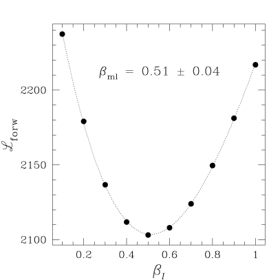
Fig. 8.—: As in the previous figure, now using the 500 km s^-1-smoothed IRAS velocity field predictions. The maximum likelihood values of $\beta_{I}$ differ by very little from those of the previous figure.

The results of applying VELMOD to the expanded sample using 500 km s^-1-smoothed IRAS velocity predictions are shown in Figure 8, in which likelihood for the forward and inverse TF relations is plotted versus $\beta_{I}.$ These runs are carried out using the values of the quadrupole parameters and ${\bf w}_{{\rm LG}}$ obtained from the Paper I 500 km s^-1 run, but again using the modified quadrupole of equation (6) with $R_{Q}=3500\ {\rm km}\,{\rm s}^{-1}.$ We again allow for a density-dependent value of $\sigma_{v};$ we show the results for $\sigma_{v,1}=150\ {\rm km}\,{\rm s}^{-1},$ which maximizes likelihood at 500 km s^-1 smoothing.

The 500 km s^-1 maximum likelihood estimates of $\beta_{I}$ differ little from those obtained at 300 km s^-1 smoothing. Averaging the forward and inverse results, we find $\beta_{I}=0.52\pm 0.05$, only 4% higher than our 300 km s^-1 result. In the VELMOD analysis, the TF data are not smoothed, and therefore we chose a small smoothing scale for the IRAS density field in order to model the velocity field in as much detail as possible. The fact that $\beta_{I}$, and, more significantly, the best values of ${\cal L}_{{\rm forw}}$ and ${\cal L}_{{\rm inv}},$ are essentially unchanged when the smoothing is increased to 500 km s^-1, says that density fluctuations on scales between 300 and 500 km s^-1 contribute little to the velocity field. That is, there is little small-scale power both in the true velocity field, and in the IRAS-predicted velocity field (i.e., the gravity field). The simulations used in the mock catalogs in Paper I do have a substantial amount of small-scale power in the density field, and this is presumably the reason that they yielded a substantially biased estimate of $\beta_{I}$, and a far worse value of ${\cal L}$, with 500 km s^-1 smoothing. Because of the lack of small-scale power in the velocity field, the agreement between our 300 and 500 km s^-1 results for $\beta_{I}$ does not shed light on the question of whether biasing is scale-dependent.

Our 500 km s^-1 runs also detect an increase in the small-scale velocity dispersion with density. For the forward run we find $f_{\delta}=30\ {\rm km}\,{\rm s}^{-1},$ similar to the $300\ {\rm km}\,{\rm s}^{-1}$ value. However, for the inverse run we find $f_{\delta}=60\ {\rm km}\,{\rm s}^{-1}.$ We would expect $f_{\delta}$ to rise with smoothing scale because the density contrasts are generally smaller with larger smoothing. The inverse result confirms this expectation but the forward does not; we do not understand the reason for this difference.

6 VELMOD versus Mark III Catalog TF Calibrations

TABLE 4: VELMOD and Mark III TF Relations^a forward inverse Sample $A$ $b$ $\sigma_{{\rm TF}}$ $D$ $e$ $\sigma_{\eta}$ A82 (VELMOD) $-5.96$ $10.44$ 0.45 $-5.96$ $0.0879$ 0.042 A82 (Mark III) $-5.94$ $10.29$ 0.47 $-5.98$ $0.0893$ 0.043 MAT (VELMOD) $-5.80$ $7.16$ 0.43 $-6.00$ $0.1282$ 0.063 MAT (Mark III) $-5.79$ $6.80$ 0.43 $-5.96$ $0.1328$ 0.059 W91PP (VELMOD) $-4.09$ $7.14$ 0.40 $-4.13$ $0.1217$ 0.052 W91PP (Mark III) $-4.28$ $7.12$ 0.38 $-4.32$ $0.1244$ 0.049 CF (VELMOD) $-4.00$ $8.41$ 0.48 $-3.97$ $0.0948$ 0.049 CF (Mark III) $-4.22$ $7.73$ 0.38 $-4.27$ $0.1190$ 0.047

Table 4:: Notes: (a) Comparison of the VELMOD and Mark III TF calibrations for the four subsamples used in the VELMOD analysis. The typical $1\,\sigma$ errors for both calibrations are: $\delta A=\delta D\simeq 0.03;$ $\delta_{b}/b=\delta e/e=0.03;$ $\delta\sigma_{{\rm TF}}=e^{-1}\delta\sigma_{\eta}=0.02.$

An important feature of VELMOD is that the TF relations for the various samples are determined by maximizing likelihood at each $\beta_{I}.$ The correct TF relations are those obtained for the maximum likelihood value of $\beta_{I},$ which we have found to be $0.50$ with small uncertainty. In Table 4 we give the parameters of the forward and inverse TF relations obtained from our favored VELMOD runs, i.e. 300 km s^-1 smoothing, quadrupole with $R_{Q}=3500\ {\rm km}\,{\rm s}^{-1},$ and density-dependent velocity dispersion with $\sigma_{v,1}=130\ {\rm km}\,{\rm s}^{-1}$ (forward) and $\sigma_{v,1}=110\ {\rm km}\,{\rm s}^{-1}$ (inverse). Columns (1), (2), and (3) list the forward TF parameters $A,$ $b,$ and $\sigma_{{\rm TF}},$ while columns (4), (5), and (6) list the inverse TF parameters $D,$ $e,$ and $\sigma_{\eta}$. Also given in Table 3 are the values of these parameters that went into the Mark III Catalog (Willick et al. 1997a).

The slopes and scatters of the VELMOD and Mark III TF relations are in good agreement overall. The VELMOD MAT TF slope is higher, but by less than $2\,\sigma,$ as we discussed in Paper I, §4.7. The CF slope is higher than its Mark III value, as is its scatter. This is not surprising, because in this paper we have treated CF as a fully independent sample, whereas the Mark III calibration procedure (Willick et al. 1996) assumed that CF had the same TF relation as the Willick (1991) cluster sample, W91CL, up to a slight zero-point adjustment.

More important, there are substantial zero-point differences between the VELMOD and Mark III calibrations. While the VELMOD and Mark III TF zero points of A82 and MAT are in good agreement, those of W91PP and CF differ by about 0.2 mag, for both the forward and inverse TF relations. This difference is much greater than the expected errors of $\sim\,$0.03 mag in either procedure. Because the difference manifests itself for only two of four samples, it cannot arise from a global zero point error in either the Mark III or the VELMOD calibration procedure.

Fig. 9.—: Differences in the radial peculiar velocity inferred from the Mark III and VELMOD forward TF calibrations, plotted as a function of Local Group redshift for the A82 (left panel) and MAT (right panel) samples.

Fig. 10.—: As in the previous figure, for the W91PP (left panel) and CF (right panel) samples.

Figures 9 and 10 show how these differences in the TF parameters translate into peculiar velocity differences. The differences between the Mark III and VELMOD peculiar velocities inferred from the forward TF relation are plotted as a function of LG redshift for each of the four samples. The plots would appear substantially the same if we used inverse TF distances. We do not apply Malmquist bias corrections, which would accentuate the differences between the VELMOD and Mark III velocities. Thus, the TF scatters have no effect on the diagrams.

For A82 there is no meaningful difference between the Mark III and VELMOD inferred peculiar velocities. For MAT, there is a slight trend, but the mean differences are everywhere less than $\sim\,$100 km s^-1, except at the outer edge ($cz\simeq 6000\ {\rm km}\,{\rm s}^{-1}$) of the sample. However, for W91PP and CF the differences are substantial. In each case, the Mark III velocities are more negative by 200–400 km s^-1. In the case of W91PP, the differences are even larger beyond 6000 km s^-1.

This systematic difference between the Mark III and VELMOD TF calibrations has a strong effect on the inferred bulk flow from the Mark III data (cf. Courteau et al. 1993; Dekel 1994; Postman 1995; Strauss 1997, for discussions). The W91PP and CF samples dominate the Northern sky away from the Local Supercluster. W91PP in particular samples the Perseus-Pisces (PP) supercluster, centered at $l\approx 120^{\circ}\,,$ $b\approx-30^{\circ}\,.$ As measured by the Mark III TF calibrations, the PP region is seen as having large, negative radial peculiar velocities in the microwave background frame (e.g., Courteau et al. 1993). This, along with outflowing velocities in the Great Attractor region (traced mainly by the MAT sample), is why measurements of the bulk flow within 6000 km s^-1 from the Mark III data have yielded values in the range $400$–$500\ {\rm km}\,{\rm s}^{-1}$. However, IRAS does not predict strong infall of the PP supercluster region, unless $\beta_{I}$ is $\lower 2.15277pt\hbox{$\,\buildrel<\over{\sim}\,$}0.2.$ Since the VELMOD TF calibrations reflect the IRAS velocity field, they adjust to produce little infall of PP, and thus a much smaller bulk flow, than do the Mark III calibrations.

Another way to state the problem is as follows. The Mark III TF zero points were set by asking for agreement in distances for galaxies in overlapping datasets; the full-sky cluster sample of Han & Mould (1992; HMCL) was the backbone that tied the sky together (cf. Willick et al. 1995, 1996, 1997a). If these calibrations are indeed correct, then the VELMOD calibrations are not, and it follows that the IRAS redshift survey does not correctly predict the peculiar velocity field. In fact, this was the conclusion reached by Davis et al. (1996), whose ITF analysis made use of the Mark III zeropointing procedure even though it did not use the Mark III distances directly. If the IRAS velocity field predictions are correct, as we have assumed in this paper, then so are the VELMOD TF calibrations and our maximum likelihood estimate of $\beta_{I}.$ However, in that case the Mark III TF calibrations are incorrect, and the Mark III Catalog contains erroneous distances for the W91PP and CF samples—and by extension, for the HMCL, W91CL, and elliptical galaxy samples as well. It would then follow that the POTENT peculiar velocity and density fields, which are based on the Mark III distances and were used in the POTIRAS determination of $\beta_{I}=0.89\pm 0.12,$ contain systematic errors. A self-consistent picture would require that the VELMOD TF calibrations, required by the IRAS velocity fields, also be used to produce the POTENT velocity and density maps to estimate $\beta_{I}.$ This has not yet been done.

One can ask whether the VELMOD TF calibrations agree better with the Mark III calibrations for some value of $\beta_{I}$ other than $0.5.$ In fact, for $\beta_{I}=0.1$, the VELMOD W91PP zero point agrees with that of Mark III, for both the forward and inverse TF relations. However, for $\beta_{I}=0.1$ the VELMOD TF zero point for CF is even farther from its Mark III value than it is for $\beta_{I}=0.5.$ For $\beta_{I}\simeq 1,$ the CF zero point is closer to its Mark III value, but the W91PP zero point diverges drastically from Mark III. Also, for very low or very high $\beta_{I}$ we lose the good agreement between the VELMOD and Mark III A82 and MAT TF zero points. Thus there is no value of $\beta_{I}$ at which the VELMOD and Mark III calibrations are in overall agreement.

The question of which set of TF calibrations is correct must ultimately be decided by improved TF data. The problem has arisen because there is no reliable way to tie together the disjoint Southern (MAT) and Northern (CF and W91PP) sky TF data sets that constitute the Mark III field spirals. A82 spans the two hemispheres but is dominated by nearby galaxies and has little overlap with the Northern sky samples. The HMCL sample was thought to provide the needed overlap, but its uniformity across the sky has been called into question by the calibration disrepancies. What is needed are homogeneous TF data that cover the celestial sphere. In collaboration with S. Courteau, M. Postman, and D. Schlegel, we have obtained uniform TF data for $\sim\,$300 galaxies isotropically distributed in the spherical shell defined by $4500\lower 2.15277pt\hbox{$\,\buildrel<\over{\sim}\,$}cz\lower 2.15277pt\hbox{$\,\buildrel<\over{\sim}\,$}7000\ {\rm km}\,{\rm s}^{-1}.$ Reduction of these data are under way, and results are expected by late 1998. Comparison of these uniform TF data with the Mark III data will allow a definitive resolution of the calibration problem.

Finally, we note that adopting the Mark III TF calibrations has relatively little effect on the maximum likelihood $\beta_{I}$ obtained from VELMOD. With the $300\ {\rm km}\,{\rm s}^{-1}$-smoothed IRAS plus quadrupole velocity model, we obtain $\beta_{I}=0.44$ (forward) and $\beta_{I}=0.45$ (inverse) when the TF parameters for all four samples are fixed to their Mark III values as given in Table 4. For the no-quadrupole model we obtain $\beta_{I}=0.50$ (forward) and $\beta_{I}=0.51$ (inverse). The likelihoods obtained from these VELMOD runs are, of course, much worse (by $\sim\,$100 units in ${\cal L}$) than for our preferred runs in which the twelve TF parameters are free. Thus, while the TF calibration problem is crucial for the match of the IRAS velocity field to the TF data, as we discuss in the next section, it is secondary for the determination of $\beta_{I}.$

7 The Goodness of Fit of the IRAS Velocity Field

Although VELMOD does not produce a picture of the TF velocity field, we can nonetheless use it to visualize how well the TF data fit the IRAS velocity predictions. We do so by converting the VELMOD apparent magnitude $m$ (forward) or velocity width parameter $\eta$ (inverse) residuals into smoothed radial peculiar velocity residuals with respect to IRAS, as described in Paper I, § 5.1. The VELMOD residuals also enable us to measure the goodness of fit of the velocity model, as we describe below. The smoothed peculiar velocity residual is given by equation 24 of Paper I:

$$\delta u_{i}^{s}=d_{i}\left[1-f_{i}10^{0.2(\delta_{m,i}^{s}\times\Delta m_{i})}\right]\,,$$ (9)

which we repeat here because of a typographical error in Paper I; see Paper I for the definition of the various symbols in this equation.

Figures 11, 12, and 13 show sky maps of these velocity residuals for $\beta_{I}=0.5,$ $\beta_{I}=0.1,$ and $\beta_{I}=1.0$ respectively. In each case, the results are based on forward TF residuals from our preferred 300 km s^-1 smoothing run (see the notes to Table 3). Open symbols represent negative velocity residuals (i.e., the TF distance to the object is greater than that predicted by IRAS); starred symbols represent positive velocity residuals. The Gaussian smoothing scale for the maps is given by $250\left[1+(cz_{{\rm LG}}/2500)^{2}\right]^{1/2}\ {\rm km}\,{\rm s}^{-1}.$ Thus, the smoothing radius varies from 250 km s^-1 nearby to $\sim\,$750 km s^-1 at the edge of the sample. This smoothing imposes a coherence scale of $\sim\,$15–25${}^{\circ}\,$ on the results; patches this size with similar velocity residuals are to be expected in the maps from the smoothing alone, while any coherence seen on much larger scales represents a real error in the model. Points are plotted only for galaxies which have enough near neighbors to allow an adequate smoothing; this is why there are few galaxies represented in the Northern Galactic Cap at $cz>2500\ {\rm km}\,{\rm s}^{-1},$ where the sampling is very dilute. Such points, if plotted, would exhibit large velocity residuals due solely to TF scatter and would not help us assess the quality of the fit.

Inspection of these maps shows clearly why $\beta_{I}=0.5$ is the best fit. Although there is some real excess coherence to the residuals (we discuss this further below), the coherent velocity levels are generally at a low level ($\lower 2.15277pt\hbox{$\,\buildrel<\over{\sim}\,$}250\ {\rm km}\,{\rm s}^{-1}$). There are many alternating regions of positive and negative residuals, showing that globally at least the residual map is fairly incoherent. This is what is required of a good fit. There are no extended regions where the velocity residuals are consistently greater than 300 km s^-1. This is a qualitative indication that the IRAS plus quadrupole velocity field model fits the major features of the actual velocity field. As in Paper I, coherent residuals are present when the quadrupole is not modeled. That being said, with $R_{Q}=3500\ {\rm km}\,{\rm s}^{-1}$, the quadrupole contribution at $cz\lower 2.15277pt\hbox{$\,\buildrel>\over{\sim}\,$}5000\ {\rm km}\,{\rm s}^{-1}$ is negligible. Thus, the good agreement on very large scales is due to the IRAS velocity field alone, giving a posteriori confirmation of our quadrupole model.

The residual maps produced at $\beta_{I}=0.1$ and at $\beta_{I}=1.0,$ on the other hand, show considerable coherence. Moreover, the amplitude of the velocity residuals in these regions is often large, $\lower 2.15277pt\hbox{$\,\buildrel>\over{\sim}\,$}300\ {\rm km}\,{\rm s}^{-1}.$ Low and high $\beta_{I}$ are clearly worse fits to the TF data than is $\beta_{I}=0.5.$ The maps, then, confirm what the likelihood analysis is telling us. It is important to remember that the poor fit at low and high $\beta_{I}$ is not a result of errors in the assumed TF relation, for the TF relations used were those preferred by the data at each $\beta_{I}$. The poor fit is a genuine reflection of the incorrectness of the IRAS velocity field for low and high $\beta_{I}.$

Fig. 11.—: Smoothed VELMOD velocity residuals plotted in Galactic coordinates, for $\beta_{I}=0.5.$ Open circles indicate objects inflowing relative to the velocity model, while starred symbols represent outflowing objects. The symbol size indicates the magnitude of the velocity residual, as coded at the lower right of each plot.

Fig. 12.—: Same as the previous figure, but for $\beta_{I}=0.1.$

Fig. 13.—: Same as the previous figure, but for $\beta_{I}=1.0.$

Fig. 14.—: VELMOD residual autocorrelations, $\psi(\tau)$, plotted for $\beta_{I}=0.5,$ $\beta_{I}=0.1,$ and $\beta_{I}=1.0.$ Nonzero values of $\psi(\tau)$ indicate coherence of the TF versus IRAS residuals on a spatial scale $\tau.$ Such coherence is pronounced for $\beta_{I}=0.1$ and $\beta_{I}=1.0,$ indicating a poor fit. It is insignificant for $\beta_{I}=0.5.$

We may quantify our visual impressions by means of the residual autocorrelation function $\psi(\tau),$ defined by equation (25) of Paper I. In Figure 14, we plot $\psi(\tau)$ for the three values of $\beta_{I}$ represented in the previous figures. The plots show that for $\beta_{I}=0.1$ and $\beta_{I}=1.0,$ significant excess correlation is evident on small and large scales. At $\beta_{I}=0.5,$ the $\psi(\tau)$ is consistent with zero on all scales. There is a small amount of positive correlation on scales $\lower 2.15277pt\hbox{$\,\buildrel<\over{\sim}\,$}2500\ {\rm km}\,{\rm s}^{-1}$ for $\beta_{I}=0.5,$ consistent with the (low-amplitude) inflowing monopole residuals in the upper panel of Figure 11. This may be indicative of a breakdown of the IRAS model at some level, but it is not highly significant, as we now show.

Fig. 15.—: The residual correlation statistic $\chi^{2}_{\xi},$ plotted as a function of $\beta_{I}.$ The heavy line shows the expectation value of this statistic; the dot-dashed and dashed lines show the $1\,\sigma$ and $3\,\sigma$ deviations respectively.

A rigorous measure of the level of residual coherence comes through the use of the correlation $\chi^{2}$ statistic, $\chi^{2}_{\xi},$ defined by equation (26) of Paper I. We plot $\chi^{2}_{\xi}$ versus $\beta_{I}$ in Figure 15. (The value for $\beta_{I}=0.1$ is off-scale.) In Paper I we showed that this statistic had properties similar to that of a true $\chi^{2}$ statistic, but with a mean of $0.87\pm 0.06$ per degree of freedom rather than unity. Its variance was consistent with that of a true $\chi^{2}$ statistic. We indicate the expected value of $\chi^{2}_{\xi}$ (in this case, 63.5 for 73 degrees of freedom) as a heavy solid line on the plot. The 1- and $3\,\sigma$ deviations from the expectation are indicated as dot-dashed and dashed lines, respectively. The quantity $\chi^{2}_{\xi}$ reaches its minimum at the maximum likelihood value of $\beta_{I}.$ The only other value of $\beta_{I}$ for which $\chi^{2}_{\xi}$ is within $3\sigma$ of the expectation value is $\beta_{I}=0.6.$ $\beta_{I}\leq 0.4$ and $\beta_{I}\geq 0.7$ are ruled out at the $>3\,\sigma$ level.

8 Summary

We have applied the VELMOD method to a TF sample drawn from the Mark III Catalog in order to estimate $\beta_{I}=\Omega^{0.6}/b_{I},$ where $b_{I}$ is the linear biasing parameter for IRAS galaxies. The TF sample consists of 1876 galaxies, comprising nearly all Mark III field spirals to a limiting redshift of $cz_{{\rm LG}}=7500\ {\rm km}\,{\rm s}^{-1}.$ This analysis extends the one we presented in Paper I, which was limited to 838 galaxies with $cz_{{\rm LG}}\leq 3000\ {\rm km}\,{\rm s}^{-1}.$ As in Paper I, peculiar velocities were predicted from galaxy density contrasts obtained from the IRAS 1.2 Jy redshift survey (Fisher et al. 1995), under the assumption of linear gravitational instability theory and linear biasing. We developed an analytic approximation to the single-object VELMOD likelihoods, applicable to $\lower 2.15277pt\hbox{$\,\buildrel>\over{\sim}\,$}75\%$ of sample objects, which makes the code run 3–4 times faster.

We carried out the VELMOD analysis using both the forward and inverse forms of the TF relation. Consistency between the two is required to ensure that selection biases are unimportant. We found that the maximum likelihood values of $\beta_{I},$ as well as other important velocity parameters, were indeed statistically the same for both forms of the TF relation. In addition, we allowed the quadrupole velocity residual detected in Paper I to cut off smoothly beyond a radius, $R_{Q},$ whose value we determined through likelihood maximization to be $3500\pm 1000\ {\rm km}\,{\rm s}^{-1}.$ There is little covariance between $R_{Q}$ and $\beta_{I}$. We believe the quadrupole is real and readily accounted for (cf. Paper I, Appendix B). We may summarize our results as $\beta_{I}=0.50\pm 0.04\pm 0.04,$ where the first errorbar is statistical and the second is systematic. This value is quoted for our favored model in which the IRAS densities are smoothed with a 300 km s^-1 Gaussian, the small-scale velocity dispersion varies with density (see below), and in which the quadrupole, with $R_{Q}=3500\ {\rm km}\,{\rm s}^{-1},$ is added to the IRAS-predicted velocity field. The systematic error is due to the quadrupole; if it is not valid to add it, we obtain $\beta_{I}=0.53\pm 0.04$ (forward), or $\beta_{I}=0.54\pm 0.04$ (inverse). We also found that changing the IRAS smoothing scale from 300 to 500 km s^-1 does not significantly affect the derived value of $\beta_{I}.$ This implies that there is little contribution to the velocity and gravity fields from fluctuations on scales between 300 and 500 km s^-1. Further work needs to be done to quantify this, and to understand what effect our Wiener filter, which suppresses fluctuations at large distances, might have on this result.

We tested for a density-dependence of the small-scale velocity dispersion, by modeling a linear variation of $\sigma_{v}$ with the galaxy density contrast $\delta_{g}$ and determining the coefficient through likelihood maximization. This significantly improved the VELMOD likelihood, with a best fit relation $\sigma_{v}=[(100\pm 25)+35\,\delta_{g}]\ {\rm km}\,{\rm s}^{-1}.$ This confirms and strengthens our Paper I result that the galaxy velocity field is remarkably cold. Our detection of an increase in $\sigma_{v}$ with density agrees qualitatively with the results of Strauss et al. (1998), but our coefficient of $\delta_{g}$ is considerably smaller than their value of $\sim\,$50–100 km s^-1.

We showed that the IRAS-predicted velocity field, with quadrupole, is a good fit to the TF data; the correlation function of velocity residuals at $\beta_{I}=0.5$ is consistent with zero on all scales. Strong velocity residual correlations on both small and large scales are seen for $\beta_{I}\leq 0.4$ and $\beta_{I}\geq 0.7,$ indicating that the IRAS-predicted velocity field is not a good fit for these values of $\beta_{I}.$ Davis et al. (1996), who adopted the Mark III TF zero points, found highly significant discrepancies between the IRAS-predicted and Mark III-observed velocity fields at all $\beta_{I}.$ The VELMOD procedure requires no a priori calibration of the TF relation, and with this freedom, the IRAS-predicted velocity field matches the TF data well, suggesting that the Davis et al. (1996) discrepancies are tied to uncertainties in the TF calibrations. Our claim of agreement between the predicted and observed velocity fields can hold up only if the VELMOD TF calibrations ultimately prove correct.

Indeed, we showed by direct comparison of TF parameters that the VELMOD and Mark III TF calibrations (Willick et al. (1997a) differ significantly. The VELMOD TF relations for CF and W91PP yield distances $\sim\,$8% shorter than the Mark III TF calibrations, whereas the VELMOD and Mark III TF calibrations for A82 and MAT are in good agreement. This has a strong effect on the large-scale bulk flow inferred from the data. The VELMOD TF calibrations cannot be brought into closer agreement with the Mark III calibration by changing $\beta_{I},$ or by an overall zero point shift in all TF samples. If the VELMOD TF relations are correct, then the overall Mark III TF calibration cannot be. Analyses based on the published Mark III distances should thus be interpreted with caution.

The VELMOD TF calibrations are valid, however, only to the degree that the IRAS-predicted peculiar velocities are accurate. This will be the case provided that IRAS galaxies trace mass up to linear biasing, and linear gravitational instability theory is a good approximation when the galaxy densities are smoothed on a 300–500 km s^-1 Gaussian scale. Ultimately, the calibration issue must be settled by improved observational data. We are carrying out a full-sky TF for this purpose, and will report the results of this effort in 1–2 years.

Our result $\beta_{I}\simeq 0.5$ is virtually unchanged from Paper I, ruling out the possibility that cosmic scatter and the small volume studied biased our Paper I $\beta_{I}.$ Thus, this paper sharpens the discrepancy between the VELMOD measurement of $\beta_{I}$ and that obtained from the POTIRAS comparison, $\beta_{I}\simeq 0.89\pm 0.12$ (Sigad et al. 1998). Further underscoring this discrepancy are two analyses that have appeared since Paper I, that of Riess et al. (1997) who find $\beta_{I}=0.4\pm 0.15$ using SN Ia as tracers of the velocity field, and that of da Costa et al. (1997) who found $\beta_{I}=0.6\pm 0.12$ using the SFI TF data set. It may be that the differences in the derived values of $\beta_{I}$ center on whether the comparison is done at the level of the velocities (the $v$-$v$ comparison, as in this paper, Riess et al., and da Costa et al.) or at the level of the densities (the $d$-$d$ comparison, as in POTIRAS). Future work is needed to determine whether these differences can be explained in terms of physical effects, such as a scale-dependent biasing relation (e.g., Sigad et al. 1998), or whether they result from TF calibration errors, as discussed above, or other methodological factors. The question is an important one because the values of $\beta_{I}$ obtained from the $v$-$v$ analyses favor a low-density ($\Omega=0.2$–$0.5$) universe, while the POTIRAS $\beta_{I}$ is suggestive of an $\Omega=1$ cosmology, if $b_{I}\lower 2.15277pt\hbox{$\,\buildrel<\over{\sim}\,$}1,$ as suggested by recent analyses of the evolution of rich clusters (Bahcall, Fan, & Cen 1997; Fan, Bahcall, & Cen 1997).

A Appendix: Derivation of Approximate Likelihoods

The full expressions for the VELMOD likelihoods are given by equations 11 and 12 of Paper I:

$$P(m|\eta,cz)=\frac{\int_{0}^{\infty}\!dr\,r^{2}n(r)\,P(cz|r)\,S(m,\eta,r)\exp\!\left(-\frac{\left[m-(M(\eta)+\mu(r))\right]^{2}}{2\sigma_{{\rm TF}}^{2}}\right)}{\int_{0}^{\infty}\!dr\,r^{2}n(r)\,P(cz|r)\,\int_{-\infty}^{\infty}\!dm\,S(m,\eta,r)\exp\!\left(-\frac{\left[m-(M(\eta)+\mu(r))\right]^{2}}{2\sigma_{{\rm TF}}^{2}}\right)}\,;$$ (A1)

$$P(\eta|m,cz)=\frac{\int_{0}^{\infty}\!dr\,r^{2}n(r)\,\Phi(m-\mu(r))\,P(cz|r)\,S(m,\eta,r)\exp\!\left(-\frac{\left[\eta-\eta^{0}(m-\mu(r))\right]^{2}}{2\sigma_{\eta}^{2}}\right)}{\int_{0}^{\infty}\!dr\,r^{2}n(r)\,\Phi(m-\mu(r))\,P(cz|r)\,\int_{-\infty}^{\infty}\!d\eta\,S(m,\eta,r)\exp\!\left(-\frac{\left[\eta-\eta^{0}(m-\mu(r))\right]^{2}}{2\sigma_{\eta}^{2}}\right)}\,,$$ (A2)

where

$$P(cz|r)=\frac{1}{\sqrt{2\pi}\,\sigma_{v}}\exp\!\left(-\frac{[cz-(r+u(r))]^{2}}{2\sigma_{v}^{2}}\right)\,,$$ (A3)

$S(m,\eta,r)$ is the selection function, and $\mu(r)\equiv 5\log r$ is the distance modulus. Note the typographical error in equation 11 of Paper I; equation (A1) is correct. In this Appendix, we derive analytic approximations to equations (A1) and (A2) using the method of steepest descent. We first consider the simple case of no selection ($S=1$) in A.1, and then consider distance-independent selection functions (A.2). The MAT sample selection function does have a distance dependence; we treat this case in A.3. In A.4 we further refine the approximation and summarize results.

A.1 The Case of No Selection

Equation (A3) gives the probability that an object at distance $r$ exhibits redshift $cz.$ That probability is greatest for $r=w,$ where $w$ is the “crossing point” defined implicitly by $cz=w+u(w)$. Expanding about the crossing point gives $[cz-(r+u(r))]\approx-(r-w)(1+u^{\prime}),$ where $u^{\prime}$ is the radial peculiar velocity derivative at the crossing point. To the same order of approximation we may write $(r-w)\approx w\ln(r/w).$ With these approximations, equation (A3) becomes:

$$P(cz|r)=\frac{1}{\sqrt{2\pi}\sigma_{v}}\,\exp\left(-\frac{\ln(r/w)^{2}}{2\Delta_{v}^{2}}\right)\,,$$ (A4)

where $\Delta_{v}\equiv\sigma_{v}/[w(1+u^{\prime})].$

This approximation is valid under certain conditions: First, there must be a unique crossing point $w.$ Second, $u(r)$ must be adequately linear within a few times $\sigma_{v}$ of $w.$ Third, $w$ must be sufficiently large that the approximation $(r-w)/w\approx\ln(r/w)$ is a good one for $r$ within a few times $\sigma_{v}$ of $w$. The second and third conditions are satisfied when $\Delta_{v}\ll 1;$ in practice we found that $\Delta_{v}\leq 0.2$ was usually sufficient to ensure good accuracy (after the refinements discussed in § A.4).

We consider first the forward TF likelihood, equation (A1), in the case of no sample selection ($S=1$). Substituting equation (A4) into equation (A1) gives

$$P(m|\eta,cz)=\frac{\int_{0}^{\infty}dr\,r^{2}n(r)\exp\left(-\frac{\ln(r/w)^{2}}{2\Delta_{v}^{2}}\right)\exp\left(-\frac{\ln(r/d)^{2}}{2\Delta_{{\rm TF}}^{2}}\right)}{\sqrt{2\pi}\sigma_{{\rm TF}}\int_{0}^{\infty}dr\,r^{2}n(r)\exp\left(-\frac{\ln(r/w)^{2}}{2\Delta_{v}^{2}}\right)}$$ (A5)

where $\Delta_{{\rm TF}}\equiv\frac{\ln 10}{5}\sigma_{{\rm TF}}$ and $d$ is the forward TF distance (§ 2.3). The integrals in equation A5 can be evaluated analytically if we assume that the density field behaves locally as a power law,

$$n(r)=n(w)\left(\frac{r}{w}\right)^{\gamma}\,.$$ (A6)

In practice, $n(r)$ is not a true power law and the exponent is evaluated as $\gamma(w)=\left[d\ln n(r)/d\ln r\right]_{r=w}.$ With this assumption, equation A5 may be written

$$P(m|\eta,cz)=\frac{\int_{-\infty}^{\infty}e^{(3+\gamma)x}e^{-\frac{x^{2}}{2\Delta_{v}^{2}}}e^{-\frac{(x-y)^{2}}{2\Delta_{{\rm TF}}^{2}}}dx}{\sqrt{2\pi}\sigma_{{\rm TF}}\int_{-\infty}^{\infty}e^{(3+\gamma)x}e^{-\frac{x^{2}}{2\Delta_{v}^{2}}}dx}\,.$$ (A7)

where $x\equiv\ln(r/w)$ and $y\equiv\ln(d/w).$ The numerator and denominator integrals of equation (A7) may be straightforwardly evaluated to obtain

$$P(m|\eta,cz)=\frac{\ln 10}{5}\frac{1}{\sqrt{2\pi}\,\Delta_{e}}\,\exp\left\{-\frac{1}{2\Delta_{e}^{2}}\left(y-(3+\gamma)\Delta_{v}^{2}\right)^{2}\right\}\,,$$ (A8)

where

$$\Delta_{e}\equiv\left[\Delta_{{\rm TF}}^{2}+\Delta_{v}^{2}\right]^{1/2}\,.$$ (A9)

Equation (A8) has a simple interpretation. When sample selection is neglected, the TF distance $d$ is log-normally distributed; the expectation value of $\ln d$ is $\ln w+(3+\gamma)\Delta_{v}^{2}.$ The fact that $E(\ln d)\neq\ln w$ is due to the Malmquist bias associated with velocity noise; there is both a homogeneous ($3\Delta_{v}^{2}$) and an inhomogeneous ($\gamma\Delta_{v}^{2}$) term. Unlike the Malmquist bias in a Method I approach which scales as $\Delta_{{\rm TF}}^{2}$ (cf. SW), the bias here is proportional to $\Delta_{v}^{2}\propto(\sigma_{v}/w)^{2},$ which is generally much smaller, and which decreases with distance.

The expression for the inverse probability, equation (A2), is complicated by the presence of the luminosity function $\Phi$ in both numerator and denominator. However, like the density field, this function varies slowly on the scale relevant to the integration. Consequently, we may treat it too as a power law for $r$ near $w:$

$$\Phi(m-\mu(r))\approx\Phi(m-\mu(w))\left(\frac{r}{w}\right)^{\lambda}\,.$$ (A10)

Again, we evaluate the power-law exponent according to $\lambda(w)\equiv\left\{d\ln[\Phi(m-\mu(r))]/d\ln r\right\}_{r=w}.$ Once this is done, the integrals simplify in the same way as for the forward relation, and we find after similar manipulations

$$P(\eta|m,cz)=\frac{\ln 10}{5}\frac{1}{e}\frac{1}{\sqrt{2\pi}\,\Delta_{e,{\rm inv}}}\,\exp\left\{-\frac{1}{2\Delta_{e,{\rm inv}}^{2}}\left(y_{{\rm inv}}-(3+\gamma+\lambda)\Delta_{v}^{2}\right)^{2}\right\}\,.$$ (A11)

Here $y_{{\rm inv}}\equiv\ln(d_{{\rm inv}}/w),$ where $d_{{\rm inv}}$ is the inverse TF distance and $e$ is the inverse TF slope (§ 2.3). The fractional inverse TF distance error is given by

$$\Delta_{e,{\rm inv}}\equiv\left[\Delta_{\eta}^{2}+\Delta_{v}^{2}\right]^{1/2}$$ (A12)

where $\Delta_{\eta}\equiv(\ln 10/5)\sigma_{\eta}/e.$

Comparison of Eqs. A8 and A11 reveals the close analogy between the forward and inverse probability expressions when selection is neglected. Such an analogy must indeed hold, for the two forms of the TF relation contain the same information. The factor $e^{-1}$ in equation A11 simply renormalizes the probability density to $\eta$-space, while the $\lambda$ reflects the luminosity function dependence of the inverse expression.

A.2 The role of selection

In this section, we assume that the sample selection function has no explicit $r$-dependence, i.e., $S=S(m,\eta).$ We assume the sample to be selected on a quantity $\xi$ with limiting value $\xi_{\ell}$, which is linearly related to the TF observables:

$$\xi(m,\eta)=a_{1}-b_{1}m-c_{1}\eta\qquad\hbox{with scatter $\sigma_{\xi}$}\,.$$ (A13)

The quantities $a_{1},$ $b_{1},$ and $c_{1}$ and $\sigma_{\xi}$ were determined empirically for the Mark III samples by Willick et al. (1995, 1996). Willick (1994) shows that:

$$S(m,\eta)=\frac{1}{2}\left[1+{\rm erf}({\cal A}_{\xi}(m,\eta)\right]\,,$$ (A14)

where

$${\cal A}_{\xi}(m,\eta)\equiv\frac{\xi(m,\eta)-\xi_{\ell}}{\sqrt{2}\sigma_{\xi}}\,.$$ (A15)

We define a TF-predicted apparent magnitude $m_{r}\equiv M(\eta)+5\log r$. Then, using the identities derived by Willick (1994), the forward likelihood becomes:

$$P(m|\eta,cz)=\frac{\left[1+{\rm erf}({\cal A}_{\xi}(m,\eta))\right]}{\sqrt{2\pi}\sigma_{{\rm TF}}}\frac{\int r^{2}n(r)P(cz|r)\exp\left(-\frac{\ln(r/d)^{2}}{2\Delta_{{\rm TF}}^{2}}\right)\,dr}{\int r^{2}n(r)P(cz|r)\left[1+{\rm erf}\left({\cal A}_{\xi}(m_{r},\eta)/\sqrt{1+\beta^{2}}\right)\right]\,dr}\,,$$ (A16)

where $\beta\equiv b_{1}\sigma_{{\rm TF}}/\sigma_{\xi}.$

The integral over $m$ has caused the ${\cal A}_{\xi}$ term in the deonominator to acquire an $r$-dependence, although it did not start out with one. This complication makes it inconvenient to follow our previous procedure exactly. Instead, we treat this term as constant across the effective range of integration, and take it outside the integral; this is correct to the same order of approximation. This leaves us with a ratio of integrals we have already evaluated. We then require that the resultant probability density $P(m|\eta,cz)$ be properly normalized, yielding:

$$P(m|\eta,cz)=\frac{\ln 10}{5}\frac{1+{\rm erf}\left[{\cal A}_{\xi}(m,\eta)\right]}{1+{\rm erf}\left[\frac{{\cal A}_{\xi}(m_{0},\eta)}{\sqrt{1+\beta^{2}}}\right]}\frac{1}{\sqrt{2\pi}\,\Delta_{e}}\exp\left\{-\frac{1}{2\Delta_{e}^{2}}\left(y-(3+\gamma)\Delta_{v}^{2}\right)^{2}\right\}\,,$$ (A17)

where

$$m_{0}(\eta,w)\equiv M(\eta)+5\log w+\frac{5}{\ln 10}\left[3+\gamma\right]\Delta_{v}^{2}$$ (A18)

and

$$\beta\equiv\frac{b_{1}\sigma_{e}}{\sigma_{\xi}}\qquad{\rm where\ }\sigma_{e}\equiv 5\Delta_{e}/\ln 10\,.$$ (A19)

The effect of selection appears purely outside the exponent now. Indeed, the role of selection is very similar to what it was in pure Method II (Willick 1994), with a slightly different evaluation of ${\cal A}_{\xi}$ and $\beta$ in the denominator.

The corresponding expression for the inverse relation follows directly, given the analogy we drew between the two expressions in the previous subsection:

$$P(\eta|m,cz)=\frac{\ln 10}{5}\,e^{-1}\frac{1+{\rm erf}\left[{\cal A}_{\xi}(m,\eta)\right]}{1+{\rm erf}\left[\frac{{\cal A}_{\xi}(m,\eta_{0})}{\sqrt{1+\beta^{2}}}\right]}\frac{1}{\sqrt{2\pi}\,\Delta_{e}}\exp\left\{-\frac{1}{2\Delta_{e}^{2}}\left(y-(3+\gamma+\lambda)\Delta_{v}^{2}\right)^{2}\right\}\,,$$ (A20)

where

$$\eta_{0}(m,w)\equiv\eta^{0}\left(m-\left[5\log w+\frac{5}{\ln 10}(3+\gamma+\lambda)\Delta_{v}^{2}\right]\right)$$ (A21)

and

$$\beta\equiv\frac{c_{1}\sigma_{\eta,e}}{\sigma_{\xi}}\qquad{\rm where\ }\sigma_{\eta,e}\equiv\sqrt{\sigma_{\eta}^{2}+\left(5e/\ln 10\Delta_{v}\right)^{2}}\,.$$ (A22)

Note the different definition of $\beta$ in the inverse and forward cases. In particular, if selection is $\eta$-independent ($c_{1}=0$), the terms involving the error functions cancel, and $P(\eta|m,cz)$ reduces to the no selection case, as expected.

A.3 Treating an explicitly distance-dependent selection function

If the selection function $S$ has an explicit distance dependence, things get a bit more complicated. In Willick et al. (1996), the data for all the Mark III samples was fit to the form,

$$\xi=\xi(m,\eta,r)=a_{1}-b_{1}m-c_{1}\eta-d_{1}\log r\,;$$ (A23)

only MAT had a significantly non-zero value of $d_{1}$. However, $c_{1}=0$ for MAT; selection for MAT has no explicit $\eta$-dependence and we take this into account in what follows. Corresponding to equation (A23) is an $r$-dependent ${\cal A}_{\xi}$ parameter,

$${\cal A}_{\xi}(m,r)\equiv\frac{\xi(m,r)-\xi_{\ell}}{\sqrt{2}\sigma_{\xi}}\,,$$ (A24)

and thus the selection function $S(m,r)=\left[1+{\rm erf}({\cal A}_{\xi}(m,r)\right]/2.$

The main effect of distance-dependent selection is to introduce a new power-law exponent, $\alpha,$ into our earlier expressions, where

$$\alpha(m,w)\equiv\left.\frac{d\ln S}{d\ln r}\right|_{r=w}=-\sqrt{\frac{2}{\pi}}\frac{d_{1}}{\ln 10\,\sigma_{\xi}}\frac{e^{-{\cal A}_{\xi}^{2}}}{\left[1+{\rm erf}({\cal A}_{\xi})\right]}\,.$$ (A25)

For the inverse relation, the addition of $\alpha$ is all that is required to correct our expressions. Specifically,

$$P(\eta|m,cz)=\frac{\ln 10}{5}\frac{1}{e}\frac{1}{\sqrt{2\pi}\,\Delta_{e,inv}}\,\exp\left\{-\frac{1}{2\Delta_{e,inv}^{2}}\left(y_{inv}-(3+\gamma+\lambda+\alpha)\Delta_{v}^{2}\right)^{2}\right\}\,,$$ (A26)

There are no selection functions out in front because for MAT, selection is $\eta$-independent.

For the forward relation, the fact that $\alpha$ depends on $m$ ruins the pure Gaussianity of the exponent. Using the same approach as we did to derive equation (A17), we assume that $\alpha$ varies slowly with $m$, take ${\cal A}_{\xi}$ out of the denominator integral, and normalize after the fact. After some algebra, one finds

$$P(m|\eta,cz)\simeq\frac{\ln 10}{5}\,\frac{1+{\rm erf}\left({\cal A}_{\xi}(m,w)\right)}{1+{\rm erf}\left[\frac{{\cal A}_{\xi}(\overline{m},w)}{\sqrt{1+\beta^{2}}}\right]}\,\frac{1}{\sqrt{2\pi}\,\Delta_{e}^{\prime}}\,\exp\left\{-\frac{1}{2\Delta_{e}^{2}}\left(y-(3+\gamma+\alpha(m,w))\Delta_{v}^{2}\right)^{2}\right\}\,.$$ (A27)

In equation A27, the individual terms have the following definitions:

$$\overline{m}\equiv m_{0}+\alpha(m_{0},w)\frac{5}{\ln 10}\Delta_{v}^{2}\,,$$ (A28)

$$\Delta_{e}^{\prime}\equiv\Delta_{e}\left[1-{{5}\over{\ln 10}}\Delta_{v}^{2}{{d\alpha}\over{dm}}\right]^{-1}=\Delta_{e}\left[1-{{5\sqrt{2}\,b_{1}\alpha(m,w)\Delta_{v}^{2}}\over{\ln 10\,\sigma_{e}}}\left({\cal A}_{\xi}-{{\alpha(m,w)\ln 10\,\sigma_{\xi}}\over{\sqrt{2}\,d_{1}}}\right)\right]^{-1}$$ (A29)

$$\beta\equiv\frac{b_{1}\sigma_{e}^{\prime}}{\sigma_{\xi}}\qquad{\rm where\ }\sigma_{e}^{\prime}\equiv{{5\Delta_{e}^{\prime}}\over{\ln 10}}\,.$$ (A30)

A.4 Final Refinement and Summary

Our original approximation to $P(cz|r)$, equation (A4), was correct to first order in $\sigma_{v}.$ This leads to systematic inaccuracies in two regimes: small distances ($\lower 2.15277pt\hbox{$\,\buildrel<\over{\sim}\,$}2000\ {\rm km}\,{\rm s}^{-1}$), where the approximation $(r-w)/w\approx\ln(r/w)$ loses accuracy, and in regions of velocity field curvature, when $u^{\prime\prime}\sigma_{v}$ is comparable to $u^{\prime}.$ We extend its regime of validity by making second-order corrections for these effects.

To second order in $x\equiv\ln(r/w)$ we find $(r-w)/w=x+x^{2}/2$. Using this and a second order Taylor expansion of $u(r)$ about $w,$ and retaining only terms of order $(\sigma_{v}/w)^{2}$ in the exponent, we find after some algebra

$$\exp\left[-\frac{1}{2\sigma_{v}^{2}}\left(cz-[r+u(r)]\right)^{2}\right]=e^{-x^{2}/2\Delta_{v}^{2}}\times f(r)\,,$$ (A31)

where

$$f(r)\equiv e^{(1+\varepsilon)\,x^{3}/2\Delta_{v}^{2}}\ ,\ \varepsilon\equiv\frac{u^{\prime\prime}w}{1+u^{\prime}}\,,$$ (A32)

where $u^{\prime}$ and $u^{\prime\prime}$ are evaluated at $w.$ The term $e^{-x^{2}/2\Delta_{v}^{2}}$ in equation (A31) is just our original approximation for $P(cz|r),$ equation (A4), and $f(r)$ is the second-order correction. It is non-Gaussian in $\ln(r/w)$ and thus cannot be analytically integrated as before.

We thus treat it as we have other slowly-varying terms: we approximate it as a power law in the vicinity of the crossing point. However, because of its cubic nature, the local logarithmic derivative is identically zero. We thus proceed heuristically by calculating the power-law exponent as a finite difference over an interval of $\ln r$ of $\pm g\Delta_{v}$, where $g$ is of order unity:

$$\nu\sim\frac{\ln f(x=g\Delta_{v})-\ln f(x=-g\Delta_{v})}{2\,g\Delta_{v}}=-\frac{g^{2}}{2}\left(1+\varepsilon\right)$$ (A33)

We calibrated the appropriate value of $g$ by varying it until we maximized agreement between the exact and approximate likelihoods. This happened at $g=1.5,$ and thus the correct exponent is

$$\nu=-1.1\left(1+\varepsilon\right)\,.$$ (A34)

This leads to the final forms of the analytic approximation to the VELMOD likelihoods. For the forward relation, $P(m|\eta,cz)$ is given by equation (A17) for A82, W91PP, and CF (the samples for which the selection function has no explicit distance dependence) and by equation (A27) for MAT. For the inverse relation, $P(\eta|m,cz)$ is given by equation (A20) for A82, W91PP, and CF and by equation (A26) for MAT. However, in all of these equations, the quantity $3+\gamma$ is replaced by $3+\gamma+\nu,$ where $\nu$ is given by equation (A34), and $\varepsilon$ is given by equation (A32). Note that the definition of $\nu$ is such that the homogeneous Malmquist bias term is reduced from $3\Delta_{v}^{2}$ to $1.9\Delta_{v}^{2}.$ This is a significant effect for distances $\lower 2.15277pt\hbox{$\,\buildrel<\over{\sim}\,$}2000\ {\rm km}\,{\rm s}^{-1},$ and thus the refinement discussed here is crucial for extending the regime of validity of the approximation to small distances.