Excursion set approach to the clustering of dark matter haloes in Lagrangian space

Abstract

We present a stochastic approach to the spatial clustering of dark matter haloes in Lagrangian space. Our formalism is based on a local formulation of the ‘excursion set’ approach by Bond et al., which automatically accounts for the ‘cloud-in-cloud’ problem in the identification of bound systems. Our method allows to calculate correlation functions of haloes in Lagrangian space using either a multi-dimensional Fokker-Planck equation with suitable boundary conditions or an array of Langevin equations with spatially correlated random forces. We compare the results of our method with theoretical predictions for the halo auto-correlation function considered in the literature and find good agreement with the results recently obtained within a treatment of halo clustering in terms of ‘counting fields’ by Catelan et al.. The possible effect of spatial correlations on numerical simulations of halo merger trees is finally discussed.

1 Introduction

The celebrated Press & Schechter (1974, hereafter PS) theory represents a fundamental tool to determine the mean mass distribution of bound condensations, nowadays identified as dark matter (DM) haloes, in the Universe. Recently a number of authors (e.g. Efstathiou et al. 1988; Cole & Kaiser 1989; Mo & White 1996; Mo, Jing & White 1996; Catelan et al. 1997, hereafter CLMP) went beyond this application, extending the PS method to study halo clustering both in Lagrangian and Eulerian space.

The clustering problem can be dealt with in two steps: i) identifying the preferential sites for halo formation in Lagrangian space and ii) providing a theoretical framework to follow the non-linear dynamics of the halo distribution. The former step can be accurately modeled within linear theory by the PS scheme, which in fact suggests a simple criterion to assign each Lagrangian point to a matter clump of some mass $M$ which is going to collapse at some formation redshift $z_{f}$. The latter step, instead, requires some knowledge of the non-linear matter dynamics, which is ultimately responsible for the actual Eulerian distribution of matter clumps as they form by the hierarchical process of matter accretion and merging of subunits. A relevant progress in this direction has been made by Mo & White (1996), who showed that a linear local bias relation connects the Eulerian halo auto-correlation function to that of the mass, thus providing a good fit to the two-point function of haloes in N-body simulations. A more refined, non-linear and non-local relation has been recently obtained by CLMP.

At the Lagrangian level, however, one has to deal with the so-called cloud-in-cloud problem, inherent in the PS scheme, namely the fact that their approach selects bound systems of given mass that can have been already included in larger mass condensations of the same catalogue. A straightforward solution of this problem in connection with halo correlations was sketched by CLMP, who adopted the ‘peak-background’ split (e.g. Bardeen et al. 1986; Cole & Kaiser 1989) to solve the problem up to the resolution scale of the ‘background’ mass component, which is also responsible for the motion of the haloes from their original Lagrangian positions.

The transition from the Lagrangian to the Eulerian halo distribution can be dealt with exactly thanks to the continuity equation, as shown by CLMP, who obtained an analytic formula for the Eulerian ‘bias field’ connecting the halo number density fluctuations to the mass perturbations. This relation possesses the remarkable feature of being non-linear and non-local, as it depends on the halo overdensity at the original Lagrangian positions. Therefore, the statistical halo distribution in Lagrangian space, which can also be described in terms of a hierarchy of bias factors (cf. CLMP), plays the role of the initial condition in generating the Eulerian halo density field.

Aim of the present paper is to provide an exact treatment of the halo correlation properties in the Lagrangian world, which extends and puts on sounder bases the results obtained by Mo & White (1996), as already sketched in CLMP. Our approach here is entirely based on the excursion set version of the PS theory (Peacock & Heavens 1990; Cole 1991; Bond et al. 1991, hereafter BCEK), which allows to define halo populations free of the cloud-in-cloud problem on all relevant scales.

Our formalism has to be considered in every respect as the natural extension of the BCEK model to include the spatial clustering properties of the haloes. Once a cosmological model and a power-spectrum of density fluctuations are selected the present formalism allows to construct halo correlations of any order in Lagrangian space. Here we only give explicit results for the two-point function, but the generalization to higher order would be straightforward.

An obvious and important application of this type of study aims at modeling galaxy clustering at different redshifts. The key idea being that the spatial distribution of DM haloes can be a clue for understanding the clustering properties of luminous objects like galaxies with different physical properties and at various epochs (e.g. Kauffmann, Nusser & Steinmetz 1997; Matarrese et al. 1997; Moscardini et al. 1997). The actual relation between the parent DM haloes and the galaxies, however, depends on the way haloes accrete mass and on how they grow by the process of merging with the surrounding haloes. These processes are usually studied in terms of the so-called ‘halo merger trees’, obtained either by Monte Carlo methods (e.g. Cole 1991; Lacey & Cole 1993; Kauffmann & White 1993; Tozzi, Governato & Cavaliere 1996; Somerville & Kolatt 1997; Salvador-Solé, Solanes & Manrique 1997 and references therein) or by directly looking at the dynamics of particles in cosmological N-body simulations (e.g. Kauffmann et al. 1997; Roukema et al. 1997; Governato et al. 1997). Realizations of halo merger trees can be in fact obtained by Monte Carlo techniques in the frame of the excursion set theory, where halo accretion histories are associated to random walks. The key idea is to average the linear density field over spheres of decreasing size centred on each Lagrangian point, thus defining a set of trajectories of the smoothed field as a function of the resolution scale. At each cosmic epoch the process of halo formation is here modeled as the upcrossing of a threshold by these random trajectories. Therefore, every trajectory gives a detailed description of the mass accretion history of the corresponding halo. A merger tree is then obtained by suitably connecting the accretion histories of all the progenitors of a given halo (which, in the tree-jargon, are usually called ‘branches’).

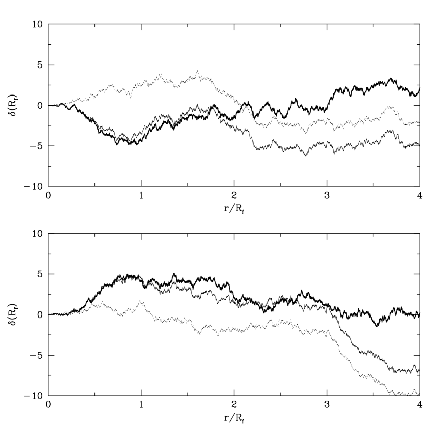
Figure 1: Examples of trajectories obtained by smoothing the linear density fluctuation field with a series of sharp $k$-space filters (with decreasing resolution scales $R_{f}=1/k_{f}$) at two points separated by the distance $r$. Here we consider $r=4\,{\rm Mpc}$ and a CDM power spectrum (with density parameter $\Omega=1$ and present Hubble constant $H_{\circ}=50\,{\rm km\,s^{-1}}\,{\rm Mpc}^{-1}$) linearly extrapolated to $\sigma_{8}=1$. The heavy continuous line represents the trajectory associated to a point ${\bf x}$ in Lagrangian space. The trajectory associated to the point ${\bf y}$ such that $|{\bf y}-{\bf x}|=r$ is plotted with a light continuous line. The dotted line is obtained by: i) considering the trajectory associated to ${\bf y}$, ii) artificially removing any correlation with the trajectory at ${\bf x}$ and iii) suitably rescaling the result. In practice, the dotted line represents a trajectory which is completely independent of the one associated to ${\bf x}$, but which has the same statistical one-point properties. This is what is generally used in building up merger trees of dark matter haloes. However, the actual trajectories associated to neighbouring points are strongly correlated when the smoothing length $R_{f}$ is comparable to the physical separation between the points $r$. The same trajectories tend to become less and less correlated as $R_{f}$ decreases. It is interesting to note that a memory of the strong correlation existing for $r/R_{f}\ll 1$ remains even when $r/R_{f}\gg 1$. In fact, when $R_{f}$ is small compared to $r$, the real trajectory associated to ${\bf y}$ can be accurately approximated by adding a constant value to the independent trajectory so that it matches the random walk at ${\bf x}$ when $R_{f}\raise-2.0pt\hbox{\hbox to0.0pt{\hbox{$\sim$}\hss}\raise 5.0pt\hbox{$>$}\ }\,r$. In other words, since the trajectories are continuous functions of $R_{f}$, the value assumed at $R_{f}\sim r$ (i.e. at the end of the strongly correlated regime) represents the initial condition for the random walk at small $R_{f}$ (i.e. in the independent regime). This derives from a sort of natural peak-background split: by evaluating the density fluctuation field in two points separated by $r$ one samples the same background value (obtained by summing up all the Fourier components corresponding to wavelenghts larger than $r$) but different high frequency modes.

In the latter approach, however, spatial correlations between different branches of the tree as well as correlations between different trees are completely ignored. The existence of this shortcoming has been also noticed by Rodrigues & Thomas (1996) in connection with the so-called ‘block model’ (Cole & Kaiser 1988; Cole 1991), which can be considered as a rudimentary form of merging tree, where haloes can only grow by doubling their mass. Yano, Nagashima & Gouda (1996) and Nagashima & Gouda (1997) analysed the possible changes induced by spatial correlations on the PS mass function.

The problem within the standard Monte Carlo approach is that each trajectory is treated as being independent of all the others. In a general Gaussian field, however, this situation is not realized and, for power-spectra of cosmological interest, the density fluctuations turn out to be strongly correlated on small scales. This statistical property can be clearly detected by looking at a pair of trajectories associated to two neighbouring points. In Fig. 1 we show two trajectories obtained by smoothing a correlated field with a sharp $k$-space filter. When the smoothing length is much larger than the separation between the points in which the trajectories are computed the density contrast assumes values that are practically coincident. On the other hand, for filtering radii much smaller than the lag that separates the points, the trajectories become indeed uncorrelated. The transition from the completely correlated situation to the totally uncorrelated one is continuous, i.e. the trajectories become less and less correlated as the smoothing length decreases. For comparison, in Fig. 1 we also show the same trajectories modified by artificially removing any correlation between them. It is clear that the joint distribution of first upcrossings at different points is heavily influenced by the correlations of the underlying density fluctuation field.

In this paper we will i) compute the joint two-point distribution of the first upcrossing events and use the solution to obtain an approximate analytical expression for the halo-halo correlation function, ii) numerically solve suitable sets of spatially correlated Langevin equations to directly compute the halo two-point function at different lags. In a forthcoming paper we will consider the effects of correlations on the merging histories of dark matter haloes.

The plan of the paper is as follows. In Section 2 we present a straightforward extension of the excursion set approach and review the standard application of this method which allows to determine the mean mass function of DM haloes. In Section 3 we study the Lagrangian clustering of haloes identified by our scheme and obtain the halo-halo correlation function both from an approximate analytic treatment and from a numerical integration of two spatially correlated Langevin equations. Section 4 contains a discussion of our results and hints at some applications of our algorithm to generate spatially correlated halo merger trees.

2 Excursion set approach

In this section we review the formulation of the excursion set approach, mostly following the treatment given by BCEK.

2.1 Langevin equation

Let us assume that the linear density fluctuations form a homogeneous and isotropic Gaussian random field $\delta({\bf x},z)$, with $\bf x$ the Lagrangian comoving position and $z$ the redshift. In linear theory one can factor out the redshift dependence as $D(z)\delta({\bf x})$, where $D(z)$ is the linear growth factor (e.g. Peebles 1980). With the normalization $D(z=0)=1$, $\delta({\bf x})$ becomes the mass density fluctuation linearly extrapolated to the present epoch.

The statistical properties of the Gaussian field $\delta({\bf x})$ are completely specified by the two-point function in Fourier space, which is related to the power-spectrum $P(k)$ by $\langle\tilde{\delta}({\bf k}_{1})\,\tilde{\delta}({\bf k}_{2})\rangle=(2\pi)^{3}\delta_{{}_{D}}({\bf k}_{1}+{\bf k}_{2})P(k_{1})$. The symbol $\delta_{{}_{D}}$ represents the Dirac delta function, and the brackets $\langle\cdot\rangle$ denote ensemble averaging. Our Fourier transform convention is $\tilde{\delta}({\bf k})=\int d{\bf x}\,\delta({\bf x})\,{\rm e}^{i{\bf k}\cdot{\bf x}}$.

We want now to study the statistical properties of the density fluctuation field at some resolution scale $R_{f}$. This is introduced by convolving $\delta({\bf x})$ by some filter function $W(|{\bf x}^{\prime}-{\bf x}|,R_{f})$,

$$\delta({\bf x},R_{f})=\int d{\bf x}^{\prime}\,W(|{\bf x}^{\prime}-{\bf x}|,R_{f})\,\delta({\bf x}^{\prime})=\frac{1}{(2\pi)^{3}}\int d{\bf k}\,\widetilde{W}(kR_{f})\,\tilde{\delta}({\bf k})\,{\rm e}^{-i{\bf k}\cdot{\bf x}}\;,$$ (1)

where $\widetilde{W}$ is the Fourier transform of the filter. At each point ${\bf x}$ the smoothed field represents the weighted average of $\delta({\bf x})$ over a spherical region of characteristic dimension $R_{f}$ centred in ${\bf x}$. The detailed properties of $\delta({\bf x},R_{f})$ clearly depend upon the specific choice of window function. The most commonly used smoothing kernels are the top-hat filter $W_{TH}(|{\bf x}|,R_{f})=3\,\Theta(R_{f}-|{\bf x}|)/4\pi R_{f}^{3}$, where $\Theta(x)$ is the Heaviside step function, and the Gaussian one $W_{G}(x,R_{f})=(2\pi R_{f}^{2})^{-3/2}\exp(-x^{2}/2R_{f}^{2})$. Recently, for convenience of analysis, top-hat filtering has been also applied in momentum space $\widetilde{W}_{SKS}(k,R_{f})=\Theta(k_{f}-k)$, where $k_{f}=1/R_{f}$ and $k_{f}=|{\bf k}_{f}|$. This kernel is generally called sharp $k$-space filter. While it is easy to associate a mass to real space top-hat filtering $M_{TH}(R_{f})=4\pi\rho_{b}R_{f}^{3}/3$, there is always a bit of arbitrariness in assigning a mass to the other window functions. The most common procedure is to multiply the average density by the volume enclosed by the filter, obtaining $M_{G}(R_{f})=(2\pi)^{3/2}\rho_{b}R_{f}^{3}$ and $M_{SKS}(R_{f})=6\pi^{2}\rho_{b}k_{f}^{-3}$ (Lacey & Cole 1993). An alternative procedure, originally introduced by Bardeen et al. (1986), corresponds to the choice $M_{SKS}(R_{f})=4\pi\rho_{b}R_{TH}^{3}/3$, where $R_{TH}$ is chosen by requiring $\sigma^{2}_{SKS}(R_{f})=\sigma^{2}_{TH}(R_{TH})$, and similarly for the Gaussian filter. In this way one obtains good agreement with numerical simulations of clustering growth (Lacey & Cole 1994).

In hierarchical bottom-up models of structure formation at each epoch mass fluctuations have typically undergone non-linear collapse up to some scale $R_{f}$, and the first objects that form are those of lower mass. Haloes of larger mass arise by the merging and accretion of subunits. The mass distribution deriving from this hierarchical halo formation process has been successfully modeled by Peacock & Heavens (1990), Cole (1991), BCEK and Lacey & Cole (1993). In order to mimic the accretion of matter all these models consider a full hierarchy of decreasing resolution scales $R_{f}$. The effect of varying $R_{f}$ can be obtained by differentiating eq. (1)

$${\partial\delta({\bf x},R_{f})\over\partial R_{f}}={1\over(2\pi)^{3}}\int d{\bf k}\,\tilde{\delta}({\bf k})\,{\partial\widetilde{W}(kR_{f})\over\partial R_{f}}\,{\rm e}^{-i{\bf k}\cdot{\bf x}}\equiv\eta({\bf x},R_{f})\;.$$ (2)

This has the form of a Langevin equation, which shows how an infinitesimal change of the resolution scale $R_{f}$ affects the value of the density fluctuation field $\delta({\bf x},R_{f})$ in the given position ${\bf x}$ through the action of the stochastic force $\eta({\bf x},R_{f})$. In the limit $R_{f}\to\infty$ one has $\delta({\bf x};R_{f})\to 0$, which can be adopted as initial condition for our first-order stochastic differential equation. Thus, by solving it, we can associate to each point ${\bf x}$ a trajectory $\delta({\bf x},R_{f})$ obtained by varying the resolution scale $R_{f}$. Notice that, since eq. (2) is linear, $\eta({\bf x},R_{f})$ is also a zero mean Gaussian random field, uniquely specified by its auto-correlation function

$$\langle\eta({\bf x}_{1},R_{f1})\,\eta({\bf x}_{2},R_{f2})\rangle={1\over 2\pi^{2}}\int_{0}^{\infty}dk_{1}\,k_{1}^{2}\,P(k_{1})\,{\partial\widetilde{W}(k_{1}R_{f1})\over\partial R_{f1}}\,{\partial\widetilde{W}(k_{1}R_{f2})\over\partial R_{f2}}\,j_{0}(k_{1}r)\;,$$ (3)

where $r=|{\bf x}_{1}-{\bf x}_{2}|$ and $j_{0}(x)$ is the zeroth order spherical Bessel function. Trajectories associated to different neighbouring points will be statistically influenced by the correlation properties of the force $\eta({\bf x},R_{f})$, i.e. of the underlying Gaussian field $\delta({\bf x})$. On the other hand the coherence of each trajectory along the $R_{f}$ direction depends exclusively on the analytic form of the filter function and vanishes for the sharp $k$-space window (BCEK). With such a filter, by decreasing the smoothing length one adds up a new set of Fourier modes of the unsmoothed distribution to $\delta({\bf x},R_{f})$. For a Gaussian field this is completely independent of the previous increments, and each trajectory $\delta({\bf x},R_{f})$ becomes a Brownian random walk.

In the case of sharp $k$-space filtering the notation greatly simplifies if we use as time variable the variance of the filtered density field, $\Lambda\equiv\sigma^{2}(k_{f})=\langle\delta(k_{f})^{2}\rangle=(2\pi^{2})^{-1}\int_{0}^{k_{f}}dk\,k^{2}\,P(k)$. In such a case the stochastic process reduces to a Wiener one, namely

$$\frac{\partial\delta({\bf x},\Lambda)}{\partial\Lambda}=\zeta({\bf x},\Lambda)\;,$$ (4)

with $\langle\zeta({\bf x},\Lambda)\rangle=0$ and

$$\langle\zeta({\bf x},\Lambda_{1})\,\zeta({\bf x},\Lambda_{2})\rangle=\delta_{{}_{D}}(\Lambda_{1}-\Lambda_{2})$$ (5)

[see eq. (17) for the spatial correlation]. In the following we will adopt $\Lambda$ as time variable, unless explicitly stated. The solution of the Langevin equation (4) in an arbitrary point of space (the position ${\bf x}$ is here understood), with the initial condition $\delta(\Lambda=0)=0$, is simply $\delta(\Lambda)=\int_{0}^{\Lambda}d\Lambda^{\prime}\zeta(\Lambda^{\prime})$. By ensemble averaging this expression one obtains $\langle\delta(\Lambda)\rangle=0$ and $\langle\delta(\Lambda_{1})\delta(\Lambda_{2})\rangle={\rm min}(\Lambda_{1},\Lambda_{2})$, which uniquely determine the Gaussian distribution of $\delta(\Lambda)$. More details can be found in Porciani et al. (1996).

2.2 Press-Schechter mass function

Press & Schechter (1974) proposed a simple model to compute the comoving number density of collapsed haloes directly from the statistical properties of the linear Gaussian density field (see also Doroshkevich 1967). According to the PS theory a patch of fluid is part of a collapsed region of scale larger than $M(R_{f})$ if the value of the smoothed linear density contrast on the same scale exceeds a threshold $t_{f}$. The idea is to use a global threshold in order to mimic non-linear dynamical effects ending up to halo collapse and virialization. An exact value for $t_{f}$ can be obtained by describing the evolution of density perturbations according to the spherical top-hat model. In this case a fluctuation of amplitude $\delta$ will collapse at a redshift $z_{f}$ such that $\delta({\bf x})=t_{f}\equiv\delta_{c}/D(z_{f})$. In the Einstein de Sitter universe and during the matter dominated era the critical value $\delta_{c}$ does not depend on any cosmological parameter and is given by $\delta_{c}=3(12\pi)^{2/3}/20\simeq 1.686$, whereas, for general cosmologies, it shows a weak dependence on the value of the density parameter, the cosmological constant, the Hubble constant, thus on redshift (e.g. Lacey & Cole 1993).

The PS formula for the mass function has been thoroughly compared with the outcomes of N-body simulations, finding general good agreement (e.g. Efstathiou et al. 1988; Gelb & Bertschinger 1994; Lacey & Cole 1994). As mentioned in the Introduction, the model is intrinsically flawed by the cloud-in-cloud problem, namely the fact that a fluctuation on a given scale can contain substructures of smaller scales and the same fluid elements can be assigned, according to the PS collapse criterion, to haloes of different mass. Moreover, in a hierarchical scenario, one expects to find all the mass collapsed in objects of some scale, while the PS model can account only for half of it: this problem is intimately related to the fact that in a Gaussian field only half volume is overdense. Press and Schechter faced the problem by simply multiplying their result by a fudge factor of 2. In this section we review how the Langevin equations introduced above can be used to extend the PS theory in such a way to solve both problems. In the next sections we will use the same approach to compute the halo-halo correlation function.

The solution of the cloud-in-cloud problem has been given by Peacock & Heavens (1990), Cole (1991) and BCEK. Their approach consists in considering at any given point the trajectory $\delta(R_{f})$ as a function of the filtering radius, and then determining the largest $R_{f}$ at which $\delta(R_{f})$ upcrosses the threshold $t_{f}(z_{f})$ corresponding to the formation redshift $z_{f}$. This determines the largest mass collapsed at that point, all sub-structures having been erased. So, the computation of the mass function is equivalent to calculating the fraction of trajectories that first upcross the threshold $t_{f}$ as the scale $M$ decreases. The solution of the problem is enormously simplified for Brownian trajectories, that is for sharp $k$-space filtered density fields. In such a case one only has to solve the Fokker-Planck equation for the probability density ${\cal W}(\delta,\Lambda)\,d\delta$ that the stochastic process at $\Lambda$ assumes a value in the interval $\delta,\delta+d\delta$,

$$\frac{\partial{\cal W}(\delta,\Lambda)}{\partial\Lambda}=\frac{1}{2}\,\frac{\partial^{2}{\cal W}(\delta,\Lambda)}{\partial\delta^{2}}\;,$$ (6)

with the absorbing boundary condition ${\cal W}(t_{f},\Lambda)=0$ and initial condition ${\cal W}(\delta,0)=\delta_{D}(\delta)$. The solution is well known (Chandrasekhar 1943)

$${\cal W}(\delta,\Lambda;t_{f})\,d\delta={1\over\sqrt{2\pi\Lambda}}\left[\exp\left(-{\delta^{2}\over 2\Lambda}\right)-\exp\left(-{(\delta-2t_{f})^{2}\over 2\Lambda}\right)\right]\,d\delta\;.$$ (7)

Defining $\,S(\Lambda,t_{f})=\int_{-\infty}^{t_{f}}\!d\delta\,{\cal W}(\delta,\Lambda,t_{f})\,$ as survival probability of the trajectories, one obtains the density probability distribution of first-crossing variances by differentiation

$${\cal P}_{1}(\Lambda)=-{\partial S(\Lambda,t_{f})\over\partial\Lambda}=-{\partial\over\partial\Lambda}\int_{-\infty}^{t_{f}}\!d\delta\,{\cal W}(\delta,\Lambda;t_{f})=\left[-{1\over 2}{\partial{\cal W}(\delta,\Lambda,t_{f})\over\partial\delta}\right]_{-\infty}^{t_{f}}={t_{f}\over\sqrt{2\pi\Lambda^{3}}}\exp\left(-{t_{f}^{2}\over 2\Lambda}\right)\;.$$ (8)

The function ${\cal P}_{1}(\Lambda)\,d\Lambda$ yields the probability that a realization of the random walk is absorbed by the barrier in the interval $(\Lambda,\Lambda+d\Lambda)$ or, by the ergodic theorem, the probability that a fluid element belongs to a structure with mass in the range [$M(\Lambda+d\Lambda),M(\Lambda)$]. Finally, the comoving number density of haloes with mass in the interval $[M,M+dM]$ collapsed at redshift $z_{f}$ is

$$n(M,z_{f})\,dM={\rho_{b}\over M}\,{\cal P}_{1}(\Lambda)\,\left|{d\Lambda\over dM}\right|\,dM\;.$$ (9)

Inserting the expression of ${\cal P}_{1}(\Lambda)$ of eq. (8) in the latter equation one obtains the well-known PS expression for the mass function

$$n(M,z_{f})\,dM={\rho_{b}\,t_{f}(z_{f})\over\sqrt{2\pi}}\,{1\over M^{2}\sqrt{\Lambda(M)}}\,\left|{d\ln\Lambda\over d\ln M}\right|\;\exp\left(-{t_{f}(z_{f})^{2}\over 2\,\Lambda(M)}\right)\,dM\;.$$ (10)

The original fudge factor of 2 of the PS approach is now naturally justified. A generalization of this formalism to simple cases of non-Gaussian initial conditions has been given by Porciani et al. (1996).

Previous investigations (e.g. Peacock & Heavens 1990; BCEK) have shown that only for sharp $k$-space filtering it is possible to write an analytic formula for the mass function obtained from the excursion set approach. Numerical solutions of the cloud-in-cloud problem with physically more acceptable smoothing kernels like Gaussian and top-hat result in mass functions that are a factor of two lower in the high-mass tail and have different small-mass slopes compared with the PS formula. The standard interpretation of this result is that the excursion set method is not reliable for $M\ll M_{\ast}$, where $M_{\ast}$, defined by $\Lambda(M_{\ast})=t_{f}^{2}$, is the typical mass collapsing at $z_{f}$.

3 Lagrangian clustering

In this section we show how the excursion set approach can be extended to derive the clustering properties of dark matter haloes. Specifically, we study the evolution of a set of density fluctuation processes at different spatial locations, as the smoothing scale progressively shrinks. The trajectories turn out to be intimately correlated and the joint distribution of the first upcrossing filtering radii is used to extract the Lagrangian halo-halo correlation function.

3.1 Two-point correlation function from joint upcrossing distribution

Let us select two points in Lagrangian space ${\bf x}_{1}$ e ${\bf x}_{2}={\bf x}_{1}+{\bf r}$. We want to study the evolution of the stochastic processes $\delta_{1}(\Lambda)=\delta({\bf x}_{1},\Lambda)$ and $\delta_{2}(\Lambda)=\delta({\bf x}_{2},\Lambda)$ as $\Lambda$ varies. In particular, let us suppose that we know the joint probability distribution ${\cal P}_{2}(\Lambda_{1},\Lambda_{2};{\bf x}_{1},{\bf r})$ of those pairs of variances $(\Lambda_{1},\Lambda_{2})$ that correspond to the first upcrossing scales of the threshold $t_{f}$ by the two processes $\delta_{1}(\Lambda)$ and $\delta_{2}(\Lambda)$. Because of the underlying homogeneity and isotropy, the probability density ${\cal P}_{2}$ cannot depend on the vector ${\bf x}_{1}$ and on the orientation of ${\bf r}$, i.e. ${\cal P}_{2}(\Lambda_{1},\Lambda_{2};{\bf x}_{1},{\bf r})={\cal P}_{2}(\Lambda_{1},\Lambda_{2};r)$. Moreover, by the ergodic theorem one can identify ${\cal P}_{2}(\Lambda_{1},\Lambda_{2};r)$ with the probability distribution of the pairs $(\Lambda_{1},\Lambda_{2})$, obtained by randomly selecting points spatially separated by the distance $r$, within a given realization of the density field. Finally, following the arguments given in the previous section, we can interpret ${\cal P}_{2}(\Lambda_{1},\Lambda_{2};r)\,d\Lambda_{1}d\Lambda_{2}$ as the probability of finding two points separated by $r$ within two haloes with mass in the intervals $(M_{1}-dM_{1},M_{1})$ and $(M_{2}-dM_{2},M_{2})$, as fixed by the corresponding variance ranges $(\Lambda_{1},\Lambda_{1}+d\Lambda_{1})$ and $(\Lambda_{2},\Lambda_{2}+d\Lambda_{2})$. As we will discuss in detail in the next sections, the probability density ${\cal P}_{2}(\Lambda_{1},\Lambda_{2};r)$ can be obtained by integrating the system of correlated Langevin equations that describe the evolution of the processes $\delta_{1}(\Lambda)$ and $\delta_{2}(\Lambda)$.

In order to compute the halo-halo correlation function we adopt the following procedure. A class of objects is selected by the mass interval corresponding to the $\Lambda$-range $I\equiv[\Lambda_{\rm min},\Lambda_{\rm max}]$. The probability of determining two points separated by $r$ contained within collapsed objects of class $I$ is

$${\cal P}_{II}(r)=\int_{I}\int_{I}d\Lambda_{1}\,d\Lambda_{2}\,{\cal P}_{2}(\Lambda_{1},\Lambda_{2};r)\;.$$ (11)

Similarly, the probability of finding a point contained in an object of type $I$ is ${\cal P}_{I}=\int_{I}d\Lambda\,{\cal P}_{1}(\Lambda)$. From the definition of correlation function we then obtain

$$\xi_{II}^{pts}(r)={{\cal P}_{II}\over{\cal P}_{I}^{2}}-1={\int_{I}\int_{I}d\Lambda_{1}\,d\Lambda_{2}\,{\cal P}_{2}(\Lambda_{1},\Lambda_{2};r)\over\left[\int_{I}d\Lambda\,{\cal P}_{1}(\Lambda)\right]^{2}}-1\;.$$ (12)

In a similar fashion, considering disjoint classes $I_{1}$ and $I_{2}$,

$$\xi_{I_{1}I_{2}}^{pts}(r)={\int_{I_{1}}\int_{I_{2}}d\Lambda_{1}\,d\Lambda_{2}\,{\cal P}_{2}(\Lambda_{1},\Lambda_{2};r)\over\int_{I_{1}}d\Lambda\,{\cal P}_{1}(\Lambda)\,\int_{I_{2}}d\Lambda\,{\cal P}_{1}(\Lambda)}-1\;.$$ (13)

We stress that the quantities $\xi_{II}^{pts}(r)$ and $\xi_{I_{1}I_{2}}^{pts}(r)$ are the Lagrangian correlations of the mass elements contained in the collapsed haloes. This quantity has been recently used by Bagla (1997) to study the evolution of galaxy clustering. However, we are ultimately concerned with the calculation of the halo correlations $\xi_{II}^{hh}(r)$, so we have to properly weigh the statistical contribution for each extended halo. The problem shows particularly simple if we adopt the PS theory. Indeed, in this case, the sets of points where the first upcrossings occur at the same $\Lambda$ are point-like disconnected regions (see Bond & Myers 1996 for a different approach). Only in a statistical sense they originate collapsed haloes, each contributing by $1/V(\Lambda)$, where $V(\Lambda)\equiv M/\rho_{b}$ is the typical Lagrangian volume of an object of mass $M$ associated to the variance $\Lambda$. Therefore, adopting the same procedure used to calculate the mass function, the mean number density of collapsed objects of scale $\Lambda$ becomes $n(\Lambda)={\cal P}_{1}(\Lambda)/V(\Lambda)$. Similarly, for the distribution of pairs at distance $r$, we define

$$n_{2}(\Lambda_{1},\Lambda_{2};r)={{\cal P}_{2}(\Lambda_{1},\Lambda_{2};r)\over V(\Lambda_{1})V(\Lambda_{2})}\;.$$ (14)

The idea is, once again, to allow for the finite size of the haloes. The halo-halo correlations become, respectively,

$$\xi_{II}^{hh}(r)={n_{II}\over n_{I}^{2}}-1\equiv{\int_{I}\int_{I}d\Lambda_{1}d\Lambda_{2}\,n_{2}(\Lambda_{1},\Lambda_{2};r)\over\left[\int_{I}d\Lambda\,n(\Lambda)\right]^{2}}-1\;,$$ (15)

and

$$\xi_{I_{1}I_{2}}^{hh}(r)={\int_{I_{1}}\int_{I_{2}}d\Lambda_{1}d\Lambda_{2}\,n_{2}(\Lambda_{1},\Lambda_{2},r)\over\int_{I_{1}}d\Lambda\,n(\Lambda)\int_{I_{2}}d\Lambda\,n(\Lambda)}-1\;.$$ (16)

3.2 Correlated Langevin equations: sharp k-space filtering

In Section 3.1 we showed that, in order to obtain the halo correlation function, it is crucial to know the joint distribution ${\cal P}_{2}(\Lambda_{1},\Lambda_{2};r)$. This quantity can be obtained by solving the system of equations governing the evolution of the pair of correlated processes $\delta_{1}(\Lambda)$ and $\delta_{2}(\Lambda)$:

$$\left\{\begin{array}[]{l}{\displaystyle{\partial\delta_{1}(\Lambda)\over\partial\Lambda}=\zeta_{1}(\Lambda)\;,\;\;\;\;\;\;\;\;\;\;\;\;\;\;\;\;\;\delta_{1}(0)=0}\;,\\ \\ {\displaystyle{\partial\delta_{2}(\Lambda)\over\partial\Lambda}=\zeta_{2}(\Lambda)\;,\;\;\;\;\;\;\;\;\;\;\;\;\;\;\;\;\;\delta_{2}(0)=0}\;,\\ \\ \langle\zeta_{1}(\Lambda)\rangle=\langle\zeta_{2}(\Lambda)\rangle=0\;,\;\;\;\;\;\;\;\;\zeta_{1}\;\,{\rm and}\;\,\zeta_{2}\;\,{\rm Gaussian\;\;\,processes}\;,\\ \\ {\displaystyle\langle\zeta_{1}(\Lambda)\,\zeta_{1}(\Lambda^{\prime})\rangle=\langle\zeta_{2}(\Lambda)\,\zeta_{2}(\Lambda^{\prime})\rangle=\delta_{D}(\Lambda-\Lambda^{\prime})}\;,\\ \\ {\displaystyle\langle\zeta_{1}(\Lambda)\,\zeta_{2}(\Lambda^{\prime})\rangle=\frac{\partial\xi(r;\Lambda)}{\partial\Lambda}\,\delta_{D}(\Lambda-\Lambda^{\prime})}\;.\end{array}\right.$$ (17)

The latter equation, obtained by introducing sharp $k$-space filtering in equation (3), completes the definition of the stochastic field $\zeta({\bf x},\Lambda)$ given in equations (4) and (5). Here $\xi(r;\Lambda)$ is the linear two-point correlation function for the mass density fluctuations smoothed on the scale $R_{f}\equiv 1/k_{f}$ associated to the variance $\Lambda$

$$\xi(r;\Lambda)\equiv{1\over 2\pi^{2}}\int_{0}^{k_{f}\!(\Lambda)}dk\,k^{2}\,P(k)\;j_{0}(kr)\;$$ (18)

and one has

$$\frac{\partial\xi(r;\Lambda)}{\partial\Lambda}=j_{0}[k_{f}(\Lambda)\,r]\;.$$ (19)

By integrating the above differential equations and averaging over the ensemble one obtains the unconstrained probability distribution

$${\cal W}_{r}(\delta_{1},\delta_{2};\Lambda)={1\over 2\pi\sqrt{\Lambda^{2}-\xi(r;\Lambda)^{2}}}\,\exp{\left[-{\Lambda(\delta_{1}^{2}+\delta_{2}^{2})-2\,\xi(r;\Lambda)\,\delta_{1}\delta_{2}\over 2\left[\Lambda^{2}-\xi(r;\Lambda)^{2}\right]}\right]}\;.$$ (20)

This function solves the two-dimensional Fokker-Planck equation associated to the Langevin equation (17), namely

$${\partial{\cal W}_{r}(\delta_{1},\delta_{2};\Lambda)\over\partial\Lambda}=\frac{1}{2}\left[\frac{\partial^{2}}{\partial\delta_{1}^{2}}+\frac{\partial^{2}}{\partial\delta_{2}^{2}}\,+\,2\,\frac{\partial\xi(r;\Lambda)}{\partial\Lambda}\,\frac{\partial^{2}}{\partial\delta_{1}\partial\delta_{2}}\right]\,{\cal W}_{r}(\delta_{1},\delta_{2};\Lambda)\;,$$ (21)

with initial condition ${\cal W}_{r}(\delta_{1},\delta_{2},\Lambda=0)=\delta_{{}_{D}}(\delta_{1})\,\delta_{{}_{D}}(\delta_{2})$. The problem of finding the distribution of the first upcrossings of the threshold $t_{f}$ by the binary process $\{\delta_{1},\delta_{2}\}$ reduces to that of imposing proper boundary conditions to the equation (21). As done for the one-dimensional Fokker-Planck equation, we adopt the absorbing barrier approach. However, in the two-dimensional case we are considering, the distribution ${\cal P}_{2}(\Lambda_{1},\Lambda_{2};r)$ cannot be eventually obtained from ${\cal W}_{r}(\delta_{1},\delta_{2};\Lambda)$ simply by differentiation. This is because the whole binary system automatically disappears as soon as when one ‘Brownian particle’ is first absorbed. Nonetheless, the joint distribution ${\cal P}_{2}(\Lambda_{1},\Lambda_{2};r)$ can be in principle calculated by a two-step procedure as follows.

Assuming the same initial condition, one solves the Fokker-Planck equation with absorbing barriers at $\delta_{1}=t_{f}$ and $\delta_{2}=t_{f}$, thus finding the survival probability density for the pairs which have never crossed the thresholds. Having found this quantity one can compute the probability current through each point,

$${\bf J}(\delta_{1},\delta_{2};\Lambda)=-\frac{1}{2}\left(\frac{\partial{\cal W}_{r}}{\partial\delta_{1}}+\frac{\partial\xi(r;\Lambda)}{\partial\Lambda}\,\frac{\partial{\cal W}_{r}}{\partial\delta_{2}}\,,\;\;\;\frac{\partial\xi(r;\Lambda)}{\partial\Lambda}\,\frac{\partial{\cal W}_{r}}{\partial\delta_{1}}+\frac{\partial{\cal W}_{r}}{\partial\delta_{2}}\right)\;.$$ (22)

On a boundary wall, e.g. $\delta_{1}=t_{f}$, where ${\cal W}_{r}(t_{f},\delta_{2};\Lambda)=0$ (implying $\partial{\cal W}_{r}/\partial\delta_{2}=0$), this reduces to

$${\bf J}(t_{f},\delta_{2};\Lambda)=-\frac{1}{2}\left(\left.\frac{\partial{\cal W}_{r}}{\partial\delta_{1}}\right|_{t_{f}}\,,\;\;\;\frac{\partial\xi(r;\Lambda)}{\partial\Lambda}\,\left.\frac{\partial{\cal W}_{r}}{\partial\delta_{1}}\right|_{t_{f}}\right)\;.$$ (23)

The flux through any point of the barrier $\delta_{1}=t_{f}$ is then given by the scalar product ${\bf J}\cdot{\bf n}$, where ${\bf n}\equiv(1,0)$ is the unit vector perpendicular to the absorbing wall,

$${\cal F}_{r}(t_{f},\delta_{2};\Lambda)=-\frac{1}{2}\,\left.\frac{\partial{\cal W}_{r}}{\partial\delta_{1}}\right|_{t_{f}}\;.$$ (24)

The quantity ${\cal F}_{r}(t_{f},\delta_{2};\Lambda)\,d\delta_{2}$ represents the probability that the pair of processes ($\delta_{1}$,$\delta_{2}$) leave the permitted region passing through the ‘gate’ $[(t_{f},\delta_{2}),(t_{f},\delta_{2}+d\delta_{2})]$ at the time $\Lambda$. This flux contains all the information we need for the computation of ${\cal P}_{2}(\Lambda_{1},\Lambda_{2};r)$. In fact, once $\delta_{1}$ has crossed the barrier at $\Lambda_{1}$, for $\Lambda>\Lambda_{1}$ we are interested in studying only the evolution of the surviving process $\delta_{2}$ up to its first upcrossing through the boundary $\delta_{2}=t_{f}$. Therefore, since we are considering Brownian trajectories, free of correlations along the $\Lambda$ axis, for $\Lambda>\Lambda_{1}$ the evolution of $\delta_{2}$ is simply governed by its own Langevin equation, and its probability distribution can be calculated from the one-dimensional Fokker-Planck equation (6), with absorbing boundary $\delta_{2}=t_{f}$, but with initial condition (at $\Lambda=\Lambda_{1}$) $\delta_{2\ast}\equiv\delta_{2}(\Lambda_{1}|\delta_{1}=t_{f})$. Thus, by simply modifying eq. (8), we find that the distribution of the variances $\Lambda_{2}$ associated to first upcrossing events of the threshold by the process $\delta_{2}$, given that $\delta_{1}$ upcrossed the critical level at $\Lambda_{1}$, is:

$${\cal P}_{1}(\Lambda_{2}-\Lambda_{1},t_{f}-\delta_{2\ast})={(t_{f}-\delta_{2\ast})\over\sqrt{2\pi}~{}(\Lambda_{2}-\Lambda_{1})^{3/2}}\exp\left[-{(t_{f}-\delta_{2\ast})^{2}\over 2(\Lambda_{2}-\Lambda_{1})}\right]\;.$$ (25)

The joint distribution ${\cal P}_{2}(\Lambda_{1},\Lambda_{2};r)$ is eventually obtained by a convolution

$${\cal P}_{2}(\Lambda_{1},\Lambda_{2};r)=\int_{-\infty}^{t_{f}}d\delta_{2}\,{\cal F}_{r}(t_{f},\delta_{2};\Lambda_{1})\,{\cal P}_{1}(\Lambda_{2}-\Lambda_{1},t_{f}-\delta_{2})+\int_{-\infty}^{t_{f}}d\delta_{1}\,{\cal F}_{r}(\delta_{1},t_{f};\Lambda_{2})\,{\cal P}_{1}(\Lambda_{1}-\Lambda_{2},t_{f}-\delta_{1})\;,$$ (26)

where the first and second integrals on the r.h.s. represent, respectively, the contributions of those pairs for which $\Lambda_{2}\geq\Lambda_{1}$ and $\Lambda_{2}<\Lambda_{1}$.

However, this formal expression is useless unless we solve for the probability density ${\cal W}_{r}$. There are two cases in which the calculation of ${\cal W}_{r}$ is trivial: one for $r\to\infty$ and the other for $r\to 0$. The general case of finite non-zero lag $r$ is far more complex, as we will discuss.

3.2.1 Perfectly uncorrelated processes

At infinite lag ($r\to\infty$) the two processes become independent and the solution of the Fokker-Planck equation is

$${\cal W}_{\infty}(\delta_{1},\delta_{2};\Lambda)={\cal W}(\delta_{1},\Lambda;t_{f})\,{\cal W}(\delta_{2},\Lambda;t_{f})\;,$$ (27)

where ${\cal W}(\delta,\Lambda;t_{f})$ denotes the probability distribution for a one-dimensional process with absorbing boundary at $t_{f}$ given in eq. (7). This solution consists of a linear superposition of four unconstrained independent density distributions deriving from different initial conditions. In practice one has to consider the ‘real’ initial distribution $\delta_{{}_{D}}(0,0)$, an image source $\delta_{{}_{D}}(t_{f},t_{f})$ and two image sinks $\delta_{{}_{D}}(t_{f},0)$ and $\delta_{{}_{D}}(0,t_{f})$, that is to say

$${\cal W}_{\infty}(\delta_{1},\delta_{2};\Lambda)={\cal G}_{\infty}(\delta_{1},\delta_{2};\Lambda)-{\cal G}_{\infty}(\delta_{1}-2t_{f},\delta_{2};\Lambda)-{\cal G}_{\infty}(\delta_{1},\delta_{2}-2t_{f};\Lambda)+{\cal G}_{\infty}(\delta_{1}-2t_{f},\delta_{2}-2t_{f};\Lambda)\;,$$ (28)

where ${\cal G}(\delta_{1},\delta_{2};\Lambda)\equiv[2\pi\Lambda]^{-1}\exp[-(\delta_{1}^{2}+\delta_{2}^{2})/2\Lambda]$ is the solution of the two-dimensional Fokker-Planck equation with natural boundary conditions: $\lim_{\delta_{i}\to\infty}{\cal G}(\delta_{1},\delta_{2};\Lambda)=0,i=1,2$. Obviously, using eq. (26) we obtain

$${\cal P}_{2}(\Lambda_{1},\Lambda_{2};r\to\infty)={\cal P}_{1}(\Lambda_{1},t_{f}){\cal P}_{1}(\Lambda_{2},t_{f})\;,$$ (29)

that, inserted in equations (12) and (13) or in equations (15) and (16), gives, as expected for infinite lag, $\xi^{pts}=\xi^{hh}=0$.

3.2.2 Perfectly correlated processes

When $r\to 0$ the two processes become more and more correlated so that, in the limit, we end up with a one-dimensional problem. In this case the solution of the Fokker-Planck equation is

$${\cal W}_{0}(\delta_{1},\delta_{2};\Lambda)={\cal W}(\delta_{1}+\delta_{2},4\Lambda;t_{f})\,\delta_{{}_{D}}(\delta_{1}-\delta_{2})\;,$$ (30)

where ${\cal W}(\delta,\Lambda;t_{f})$ denotes the probability distribution given in eq. (7). Expanding this expression as a superposition of Green’s functions, by using the method of image sources, we obtain

$${\cal W}_{0}(\delta_{1},\delta_{2};\Lambda)={\cal G}_{0}(\delta_{1},\delta_{2};\Lambda)-{\cal G}_{0}(\delta_{1}-2t_{f},\delta_{2}-2t_{f};\Lambda)\;,$$ (31)

where ${\cal G}_{0}(x,y;\Lambda)\equiv{\cal W}(x,\Lambda;t_{f})\delta_{{}_{D}}(x-y)$. In this case, for the joint distribution of first upcrossing variances, we find

$${\cal P}_{2}(\Lambda_{1},\Lambda_{2};r\to 0)={\cal P}_{1}(\Lambda_{1},t_{f})\,\delta_{{}_{D}}(\Lambda_{1}-\Lambda_{2})\;.$$ (32)

Consequently, we obtain $\xi^{pts}_{II}\to[1/\int_{I}\,d\Lambda\,{\cal P}(\Lambda)]-1$ and $\xi^{hh}_{II}\to\{\int_{I}\,d\Lambda\,P(\Lambda)/V(\Lambda)^{2}/[\int_{I}\,d\Lambda\,P(\Lambda)/V(\Lambda)]^{2}\}-1$. Similarly, $\xi^{pts}_{I_{1}I_{2}}\to 0$ and $\xi^{hh}_{I_{1}I_{2}}=0$.

3.2.3 Approximate general solution

In the limiting cases just discussed we were able to account for the boundary conditions by writing the solution in terms of a superposition of image-distributions, each one solving the Fokker-Planck equation. Regrettably, the position and the sign of the image sources of probability come out dependent on the correlation between the processes (i.e. on $r$). This fact suggests that we cannot write a general analytical solution by simply applying the image method. However, we will build here a simple function that satisfies the absorbing boundary conditions being also an accurate approximation for the solution of the correlated diffusion equation. In the next section we will test the accuracy of this solution against the numerical one.

It is evident that, for small separation $r\ll R_{f}$ (we remind the reader that we change the smoothing radius $R_{f}$ at fixed separation $r$), the perfectly correlated solution will represent a very good approximation to the true one. This can be easily deduced by the following argument. The two Gaussian stochastic processes $\Sigma(\Lambda)=\delta_{1}(\Lambda)+\delta_{2}(\Lambda)$ and $\Delta(\Lambda)=\delta_{1}(\Lambda)-\delta_{2}(\Lambda)$ are statistically independent, i.e. $\langle\Sigma(\Lambda)\Delta(\Lambda)\rangle=0$. The variances of their unconstrained probability distributions are, respectively, $\sigma^{2}_{\Sigma}=2\,[\Lambda+\xi(r;\Lambda)]$ and $\sigma^{2}_{\Delta}=2\,[\Lambda-\xi(r;\Lambda)]$. Therefore, for $r\ll R_{f}$ [i.e. for $\Lambda\ll\sigma^{2}(r)$, where $\sigma^{2}(r)$ denotes the variance of the mass density fluctuations smoothed on the scale $r$] where $\xi(r;\Lambda)\simeq\Lambda$, we have $\sigma^{2}_{\Delta}\simeq 0$ and the probability distribution of the variable $\Delta$ is practically a Dirac delta function centred on the zero value. This corresponds to the perfectly correlated situation. However, this regime is not interesting for computing the halo correlation function since the condition $r\ll R_{f}$ implies that the points in which we follow the trajectories that upcross the threshold are involved in the collapse of the same halo.

On the other hand, for $r\gg R_{f}$ (i.e. for $\Lambda\gg\sigma^{2}(r)$), we can replace in eq. (21) $\xi(r;\Lambda)$ with the unsmoothed linear mass-correlation $\xi_{m}(r)$. Therefore, eq. (21) simply becomes the uncorrelated two-dimensional diffusion equation that can be easily solved using the image method. Our ansatz for the full ${\cal W}_{r}(\delta_{1},\delta_{2};\Lambda)$ is then obtained by keeping the analytic form of the solution just obtained for $r\gg R_{f}$ but inserting in it the correlation function $\xi(r;\Lambda)$ to replace its large lag limit $\xi_{m}(r)$. Therefore, we have

$${\cal W}_{r}(\delta_{1},\delta_{2};\Lambda)={\cal G}_{r}^{+}(\delta_{1},\delta_{2};\Lambda)-{\cal G}_{r}^{-}(\delta_{1}-2t_{f},\delta_{2};\Lambda)-{\cal G}_{r}^{-}(\delta_{1},\delta_{2}-2t_{f};\Lambda)+{\cal G}_{r}^{+}(\delta_{1}-2t_{f},\delta_{2}-2t_{f};\Lambda)\;,$$ (33)

where

$${\cal G}_{r}^{\pm}={1\over 2\pi\sqrt{\Lambda^{2}-\xi(r;\Lambda)^{2}}}\,\exp{\left[-{\Lambda(\delta_{1}^{2}+\delta_{2}^{2})-2\,[\pm\xi(r;\Lambda)]\,\delta_{1}\delta_{2}\over 2\left[\Lambda^{2}-\xi(r)^{2}\right]}\right]}\;.$$ (34)

By using the symbol ${\cal G}_{r}^{\pm}$ we want to emphasize the correlation properties of the adopted Green’s function: ${\cal G}_{r}^{+}$ is a correct solution of the diffusion equation, while ${\cal G}_{r}^{-}$ does not solve it. However, to satisfy the boundary conditions, we need to insert it twice in the solution. The probability distribution given in eq. (33) will be a valid approximation to the proper one provided the term

$$\frac{\partial\xi(r;\Lambda)}{\partial\Lambda}\frac{\partial^{2}}{\partial\delta_{1}\partial\delta_{2}}\left[{\cal G}_{r}^{-}(\delta_{1}-2t_{f},\delta_{2};\Lambda)+{\cal G}_{r}^{-}(\delta_{1},\delta_{2}-2t_{f};\Lambda)\right]$$ (35)

can be neglected compared to the $\Lambda$-derivative of the expression in eq. (33). A three-dimensional representation of this approximate solution and of its contour levels is given in Fig. 2. Inserting eq. (33) into equations (24) and (26) we obtain

$${\cal P}_{2}(\Lambda_{1},\Lambda_{2};r) = \frac{t_{f}^{2}\Lambda_{1}\Lambda_{2}+\left[\Lambda_{1}\Lambda_{2}-t_{f}^{2}(\Lambda_{1}+\Lambda_{2})\right]\xi(r;\Lambda_{\rm m})+t_{f}^{2}\,\xi(r;\Lambda_{\rm m})^{2}-\xi(r;\Lambda_{\rm m})^{3}}{2\pi\left[\Lambda_{1}\Lambda_{2}-\xi(r;\Lambda_{\rm m})^{2}\right]^{5/2}}\times$$ (36)

$$\times \exp{\left[-\frac{t_{f}^{2}}{2}\frac{\Lambda_{1}+\Lambda_{2}-2\,\xi(r;\Lambda_{\rm m})}{\Lambda_{1}\Lambda_{2}-\xi(r;\Lambda_{\rm m})^{2}}\right]}\;,$$

where $\Lambda_{\rm m}={\rm min}(\Lambda_{1},\Lambda_{2})$.

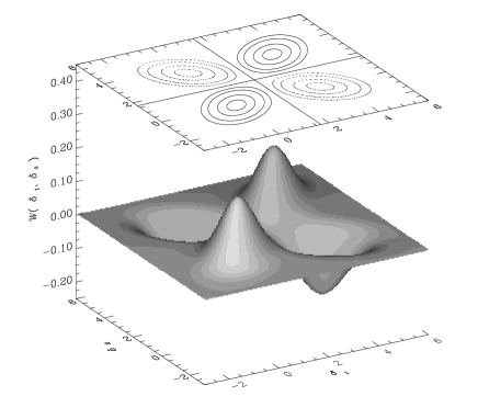
Figure 2: The approximate solution of the Fokker-Planck equation given in eq. (33) is plotted in the left panel (here $\Lambda=1$ and $\xi=0.4$). The probability density in the physical region is blown up in the right panel. In the contour plots the continuous lines correspond to the levels 0, 0.025, 0.05, 0.1, 0.15 (starting from outside), while the dotted lines refer to the same values multiplied by $-1$. The figure clearly shows that the proposed solution satisfies the absorbing boundary conditions for $\delta_{1}=t_{f}$ and $\delta_{2}=t_{f}$ (here $t_{f}=1.686$). Moreover, the orientation of the iso-probability curves in the allowed region (these are practically ellipses with their major axes lying on the line $\delta_{1}=\delta_{2}$) indicates that the approximate ${\cal W}(\delta_{1},\delta_{2};\Lambda)$ has the right correlation properties.

By using this expression to compute the halo-halo correlation function between objects selected in infinitesimal mass ranges, we obtain

$$\xi^{obj}(r)\equiv\xi^{pts}(r)=\frac{{\cal P}_{2}(\Lambda_{1},\Lambda_{2};r)}{{\cal P}_{1}(\Lambda_{1}){\cal P}_{1}(\Lambda_{2})}-1\;,$$ (37)

whose explicit expression is reported in Appendix A, eq. (A1). We can also expand the halo two-point function in powers of the filtered mass auto-correlation function,

$$\xi^{obj}(r)\equiv\xi^{pts}(r)=\sum_{n=1}^{\infty}\frac{1}{n!}\,b_{n}(\Lambda_{1})\,b_{n}(\Lambda_{2})\,\xi(r;\Lambda_{\rm m})^{n}\;,$$ (38)

where the factors $b_{n}(\Lambda)$ coincide with the Lagrangian bias coefficients introduced in eq. (15) of CLMP. It is important to stress that eq. (37), with the ansatz for ${\cal P}_{2}$ provided by eq. (36) and ${\cal P}_{1}$ given by eq. (8), represents an approximation to the exact form of the halo-halo correlation function which can be obtained by numerically integrating the correlated Langevin equations, as discussed in the next section. Other approximations have been suggested by CLMP following two different approaches: i) defining a local halo counting operator acting on the underlying Gaussian density field [their equation (14), which is also reported in Appendix A, eq. (A2)], ii) using the peak-background split to define the halo overdensity free of the cloud-in-cloud problem down to the background scale. Both these models give the same series of Lagrangian bias factors of eq. (38) provided the lag is a few times larger than the Lagrangian halo size. Let us explicitly write the first four bias factors

$$b_{1}(\Lambda) = \frac{t_{f}}{\Lambda}-\frac{1}{t_{f}}\;,$$ (39)

$$b_{2}(\Lambda) = \frac{t_{f}^{2}}{\Lambda^{2}}-\frac{3}{\Lambda}\;,$$

$$b_{3}(\Lambda) = \frac{t_{f}^{3}}{\Lambda^{3}}-\frac{6t_{f}}{\Lambda^{2}}+\frac{3}{t_{f}\Lambda}\;,$$

$$b_{4}(\Lambda) = \frac{t_{f}^{4}}{\Lambda^{4}}-\frac{10t_{f}^{2}}{\Lambda^{3}}+\frac{15}{\Lambda^{2}}\;.$$

The linear bias term, that for $M\neq M_{\ast}$ dominates the halo correlation at large separation, coincides with the one obtained by Mo & White (1996). This implies that, in this limit, haloes with $M>M_{\ast}$ have $b_{1}>0$, i.e. are biased with respect to the mass distribution in Lagrangian space. Notice that $b_{1}$ can be very large when $M\gg M_{\ast}$. On the contrary, objects with $M<M_{\ast}$ have $-1/t_{f}<b_{1}<0$, i.e. are moderately antibiased. In the limiting case $M=M_{\ast}$, $b_{1}=0$ and the leading term of $\xi^{hh}$ is proportional to $\xi(r;\Lambda_{\rm m})^{2}$, implying much lower halo correlations compared with different mass ranges.

3.3 Monte Carlo simulations

In order to check the validity of the approximate solution introduced in the previous section we solved numerically for the joint distribution of first upcrossing variances by integrating our spatially correlated Langevin equations. We stress that this method gives the exact halo-halo correlation function in the excursion set approach, consistently completing the PS analysis of the mass function.

The stochastic differential equations (17) are equivalent to the integral equations

$$\left\{\begin{array}[]{l}{\displaystyle{\delta_{1}(\Lambda+\gamma)-\delta_{1}(\Lambda)}=\int_{\Lambda}^{\Lambda+\gamma}d\Lambda^{\prime}\,\zeta_{1}(\Lambda^{\prime})\;,\;\;\;\;\;\;\;\;\;\;\;\;\;\;\;\;\;\delta_{1}(0)=0}\;,\\ \\ {\displaystyle{\delta_{2}(\Lambda+\gamma)-\delta_{2}(\Lambda)}=\int_{\Lambda}^{\Lambda+\gamma}d\Lambda^{\prime}\,\zeta_{2}(\Lambda^{\prime})\;,\;\;\;\;\;\;\;\;\;\;\;\;\;\;\;\;\;\delta_{2}(0)=0}\;,\end{array}\right.$$ (40)

where the statistical properties of the Gaussian processes $\zeta_{1}$ and $\zeta_{2}$ are given in eq. (17). The general procedure used to solve numerically a stochastic differential equation replaces the equivalent integral equation by its expansion in power series of $\sqrt{\gamma}$, truncates the series after a selected number of terms and gives a rule for computing each term that is considered. To control the effect of the temporal discretization an extrapolation of the results for $\gamma\to 0$ is often required (Greiner, Strittmatter & Honerkamp 1988). Fortunately, in the case of a set of Wiener processes this procedure can be greatly simplified. In fact, by integrating over a finite timestep $\gamma$, equations (40) simply give

$$\left\{\begin{array}[]{l}{\displaystyle{\delta_{1}(\Lambda+\gamma)-\delta_{1}(\Lambda)}=a_{11}(\gamma,\Lambda)\,G_{1}\;,\;\;\;\;\;\;\;\;\;\;\;\;\;\;\;\;\;\;\;\;\;\;\;\;\;\;\;\;\;\;\;\;\;\;\;\;\;\;\;\delta_{1}(0)=0}\;,\\ \\ {\displaystyle{\delta_{2}(\Lambda+\gamma)-\delta_{2}(\Lambda)}=a_{21}(\gamma,\Lambda)\,G_{1}+a_{22}(\gamma,\Lambda)\,G_{2}\;,\;\;\;\;\;\;\;\;\;\;\;\;\;\;\;\;\;\delta_{2}(0)=0}\;,\\ \\ a_{11}(\gamma,\Lambda)^{2}=a_{21}(\gamma,\Lambda)^{2}+a_{22}(\gamma,\Lambda)^{2}=\gamma\;,\\ \\ a_{11}(\gamma,\Lambda)\,a_{21}(\gamma,\Lambda)=\xi(r;\Lambda+\gamma)-\xi(r;\Lambda)\;,\end{array}\right.$$ (41)

where the $G_{i}$ are independent Gaussian variables with zero mean and unit variance. This set of equations gives the fundamental recipe to produce trajectories that are obtained iterating eq. (41) at each time step by modeling the $G_{i}$ terms with Gaussian pseudo-random numbers. To generate these normally distributed deviates in first passage problems, where rare fluctuations are crucial, it is of fundamental importance to adopt a method that is accurate even for less probable events. For this reason we adopted the Box-Muller algorithm (e.g. Press et al. 1992), that is rather slow but produces an unbiased Gaussian distribution (in practice the limited precision of numerical computation only affects the extreme tail behaviour). A moderate speeding up (roughly $20\%$) is obtained by modifying the algorithm to use a rejection technique (Knuth 1981; Press et al. 1992).

To estimate the first-passage time distribution one first solves the discretized stochastic equation starting at the initial point and terminates the simulation of a trajectory as soon as the boundary is reached. In order to avoid the resulting distribution being influenced by the temporal discretization one has to account for possible intra-step crossings. In fact, the conditions $\delta(\Lambda)<t_{f}$ and $\delta(\Lambda+\gamma)<t_{f}$ do not guarantee that the process $\delta$ has ever crossed the threshold during the time interval $\gamma$. For this reason, the simple algorithm of choosing as first-crossing time that corresponding to the first step at which $\delta>t_{f}$ is very inaccurate, unless one uses very small time-steps. This problem can be solved by performing a small Monte Carlo test at each time step as shown by Strittmatter (1987). In this way we obtain high precision even using larger time-steps, therefore reducing the CPU time.

For a given power-spectrum, once the value for the critical threshold $t_{f}$ and the lag $r$ are selected, the algorithm just introduced gives a pair of first upcrossing variances for each realization of the processes $\delta_{1}$ and $\delta_{2}$. Therefore, the joint probability ${\cal P}_{2}(\Lambda_{1},\Lambda_{2};r)$ and the halo-halo correlation function can be obtained by considering a large number of realizations.

3.4 Results

We present here the results obtained by considering two different scale-free power-spectra $P(k)\propto k^{n}$ with $n=-1$ and $n=-2$ in an Einstein-de Sitter universe. In these cases the evolution of clustering is self-similar and the results obtained at a particular epoch are representative of the whole history. These two values of the spectral index can be thought as typical of any physically reliable power-spectrum on scales relevant for galaxy formation in a hierarchical scenario. Adopting a standard procedure we normalize the power-spectrum so that the linear mass variance as measured in $8\,h^{-1}{\rm Mpc}$ spheres is equal to 1 and we impose $\delta_{c}=1.686$.

Concerning the selection of the mass ranges that identify different classes of haloes, we optimized their broadness in order to balance the CPU time requirement (too narrow ranges turn out to be poorly statistically populated) with an accurate description of clustering. For these reasons we selected three different classes of objects for each power-spectrum (the first contains objects with $M\gg M_{\ast}$, the second has $M\simeq M_{\ast}$ and the third $M\ll M_{\ast}$) by requiring that they are roughly equi-populated (in terms of first upcrossing events, not number of haloes). In this way we can explore all the expected regimes of Lagrangian clustering (a biased halo distribution for $M\gg M_{\ast}$, an almost unclustered distribution for $M\simeq M_{\ast}$ and an antibiased distribution for $M\ll M_{\ast}$) with approximately equal numerical accuracy.

Table 1 gives the parameters that define the three classes of haloes we selected and the probability of occurrence of first upcrossing events in each of them [this is obtained by integrating eq. (8) over the corresponding interval of $\Lambda$].

Table 1: Parameters that identify the classes of haloes.

Class	$\Lambda_{\rm min}$	$\Lambda_{\rm max}$	$M_{\rm min}/M_{\ast}$	$M_{\rm max}/M_{\ast}$	$M_{\rm min}/M_{\ast}$	$M_{\rm max}/M_{\ast}$	$\int_{\Lambda_{\rm min}}^{\Lambda_{\rm max}}{\cal P}_{1}(\Lambda)\;d\Lambda$
			($n=-1$)	($n=-1$)	($n=-2$)	($n=-2$)
$I_{1}$	0.45	1.79	2	16	4	256	0.20
$I_{2}$	1.79	4.51	1/2	2	1/4	4	0.22
$I_{3}$	4.51	11.37	1/8	1/2	1/64	1/4	0.19

A technical problem one has to deal with is the occurrence of spurious oscillations in the correlation function induced by the sharp $k$-space filter. In fact, the sharpness of the smoothing kernel unavoidably gives rise to oscillations in the mass correlations computed in the Fourier-conjugate space. To exemplify, by convolving the linear density field with $\widetilde{W}_{SKS}(k,R_{f})$ one obtains $\xi_{m}(r;\Lambda)\propto[1-\cos(k_{f}(\Lambda)r)]/r^{2}$ for $n=-1$ and $\xi_{m}(r;\Lambda)\propto{\rm Si(k_{f}(\Lambda)r)}/r$ for $n=-2$, where ${\rm Si}(z)\equiv\int_{0}^{z}dy\,j_{0}(y)$. Unfortunately, this oscillating behaviour affects also $\xi^{hh}$. This can be easily understood in the Langevin formalism, where the oscillations are generated by the unsmoothed Bessel function appearing in eq. (17), which is unavoidable in the Wiener process approach. One can try to overcome this problem by replacing in eq. (41) the sharp $k$-space filtered correlation $\xi(r;\Lambda)$ with the one obtained with top-hat smoothing. This is analogous to the technique generally applied to compare the mass function predicted by the excursion set approach to the outputs of N-body simulations (e.g. Lacey & Cole 1993, 1994). This method strongly reduces the oscillations but, for $n>-2$, is not able to erase them completely at separations comparable to the halo size. In fact, for $n=-1$ and top-hat filtering, the term $a_{21}$ defined in eq. (41) is positive for $\Lambda~{}\raise-2.0pt\hbox{\hbox to0.0pt{\hbox{$\sim$}\hss}\raise 5.0pt\hbox{$<$}\ }\sigma^{2}(r)$, becomes negative for $\Lambda~{}\raise-2.0pt\hbox{\hbox to0.0pt{\hbox{$\sim$}\hss}\raise 5.0pt\hbox{$>$}\ }\sigma^{2}(r)$ and rapidly approaches zero for $\Lambda\gg\sigma^{2}(r)$, after assuming a minimum negative value. This term plays a fundamental role in the computation of the halo correlation function, causing the appearance of oscillations when $r$ is comparable to the Lagrangian radius of the given halo. This problem could be totally avoided by coherently adopting from the beginning a more realistic (i.e. non-sharp $k$-space) window function, as sketched in Appendix B. The price one had to pay, however, is that of dealing with a space-correlated set of coloured stochastic processes. In the following we will always use eq. (41) and top-hat smoothing to obtain $\xi^{hh}$.

In order to compute the correlation function, for each physical separation $r$ we followed the evolution of many realizations of the stochastic processes $\delta_{1}$ and $\delta_{2}$, until $10^{6}$ pairs of trajectories crossed the threshold at resolutions $\Lambda_{1}$ and $\Lambda_{2}$, both contained in one of the three selected intervals. The lag $r$ is taken in the range $1\leq r/R_{\ast}<12$ for $n=-1$ and $1\leq r/R_{\ast}<40$ for $n=-2$, where $R_{\ast}$ is the Lagrangian radius associated to the characteristic halo mass $M_{\ast}$.

Each simulation has been repeated several times (20 for $n=-1$ and 8 for $n=-2$) using different sequences of pseudo-random numbers to build up the trajectories. The values for $\xi^{hh}(r)$ shown in Fig. 3 are obtained by averaging over the different simulations while the error bars represent the standard deviation of the mean.

In Fig. 3 we also plot the analytic expressions predicted by two different models: our approximated solution of the Fokker-Planck equation in eq. (36) [see also eq. (A1)] and the ‘counting field’ model described in eq. (14) of CLMP [see also eq. (A2)]. Let us recall that these two models give rise to the same Lagrangian bias factors, i.e. to the same clustering regime, provided the halo separation is a few times larger than their Lagrangian size. Asymptotically, both the two analytic forms and the numerical integrations tend to the lowest non-vanishing term of the series expansion in eq. (38), which, except for the mass range centered on $M_{\ast}$, coincides with the Mo & White (1996) prediction. In general, the agreement of both models with the results of the Monte Carlo simulations is remarkably good, except for lags of order the halo Lagrangian size. Here the discrepancy between analytical and numerical results becomes larger and larger as the ratio $M/M_{\ast}$ decreases. In particular, none of the two models is able to follow the detailed features of the numerical solution at small separations, where, at least for $n=-1$, the spurious oscillations induced by the adoption of top-hat smoothing in eq. (41) – which has been instead derived after sharp $k$-space filtering – play a relevant role.

We can try to give a more detailed description of the numerical outcomes by introducing in eq. (14) of CLMP [which is reported explicitly in Appendix A, eq. (A2)] an extra modulation induced by a decaying sinusoidal term. Let us call $\xi_{CLMP}$ the analytic form for $\xi^{hh}$ appearing in eq. (14) of CLMP. We can then introduce the following ‘best-fitting models’

$$\frac{\xi^{hh}(r)-\xi_{CLMP}(r)}{1+\xi_{CLMP}(r)}=C_{1}\cos\left(C_{2}\frac{r}{R_{\ast}}+C_{3}\right)\exp\left[-C_{4}\left(\frac{r}{R_{\ast}}\right)^{2}\right]\;,$$ (42)

$$\frac{\xi^{hh}(r)-\xi_{CLMP}(r)}{1+\xi_{CLMP}(r)}=C_{1}\cos\left(C_{2}\frac{r}{R_{\ast}}+C_{3}\right)\exp\left[-C_{4}\frac{r}{R_{\ast}}\right]\;,$$ (43)

respectively for $n=-1$ and $n=-2$. The coefficients $C_{\alpha}$ ($\alpha=1,\dots,4$), which are found using the Levenberg-Marquardt non-linear least-squares method (e.g. Press et al. 1992) in each mass range, are given in Table 2. The main limitation of this ‘best-fit’ approach is clearly that the coefficients $C_{\alpha}$ depend both on the shape of the power-spectrum and on the halo masses. Although we did not attempt any such approach, it ought to be possible to parametrize these two dependences.

Table 2: Parameters for the ‘best-fitting models’. In the last row the value of $C_{3}$ is set to $\pi$ since $C_{2}\simeq 0$ causes a degeneracy between $C_{1}$ and $\cos(C_{3})$. This is removed by assigning an arbitrary value to $C_{3}$.

$n$	Class	$C_{1}$	$C_{2}$	$C_{3}$	$C_{4}$
$-1$	$I_{1}$	$0.24\pm 0.02$	$2.47\pm 0.16$	$-2.7\pm 0.3$	$0.570\pm 0.016$
$-1$	$I_{2}$	$1.69\pm 0.10$	$1.34\pm 0.07$	$0.00\pm 0.08$	$0.880\pm 0.008$
$-1$	$I_{3}$	$21\pm 6$	$0.65\pm 0.13$	$1.1\pm 0.2$	$2.49\pm 0.13$
$-2$	$I_{1}$	$7.0\pm 1.5$	$0.35\pm 0.07$	$6.8\pm 0.2$	$1.050\pm 0.012$
$-2$	$I_{2}$	$57\pm 11$	$0.08\pm 0.16$	$1.49\pm 0.14$	$1.90\pm 0.02$
$-2$	$I_{3}$	$0.86\pm 0.12$	$0.0\pm 0.2$	$\pi$	$1.475\pm 0.011$

Figure 3: The Lagrangian halo correlation function $\xi^{hh}$ in an Einstein-de Sitter universe with two different scale-free power-spectra, $n=-1$ (left column) and $n=-2$ (right column), is shown for three halo mass ranges. The object separation $r$ is scaled to the Lagrangian radius of the least massive halo in each range. The vertical dotted lines, where shown, are placed at the Lagrangian radius of the most massive halo in each range. The points represent the mean value of different realizations obtained by numerically solving our correlated Langevin equations, while the error bars represent the scatter of the mean. The continuous lines refer to the ‘best-fit models’ of eqs. (42) and (43). The dashed lines are obtained from our approximated solution of the Fokker-Planck equation in eq. (36) [see also eq. (A1)], while the dot-dashed lines show the predictions of the ‘counting field’ model of eq. (14) in CLMP [see also eq. (A2)]. Top-hat filtering is used in all cases.

4 Conclusions

In this paper we have proposed a model for the clustering of dark matter haloes in Lagrangian space. Our model is based on a natural extension of the excursion set approach to the PS theory (e.g. BCEK), namely we accounted for the spatial correlations of the linear mass density fluctuation field.

In particular, the two-point halo correlation function has been obtained by integrating the system of Langevin equations governing the evolution of pairs of correlated density processes or, equivalently for a Gaussian mass distribution, the bivariate Fokker-Planck equation for the density probability distribution of the same processes, once appropriate boundary conditions have been imposed. We believe that the numerical integration of the correlated Langevin equations allowed for the most reliable determination of the Lagrangian halo correlation, complementing the Press-Schechter inspired analyses of the halo mass function.

Although we gave explicit results only for the halo two-point function, a generalization to higher order statistics would be straightforward. The halo correlation function obtained with the present approach is fully consistent with the recent results obtained by CLMP, and its form at large separation reproduces the linear bias relation by Mo & White (1996), which has been shown to be in good agreement with the clustering of synthetic haloes in N-body simulations.

As stressed by CLMP, the issue of transforming the halo distribution from the Lagrangian to the Eulerian world is a non-trivial one, especially on smaller scales and for smaller mass systems, which are most affected by the intrinsic non-linearity of the evolved mass density field and by the occurrence of multi-streaming. Nevertheless, one might speculate that a stochastic approach analogous to the one considered so far would be viable also in Eulerian space. The main modification induced by the Lagrangian-to-Eulerian map would in fact be a local modulation of the halo formation threshold, namely $t_{f}(z_{f})\longrightarrow t_{f}^{\prime}(\mbox{\bf x},z_{f})\equiv t_{f}(z_{f})-\delta_{M_{\circ}}(\mbox{\bf x},z_{f})\;,$ with $\delta_{M_{\circ}}(\mbox{\bf x},z_{f})$ the Eulerian mass density contrast smoothed on some background mass scale $M_{\circ}$ much larger than the halo one.

The results of this paper represent a relevant step towards the construction of a local identification algorithm for halo formation sites in Lagrangian space, which would allow to depict halo maps starting from low-resolution simulations of the evolved dark matter distribution. As a straightforward application of this general idea one can apply the Zel’dovich approximation (Zel’dovich 1970) to follow the dark matter dynamics on mildly non-linear scales and use it to reconstruct the local halo number density at various epochs (Catelan, Matarrese & Porciani 1998).

One of the most interesting direct applications of our technique is the construction of spatially correlated halo merging trees. State-of-the-art algorithms to follow mass accretion histories are entirely based either on the mean one-point distribution of the first upcrossing events ${\cal P}_{1}$ (Lacey & Cole 1993; Kauffmann & White 1993; Somerville & Kolatt 1997) or on Monte Carlo realizations of the one-point Wiener process $\delta(\Lambda)$ (e.g. Tozzi et al. 1996). In both cases one has to extrapolate the succession of merging events involving a large number of haloes coming from different Lagrangian regions from the knowledge of the average properties of a single mass accretion history. Obviously some ad hoc assumptions need to be made in the tree reconstruction process, to supply for the lack of statistical and spatial information; examples are the assumption of binary merging in Lacey & Cole (1993) or the recent efforts aimed at distinguishing between mass accretion and merging events (Salvador-Solé et al. 1997; Somerville & Kolatt 1997).

In a more realistic approach, however, each branch of a merger tree should be associated to a different Lagrangian position. Thus, spatial correlations of the initial density field would manifest themselves as statistical correlations both between different branches of the same tree and between different trees. The importance of this issue was stressed already in Lacey & Cole (1993). Somerville & Kolatt (1997) argued that accounting for the complex correlated structure of the density field would permit the construction of merger trees starting at high redshift and propagating forward in time.

A first attempt to include spatial correlations in modeling the hierarchical growth of dark matter haloes was made by Yano, Nagashima & Gouda (1996) and by Rodrigues & Thomas (1996). The main effort of these authors was however devoted at solving the cloud-in-cloud problem when the Lagrangian regions that ultimately collapse into haloes are properly treated as extended ones. Their predictions for the mass function imply more high-mass objects and less low-mass haloes than the PS expression.

However, the issue we want to focus on is a very different and more ambitious one. By adopting the excursion set theory, we aim at building realizations of merger histories by following the fate of the correlated trajectories associated to each branch of the same tree. Since we are not modifying the one-point distribution of first upcrossing events compared with the standard solution of the cloud-in-cloud problem (BCEK) our merging histories are a priori consistent with the PS mass function.

Concerning other quantities that characterize the ensemble of merging histories (such as halo survival and formation times) we expect that accounting for spatial correlations will lead to relevant modifications. In general, compared with the uncorrelated case, we should obtain corrections whose importance depends on the mass and the epoch under consideration. Intuitively, we would expect the larger effects on those objects whose mass accretion histories are dominated by merging of halos with similar masses. In fact, as shown in Fig. 1, the correlation between nearby trajectories is important only when the smoothing length is larger than or comparable to the physical separation between the Lagrangian points to which the trajectories are associated. In a merger tree the physical separation between two branches should be roughly given by the sum of the Lagrangian radii of the haloes measured just before they merge. Therefore, the effect of spatial correlations of the density field will be completely negligible if the two Lagrangian halo sizes are much different. These and related issues will be analyzed in a forthcoming paper.

Appendix A Analytic expressions for the halo two-point function

For the sake of completeness we give here the full expression of two approximations for $\xi^{hh}$ frequently referred to in the main text and used in Fig. 3. These formulae represent the results of different generalizations of the PS formalism, either in the probabilistic Fokker-Planck formulation of the excursion set approach, discussed in Section 3.2.3, or in the local counting field theory given by CLMP.

The explicit result for the halo correlation deriving from the ansatz introduced in Section 3.2 is obtained by inserting eqs. (36) and (8) in eq. (37). Thus, for the cross correlation between haloes selected in the infinitesimal mass ranges corresponding to the intervals $\Lambda_{1}+d\Lambda_{1}$ and $\Lambda_{2}+d\Lambda_{2}$, one gets

$$1+\xi^{hh}(r) = \frac{t_{f}^{2}\Lambda_{1}\Lambda_{2}+\left[\Lambda_{1}\Lambda_{2}-t_{f}^{2}(\Lambda_{1}+\Lambda_{2})\right]\xi(r;\Lambda_{\rm m})+t_{f}^{2}\,\xi(r;\Lambda_{\rm m})^{2}-\xi(r;\Lambda_{\rm m})^{3}}{\Lambda_{1}^{-3/2}\Lambda_{2}^{-3/2}\,\left[\Lambda_{1}\Lambda_{2}-\xi(r;\Lambda_{\rm m})^{2}\right]^{5/2}}\times$$ (44)

$$\times \exp{\left[-\frac{t_{f}^{2}}{2}~{}\frac{\left(\Lambda_{1}+\Lambda_{2}\right)\xi(r;\Lambda_{\rm m})^{2}-2\,\Lambda_{1}\Lambda_{2}\,\xi(r;\Lambda_{\rm m})}{\Lambda_{1}\Lambda_{2}\left[\Lambda_{1}\Lambda_{2}-\xi(r;\Lambda_{\rm m})^{2}\right]}\right]}\;.$$

On the other hand, the solution in the CLMP model, once their eq.(14) has been recast in the present notation, is

$$1+\xi^{hh}_{CLMP}(r)\, = \,\frac{1}{\sqrt{1-\omega^{2}}}\left\{1+\frac{\sigma_{2}^{2}}{(1-\omega^{2})}\,\left(\frac{1}{\sigma_{1}}-\frac{\omega}{\sigma_{2}}\right)\,\frac{\partial\omega}{\partial\sigma_{2}}\,\right.+\,\frac{\sigma_{1}^{2}}{(1-\omega^{2})}\,\left(\frac{1}{\sigma_{2}}-\frac{\omega}{\sigma_{1}}\right)\,\frac{\partial\omega}{\partial\sigma_{1}}\,+\,\frac{\sigma_{1}^{2}\sigma_{2}^{2}}{t_{f}^{2}}\,\frac{\partial^{2}\omega}{\partial\sigma_{1}\partial\sigma_{2}}$$ (45)

$$+ \frac{\sigma_{1}^{2}\sigma_{2}^{2}}{t_{f}^{2}(1-\omega^{2})^{2}}\,\left[\omega(1-\omega^{2})+(1+\omega^{2})\,\frac{t_{f}^{2}}{\sigma_{1}\sigma_{2}}\,-\,\omega\,t_{f}^{2}\,\Big{(}\frac{1}{\sigma_{1}^{2}}+\frac{1}{\sigma_{2}^{2}}\Big{)}\right]\frac{\partial\omega}{\partial{\sigma_{1}}}\,\frac{\partial\omega}{\partial{\sigma_{2}}}\bigg{\}}\,$$

$$\times \exp{\Bigg{[}-\displaystyle{\frac{t_{f}^{2}}{2}}\,\displaystyle{\frac{\omega^{2}\Big{(}\displaystyle{\frac{1}{\sigma_{1}^{2}}}+\displaystyle{\frac{1}{\sigma_{2}^{2}}}\Big{)}-\displaystyle{2\,\frac{\omega}{\sigma_{1}\sigma_{2}}}}{\left(1-\omega^{2}\right)}}\Bigg{]}}\;.$$

Here $\sigma_{i}=\Lambda_{i}^{1/2}$ and $\omega=\xi(\Lambda_{1},\Lambda_{2};r)/\sigma_{1}\sigma_{2}$ with $\xi(\Lambda_{1},\Lambda_{2};r)$ the correlation function between the linear mass density fluctuation field smoothed with two different resolutions $\Lambda_{1}$ and $\Lambda_{2}$. For sharp $k$-space filtering $\xi(r;\Lambda_{1},\Lambda_{2})=\xi(r;\Lambda_{\rm m})$. It is worth mentioning that for separations larger than the smoothing lengths, when the derivatives of $\xi(r;\Lambda_{1},\Lambda_{2})$ with respect to $\Lambda_{1}$ and $\Lambda_{2}$ are negligible, eq. (45) reduces to eq. (44). Moreover, both approximations asymptotically reach the linear bias regime studied by Mo & White (1996).

Appendix B Correlated Langevin equations: general smoothing

Collecting the results outlined in Section 2.2, we can describe the evolution of an ensemble of pairs of correlated trajectories by solving the system of Langevin equations

$$\left\{\begin{array}[]{l}{\displaystyle{d\delta_{1}(R_{f})\over dR_{f}}=\eta_{1}(R_{f})\;,\;\;\;\;\;\;\;\;\;\;\;\;\;\;\;\;\;\lim_{R_{f}\to\infty}\delta_{1}(R_{f})=0}\;,\\ \\ {\displaystyle{d\delta_{2}(R_{f})\over dR_{f}}=\eta_{2}(R_{f})\;,\;\;\;\;\;\;\;\;\;\;\;\;\;\;\;\;\;\lim_{R_{f}\to\infty}\delta_{2}(R_{f})=0}\;,\\ \\ \langle\eta_{1}(R_{f})\rangle=\langle\eta_{2}(R_{f})\rangle=0\;,\;\;\;\;\;\;\;\;\eta_{1}\;\,{\rm and}\;\,\eta_{2}\;\,{\rm Gaussian\;\;\,processes}\;,\\ \\ {\displaystyle\langle\eta_{1}(R_{f})\,\eta_{1}(R^{\prime}_{f})\rangle=\langle\eta_{2}(R_{f})\,\eta_{2}(R^{\prime}_{f})\rangle={1\over 2\pi^{2}}\int_{0}^{\infty}dk\,k^{2}\,P(k)\,{\partial\widetilde{W}(kR_{f})\over\partial R_{f}}\,{\partial\widetilde{W}(kR^{\prime}_{f})\over\partial R^{\prime}_{f}}}\;,\\ \\ {\displaystyle\langle\eta_{1}(R_{f})\,\eta_{2}(R_{f}^{\prime})\rangle={1\over 2\pi^{2}}\int_{0}^{\infty}dk\,k^{2}\,P(k)\,{\partial\widetilde{W}(kR_{f})\over\partial R_{f}}\,{\partial\widetilde{W}(kR^{\prime}_{f})\over\partial R^{\prime}_{f}}\,j_{0}(kr)\;.}\end{array}\right.$$ (46)

We wrote here the equations adopting the same notation as in Section 2.2, i.e. using the smoothing radius $R_{f}$ as time variable for the trajectories. In this way we emphasize the role played by the filter in determining the statistical properties along and between the trajectories. For sharp $k$-space filtering, the quantity $\partial\widetilde{W}(kR_{f})/\partial R_{f}$ reduces to a Dirac delta function, which leads to the set (17) of the main text. On the other hand, the advantage of a more realistic filter is that the oscillations induced by the zeroth order Bessel function are damped.

References

- [] Bagla J.S., 1997, preprint astro-ph/9711081
- [] Bardeen J.M., Bond J.R., Kaiser N., Szalay A.S., 1986, ApJ, 304, 15
- [] Bond J.R., Cole, S., Efstathiou, G., Kaiser, N., 1991, ApJ, 379, 440 (BCEK)
- [] Bond J.R., Myers, S.T., 1996, ApJS, 103, 1
- [] Catelan P., Lucchin F., Matarrese S., Porciani C., 1997, MNRAS, in press; preprint astro-ph/9708067 (CLMP)
- [] Catelan P., Matarrese S., Porciani C., 1998, ApJ Lett, to be submitted
- [] Chandrasekhar S., 1943, Rev. Mod. Phys., 15, 1
- [] Cole S., 1991, ApJ, 367, 45
- [] Cole S., Kaiser N., 1988, MNRAS, 233, 637
- [] Cole S., Kaiser N., 1989, MNRAS, 237, 1127
- [] Doroshkevich A.G., 1967, Astrofizika, 3, 175 (Astrophysics, 3, 84)
- [] Efstathiou G., Frenk C.S, White S.D.M., Davis M., 1988, MNRAS, 235, 715
- [] Gelb J.M., Bertschinger E., 1994, ApJ, 436, 467
- [] Gouda N., Nagashima M., 1997, MNRAS, 287, 515
- [] Governato F., Baugh C.M., Frenk C.S., Cole S., Lacey C.G., Quinn T., Stadel J., 1997, preprint
- [] Greiner A., Strittmatter W., Honerkamp J., 1988, J. Stat. Phys, 51, 95
- [] Kauffmann G., White S.D.M., 1993, MNRAS, 261, 921
- [] Kauffmann G., Nusser A., Steinmetz M., 1997, MNRAS, 286, 795
- [] Knuth D.E., 1981, The Art of Computer Programming. Vol. 2: Seminumerical Algorithms, Addison-Wesley, Reading
- [] Lacey C., Cole S., 1993, MNRAS, 262, 627
- [] Lacey C., Cole S., 1994, MNRAS, 271, 676
- [] Matarrese S., Coles P., Lucchin F., Moscardini L., 1997, MNRAS, 286, 115
- [] Moscardini L., Coles P., Lucchin F., Matarrese S., 1997, preprint astro-ph/9712184
- [] Mo H.J., Jing Y.P., White S.D.M., 1996, MNRAS, 282, 1096
- [] Mo H.J., White S.D.M., 1996, MNRAS, 282, 347
- [] Peacock J.A., Heavens A.F., 1990, MNRAS, 243, 133
- [] Peebles P.J.E., 1980, The large-scale structure of the Universe, Princeton University Press, Princeton
- [] Porciani C., Ferrini F., Lucchin F., Matarrese S., 1996, MNRAS, 281, 311
- [] Press W.H., Schechter P., 1974, ApJ, 187, 425
- [] Press W.H., Flannery B.P., Teukolsky S.A., Vetterling W., 1992, Numerical recipes, Cambridge University Press, Cambridge
- [] Rodrigues D.D.C., Thomas P.A., 1996, MNRAS, 282, 631
- [] Roukema B.F., Peterson B.A., Quinn P.J., Rocca-Volmerange B., 1997, MNRAS, 292, 835
- [] Salvador-Solé E., Solanes J.M., Manrique A., 1997, preprint astro-ph/9712080
- [] Somerville R.S., Kolatt T.S., 1997, preprint astro-ph/9711080
- [] Strittmatter W., 1987, preprint, University of Freiburg, THEP 87/12
- [] Tozzi P., Governato F., Cavaliere A., 1996, in Persic M. & Salucci P., eds, ASP. Conf. Series n.117, Dark and Visible Matter in Galaxies and Cosmological Implications. Astron. Soc. Pac., San Francisco, p. 517
- [] Yano T., Nagashima M., Gouda N., 1996, ApJ, 466, 1
- [] Zel’dovich Ya.B., 1970, A&A, 5, 84