GENERAL STATISTICAL PROPERTIES OF THE CMB POLARIZATION FIELD

Abstract

The distribution of the polarization of the Cosmic Microwave Background (CMB) in the sky is determined by the hypothesis of random Gaussian distribution of the primordial density perturbations. This hypotheses is well motivated by the inflationary cosmology. Therefore, the test of consistency of the statistical properties of the CMB polarization field with the Gaussianity of primordial density fluctuations is a realistic way to study the nature of primordial inhomogeneities in the Universe.

This paper contains the theoretical predictions of the general statistical properties of the CMB polarization field. All results obtained under assumption of the Gaussian nature of the signal. We pay the special attention to the following two problems. First, the classification and statistics of the singular points of the polarization field where polarization is equal to zero. Second, the topology of contours of the value of the degree of polarization. We have investigated the percolation properties for the zones of “strong” and “weak” polarization. We also have calculated Minkowski functionals for the CMB polarization field. All results are analytical.

Subject headings: cosmic microwave background, cosmology, statistics, observations.

1 Introduction

Observations of the anisotropy and polarization of the Cosmic Microwave Background (CMB) provide a unique information about the primordial inhomogeneity of the Universe. Since detection by COBE (Smoot et al, 1992, Bennett et al, 1996) of the CMB anisotropy several groups have reported on high angular resolution observational data at the angular scales $\theta\sim 1^{o}$ in the vicinity of the so called Doppler peak in the $\Delta T/T$ power spectrum (Hancock, et al, 1994; Gundersen, 1993; De Bernarais, et al., 1994; Masi, et al, 1996; Tanaka, et al., 1995; Cheng, et al., 1994; Netterfield et al., 1996; Scott, et al, 1996). Determination of the spectrum of the primordial anisotropy on scales $\theta\sim 1^{o}$ will yield valuable clues to the formation of the large scale structure of the Universe and the most important parameters of the Universe: the total and baryonic densities at the present time ($\Omega$ and $\Omega_{b}$); the Hubble constant, ionization history etc. However, the interpretation of these experimental results as well as the comparison with the expected power spectra of anisotropy in different cosmological models is complicated. Future experiments (MAP and Planck) will construct the map of the CMB with high level of resolution and sensitivity.

The temperature distribution in the sky also contains the information beyond power spectrum. Gaussianity of the primordial signal is well motivated by the inflationary cosmology and has been adopted by many authors (see for review Starobinsky 1982, Bardeen et al. 1983, Bardeen et al. 1986). In this case the distribution of the CMB temperature in the sky is in the form of the two-dimensional scalar random Gaussian field. This field can be completely characterized by its power spectrum. Many authors proposed to calculate various statistical characteristics of the CMB anisotropy as tests of Gaussianity. All these techniques provide information beyond power spectrum:

1. Statistic of peaks in a random Gaussian fields. Following classical papers of Doroshkevich 1970 and Bardeen,J.M.,Bond,J.R.,Kaiser,N.,$\&$ Szalay, 1986 - (BBKS)), this approach has been developed by (Bond and Efstathiou 1987, P.Coles 1988) for CMB anisotropy.

2. Higher-order correlations - 3, 4 ets.(Luo and Schramm 1994, Smoot et al. 1994, Kogut et al. 1996);

3. Minkowski functionals as a morphological descriptors of the CMB anisotropy maps (Shmalzing and Gorski 1997, Winitzki and Kosowsky 1997). As it was mentioned by Shmalzing and Gorski 1997, Minkowski functionals are very sensitive to non-Gaussianity. This approach is very effective because these functionals are additive with respect to the isolated regions in the sky and they have simple analytical form in the case of the Gaussian field. This approach can be used to test predictions of Gaussianity.

4. Percolation and cluster analysis. This statistical method based on a very attractive idea: if the experimental signal is a sum of the primordial signal and non-Gaussian noise (for example foreground sources, dust emission and so on), then statistical properties of the pure Gaussian signal could be distorted. This effect provides a basis for the investigation of the characteristics of the non-Gaussian noise in the experimental data. Note, that percolation has become a popular term among cosmologists. The percolation technique has been successfully applied for investigation of the evolution of the spatial density distribution in the Universe due to gravitational instability (see for review Zeldovich 1982, Shandarin 1983, Dominik, $\&$ Shandarin 1992). For CMB anisotropy this technique has been developed by (Naselsky and Novikov D. 1995, Novikov D. and Jorgensen 1996).

Therefore, the data analysis of the CMB anisotropy can be divided into two parts: power spectrum estimation with subsequent cosmological parameters extraction, and investigation of the nature of the observed signal.

There is another important characteristic of the distribution of the CMB on the sky: this is the CMB polarization.

The idea that polarization provides important information about the primordial cosmic plasma was pointed out by Rees (1968). The properties of the power spectrum of the CMB polarization field were analyzed in for example (Basco and Polnarev 1979, Polnarev 1985, Bond and Efstathiou 1987, Coulson et al. 1994, Crittenden et al. 1995, Zaldarriaga and Harari 1995, Ng K.L. and Ng K.W., 1995, Kosowsky 1996; Kamionkowski et al. 1996, Jungman et al. 1996, Naselsky and Polnarev 1987, Ng K.L. and Ng K.W. 1996, Hu and White, 1997).

The polarization field also contains information beyond power spectrum which also can be used for investigation of the nature of the primordial inhomogeneity in the Universe. Statistical properties of the polarization field caused by Gaussian fluctuations was partly discussed by Bond and Efstathiou 1987, Arbuzov et al. 1997a, Arbuzov et al. 1997b. It is important to note, that polarization contains more information about nature of the primordial signal than the anisotropy (the polarization field is a combination of two random independent Gaussian fields (Bond and Efstathiou 1987, while anisotropy of the CMB is only one).

In this paper we focus attention on the general statistical properties of the CMB polarization field. This is not a scalar field (unlike the anisotropy) and can be completely described in terms of Stokes parameters - $Q$, $U$ and $V$. Since Thomson scattering does not produce circular polarization, $V=0$ we can consider the level of polarization, which depends only on two parameters - $\Pi=\frac{\sqrt{Q^{2}+U^{2}}}{I}$, where I is the total intensity, and $P=\Pi\times I=\sqrt{Q^{2}+U^{2}}$ is the polarized intensity. Therefore, polarization field can be described in terms of the angle of polarization $2\varphi=$arctg$\frac{Q}{U}$ and polarized intensity - P. Since polarization of the radiation does not have any direction (it has only the orientation $\varphi$ and intensity P), it cannot be formally interpreted as a vector field. Nevertheless, below we use the term “vector of polarization” $\overline{P}$ (so that $P=|\overline{P}|$) for simplicity, taking into account that this “vector” is not directed. We assume that $Q$ and $U$ components of the autocorrelated pseudo-vector $\overline{P}$ are statistically independent (Bond and Efstathiou 1987) and have a Gaussian distribution on the sky. We are interested in the general statistical properties of the $\overline{P}$ distribution such as surface density and classification of the non-polarized points $P=0$ in the sky, Minkowski functionals for the value of $P$ and the percolation of the relatively strongly polarized spots.

2 Pattern of the polarization fluctuations

In this section we discuss very specific features of the polarization pattern of the cosmic microwave background. All results were obtained under the assumption that the polarization field is the result of a random Gaussian process. We describe the statistical properties of the two dimensional vector field of the polarization $\overline{P}$ such as the surface density of the singular points $\overline{P}=0$ (section 2.1), genus curve for the two dimensional scalar field $|\overline{P}|$ and the level of percolation through the relatively strongly polarized spots (section 2.2). In this section we consider small angular parts of the sky without loss of generality. Thus the geometry is approximately flat and the vector of polarization can be described in the following form:

$$\overline{P}=P_{x}\overline{x}+P_{y}\overline{y},$$ (1)

where $\overline{x}$ and $\overline{y}$ are the unit vectors of the Cartesian coordinate system on the small angular part of the unit sphere and components $P_{x}$ and $P_{y}$ can be expressed in terms of Stokes parameters $Q$ and $U$:

$$\begin{array}[]{l}P_{x}=Pcos(\varphi)\\ P_{y}=Psin(\varphi)\\ Q=Pcos(2\varphi)\\ U=Psin(2\varphi)\end{array}$$ (2)

Where $\varphi$ is the orientation of polarization and:

$$\begin{array}[]{l}P_{x}=cos(\varphi)Q-sin(\varphi)U\\ P_{y}=sin(\varphi)Q+cos(\varphi)U\end{array}$$ (3)

Therefore, components $P_{x}$ and $P_{y}$ are also independent random two-dimensional Gaussian fields with the same parameters as $Q$ and $U$. It means, that the statistical properties of the vector $Q\overline{x}+U\overline{y}$ are equivalent to the properties of the vector $\overline{P}$. It allows us to use the usual terms $Q$ and $U$ instead of $P_{x}$ and $P_{y}$.

2.1 Singular points of the polarization vector field.

First, we are interested in the statistics of the singular points $(x_{0},y_{0})$ of the vector $\overline{P}$: $\overline{P}(x_{0},y_{0})=0$. This condition means, that both components $Q$ and $U$ are equal to zero in such points simultaneously:

$$Q(x_{0},y_{0})=U(x_{0},y_{0})=0.$$ (4)

The surface density of these points can easily be computed analytically. Points $(x_{0},y_{0})$ are the points of the intersection of the lines of zero level of the $Q$ and $U$ surfaces. The angular density of such points can be found by using the properties of the joint probability function for distribution of $Q$, $U$, $Q_{1}$, $U_{1}$, $Q_{2}$, $U_{2}$. Here $Q_{i}$ and $U_{i}$ are the first derivatives of $Q$ and $U$ respectively in the point $(x_{0},y_{0})$:

$$f_{1}(x_{0},y_{0})=\left.\frac{\partial f}{\partial x}\right|_{x_{0},y_{0}}\hskip 28.45274ptf_{2}(x_{0},y_{0})=\left.\frac{\partial f}{\partial y}\right|_{x_{0},y_{0}}.$$ (5)

These 6 different values are independent (Bardeen et al. 1986) for an arbitrary point $(x,y)$ of the map and have zero average and the following variances:

$$\langle Q^{2}\rangle=\langle U^{2}\rangle=\sigma^{2}_{0},\hskip 14.22636pt\langle Q^{2}_{i}\rangle=\langle U^{2}_{i}\rangle=\sigma^{2}_{1}/2,\hskip 14.22636pti=1,2.$$ (6)

where $\sigma_{o}$ and $\sigma_{1}$ are the spectral parameters, as they were defined by Bond and Efstaphiou 1987. The joint probability for these values is:

$$X(Q,U,Q_{i},U_{i})dQdUdQ_{i}dU_{i}=\frac{4}{\sqrt{(2\pi)^{6}}\sigma_{0}\sigma_{1}^{2}}e^{-\frac{1}{2}A}dQdUdQ_{i}dU_{i}$$

$$A=\frac{Q^{2}}{\sigma_{0}^{2}}+\frac{U^{2}}{\sigma_{0}^{2}}+2\sum_{i=1,2}\left(\frac{Q^{2}_{i}}{\sigma_{1}^{2}}+\frac{U^{2}_{i}}{\sigma_{1}^{2}}\right).$$ (7)

In the vicinity of the singular point ($x_{0},y_{0}$), the value of $Q$ and $U$ can be described by the following expression:

$$\left(\begin{array}[]{c}Q\\ U\end{array}\right)=\left(\begin{array}[]{cc}Q_{1}&Q_{2}\\ U_{1}&U_{2}\\ \end{array}\right)\times\left(\begin{array}[]{c}\Delta x\\ \Delta y\end{array}\right)$$ (8)

The substitution of $dQdU=|\det(Q_{i},U_{i})|dxdy$ and integration over $dQ_{i}dU_{i}$ gives us the number density of the singular points:

$$N_{np}=\frac{4}{(2\pi)^{3}}\frac{\sigma_{1}^{2}}{\sigma_{0}^{2}}\int e^{-(q_{i}^{2}+u_{i}^{2})}|q_{1}u_{2}-u_{2}q_{1}|dq_{i}du_{i}$$ (9)

where $q_{i}=\frac{Q_{i}}{\sigma_{1}}$, $u_{i}=\frac{U_{i}}{\sigma_{1}}$, $i=1,2$.

The analytical calculation of the surfase density of the singular points can be found in Appendix A. Here we present the main results and conclusions only.

a. Classification of singular points

We investigate the polarization vector field around the singular points in the following way. Let us imagine that a point in the vicinity of the singular point is moving along the lines of the vector field. In this case the investigation is similar to that for the singular points of linear differential equations. Following Eq.(5) the field in the small vicinity of the point $(x_{0},y_{0})$, where $q(x_{0},y_{0})=u(x_{0},y_{0})=0$ can be described in terms of the matrix $M$ of first derivatives of the field $q$ and $u$, and we can consider the following equation

$$\left(\begin{array}[]{c}\dot{x}\\ \dot{y}\end{array}\right)=M\left(\begin{array}[]{c}x\\ y\end{array}\right),$$ (10)

where $x=x_{0}+\Delta x$, $y=y_{0}+\Delta y$, and

$$M=\left(\begin{array}[]{cc}q_{1}&q_{2}\\ u_{1}&u_{2}\end{array}\right).$$

The characteristic equation for Eq.(10) is:

$$\lambda^{2}-(q_{1}+u_{2})\lambda+(q_{1}u_{2}-q_{2}u_{1})=0.$$ (11)

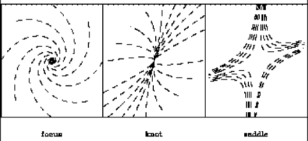
Figure 1: Classification of singular points. Field of polarization around singular points $p=0$. Dashed lines show the direction of the pseudo-vector $\overline{P}$ (but not its value). Left - focus, middle - knot, right - saddle.

This equation has two roots: $\lambda_{1}$ and $\lambda_{2}$, ordered by $Re(\lambda_{1})>Re(\lambda_{2})$, and the classification of the singular point $(x_{0},y_{0})$ depends on their values.
1. If $Im(\lambda_{1})=-Im(\lambda_{2})\neq 0$, then this is a focus and the vector field will spiral toward the point $(x_{0},y_{0})$ (Fig.1 left).
2. If $\lambda_{1}$ and $\lambda_{2}$ are real, then the matrix $M$ has two eigenvectors which correspond to different values $\lambda_{1}$ and $\lambda_{2}$, and we can consider two different cases:

a). $\lambda_{2}>0$ - both values are positive or $\lambda_{1}<0$ - both values are negative. This means, that the point $(x_{0},y_{0})$ is a knot and the lines of the vector field tend to be aligned to the direction of the eigenvector with maximal value of $|\lambda_{i}|$, $i=1,2$ (Fig.1 middle).

b). $\lambda_{1}>0$ and $\lambda_{2}<0$ - values with opposite signs. In this case the point $(x_{0},y_{0})$ is a saddle (Fig.1 right).

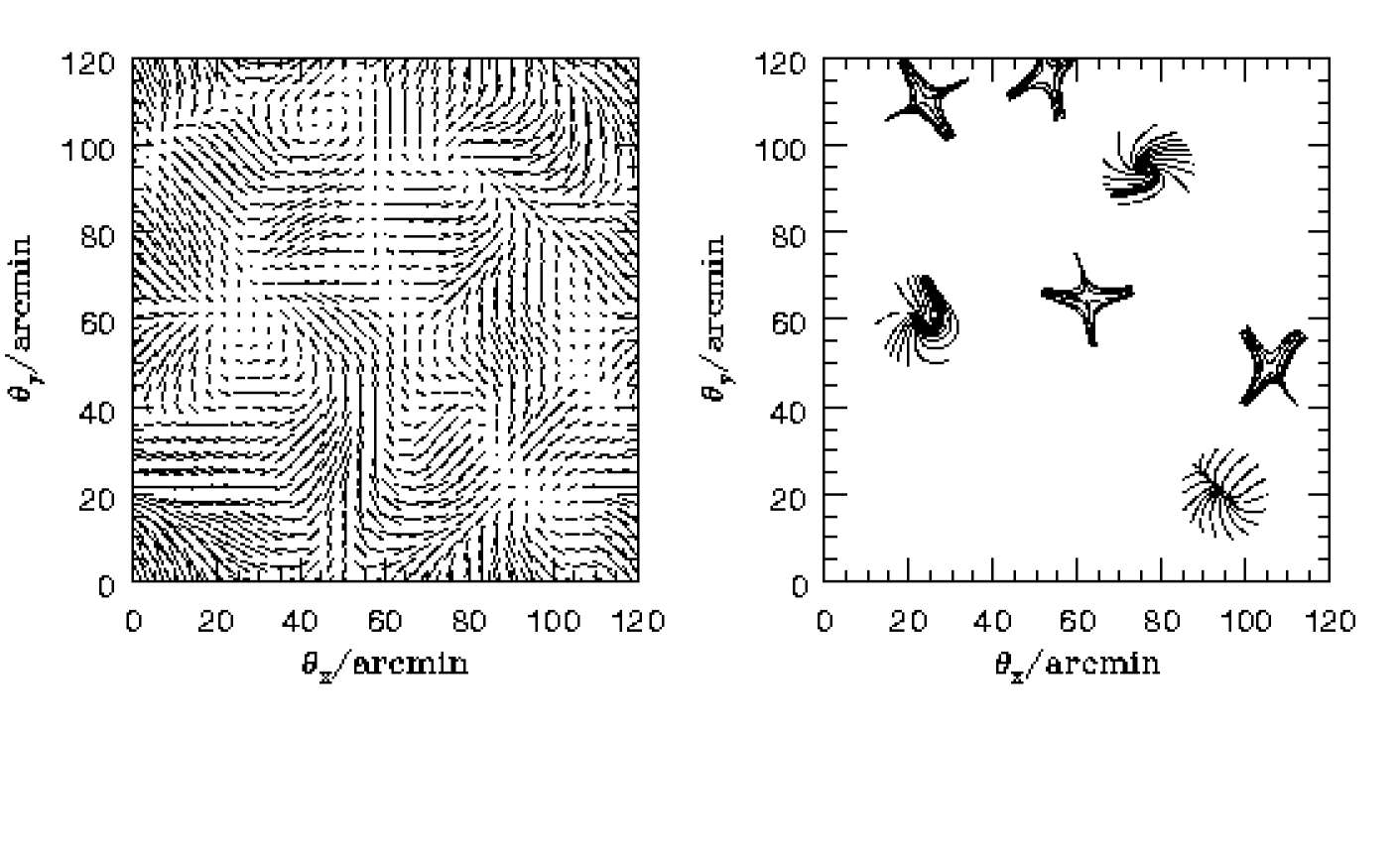
Figure 2: Simulated map $2^{0}\times 2^{0}$ of the CMB polarization field for the scale-invariant adiabatic CDM model with $\Omega=1$, $\Omega_{b}=0.03$, h=0.75 with smoothing angle 5 arcmin (FWHM). The simulation technique for small parts of the sky and spectrum for simulations are from Bond and Efstaphiou 1987.          Left - polarization field. The length of each vector is proportional to the degree of polarization and the orientation gives the plane of polarization. For visual clarity, we only use $50\times 50$ vectors.          Right - the same as left, but we plot only the orientation of polarization in the vicinity of non-polarized points (solid lines). This map containes 7 non-polarized points - 2 foci, 1 knot and 4 saddles.

Singular points of different types determine the behavior of the vector field in their vicinities. The distribution of the singular points on the map of cosmic microwave background polarization determines the topology of the relatively small polarized zones Fig.2.

b. Surface density of the singular points.

Detailed calculation of the surfase density of the singular points is in the Appendix A. The surface density of singular points of different kinds are:

$$\begin{array}[]{l}N_{f}=\frac{\sqrt{2}}{16\pi}\frac{1}{r_{c}^{2}},\\ N_{k}=\frac{\sqrt{2}}{16\pi}\left(\sqrt{2}-1\right)\frac{1}{r_{c}^{2}},\\ N_{s}=\frac{1}{8\pi r^{2}_{c}},\\ \end{array}$$ (12)

where $N_{f}$, $N_{k}$, $N_{s}$ are the number densities of focuses, knots and saddles respectively and $r_{c}=\frac{\sigma_{0}}{\sigma_{1}}$ is the correlation radius. The total number density of non-polarized points is:

$$N_{np}=N_{f}+N_{k}+N_{s}=\frac{1}{4\pi r_{c}^{2}}.$$ (13)

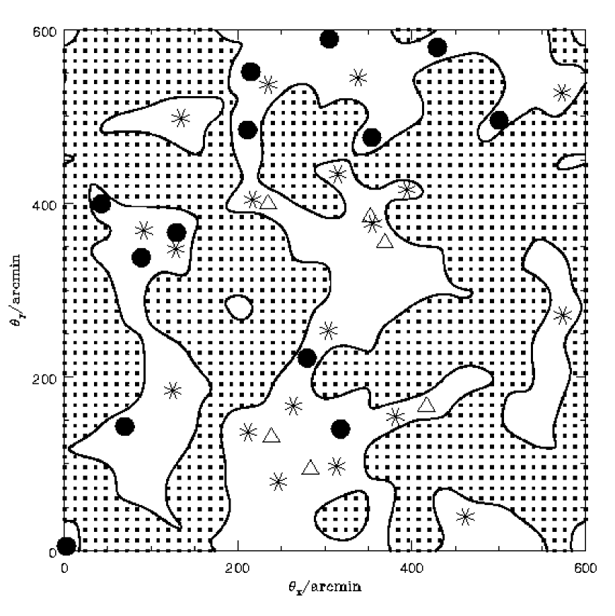
Figure 3: Simulated map $10^{0}\times 10^{0}$ of CMB polarization for the same model as in the fig. 2. Dashed area corresponds to the regions with polarization degree $p>p_{t}$. Solid lines are the boundary between regions with $p>p_{t}$ and $p<p_{t}$. Circles, threangles and stars are foci, knots and saddles correspondingly. This map containes 13 fosi, 6 knots and 19 saddles.

Density of the singular points depends essentially on correlation radius (Eq. 12, 13) and therefore on the spectral parameters $\sigma_{0}$, $\sigma_{1}$. These spectral parameters depend on the spectra of polarization and on the device resolution (Bond and Efstathiou, 1987) (see also Fig.3). The ratios

$$N_{f}/N_{k}=\sqrt{2}+1\hskip 28.45274ptand\hskip 28.45274ptN_{f}/N_{s}=\frac{\sqrt{2}}{2}$$ (14)

are the spectral independent constants determined only by the Gaussian nature of the primordial inhomogeneity in the Universe. These ratios are a characteristic feature of the CMB polarization vector field in the inflationary cosmology. Note, that for example in the two-dimensional potential vector field ($\overline{V}=\bigtriangledown\alpha$) the number density of foci is equal to zero since this field does not have a rotational component.

The joint probability for the distribution of the eigenvalues of $\lambda_{1}$ and $\lambda_{2}$ in the singular points which can be either knots or saddles (not foci) is:

$$F(\lambda_{1},\lambda_{2})d\lambda_{1}d\lambda_{2}=\frac{8}{4-\sqrt{2}}\frac{1}{\sqrt{\pi}}|\lambda_{1}\lambda_{2}|(\lambda_{1}-\lambda_{2})e^{-\frac{\lambda_{1}^{2}}{2}-\frac{\lambda_{2}^{2}}{2}}d\lambda_{1}d\lambda_{2}.$$ (15)

Note, that this distribution is universal for all kinds of spectra of polarization as well as ratios (15).

2.2 Percolation pattern for polarization

Here we present our results for the Genus statistics of the value $p=\frac{|\overline{P}|}{\sigma_{0}}$. We can divide the map of polarization of the CMB into two parts: regions with relatively strong polarization $p>p_{0}$ (“strongly polarized zones”) and regions with relatively weak polarization $p<p_{0}$ (“weakly polarized zones”). Below we find the value $p_{0}$ where percolation through the “strongly polarized zones” changes to percolation through the “weakly polarized zones” (Fig. 3,4). Let us suppose that we can measure only a signal with polarized intensity $p\geq p_{t}$, where $p_{t}$ is the threshold which determines by the sensitivity of the device. If we can measure only ”strongly polarized” signal - $p_{t}>p_{0}$, then we can see only the separated polarized spots which do not percolate. Therefore, the percolation trough polarized zones can be reached only by the device with the sensitivity $p_{t}\leq p_{0}$.

The value $p_{0}$ can be found analytically in the following way. We consider the value $|\overline{P}|$ as a two-dimensional random scalar field with a Rayleigh distribution (Coles and Barrow, 1987). This field can be imagined as a two-dimensional surface in a three-dimensional space. This surface has extreme points such as maxima, minima, saddle points and singular points. The last ones have been considered in the previous subsection. The densities of maxima, minima and saddle points have some distributions with $p$:

$$\begin{array}[]{l}N_{max}(p)=\int\limits_{p}^{\infty}n_{max}(p^{\prime})dp^{\prime},\\ N_{min}(p)=\int\limits_{p}^{\infty}n_{min}(p^{\prime})dp^{\prime},\\ N_{sad}(p)=\int\limits_{p}^{\infty}n_{sad}(p^{\prime})dp^{\prime},\end{array}$$ (16)

where $n_{max}(p)$, $n_{min}(p)$, $n_{sad}(p)$ - are the number densities of maxima, minima and saddle points respectively on some interval - (p,p+dp), and $N_{max}(p)$, $N_{min}(p)$, $N_{sad}(p)$ are the number densities of maxima, minima and saddle points respectively above some level $p$. (We note, that here saddle points are the saddle points of the two-dimensional surfase of p(x,y). These points are not the same as saddle (kind of singular points) in the previous section.)
The definition of the Genus is:

$$g(p)=n_{max}(p)+n_{min}(p)-n_{sad}(p).$$ (17)

The integrated Genus is then:

$$G(p)=N_{max}(p)+N_{min}(p)-N_{sad}(p)=\int\limits_{p}^{\infty}g(p^{\prime})dp^{\prime}.$$ (18)

The level of percolation $p_{0}$ has to be found from the condition $G(p_{0})=0$. We recognize that this condition does not automatically mean that $p_{0}$ is the level of percolation for an arbitrary scalar field. It is well-known that for the Gaussian random field the percolation level corresponds to the level where Genus curve intersects the zero. We have checked this condition for the Rayleigh distribution by simulating a large number of realizations for a two-dimensional field. In the case of Rayleigh distribution this condition also mean that level $p_{0}$ corresponds to the percolation contour.

The detailed calculation of the Genus can be found in Appendix B. Formally the steps of its calculation are as follows:
1. The value $p$ is a combination of the independent random values $q$ and $u$. The first and second derivatives of them are: $q_{i}$, $u_{i}$, $q_{ij}$, $u_{ij}$, ($q_{ij}=Q_{i,j}/\sigma_{2},u_{ij}=U_{ij}/\sigma_{2}$), $i=1,2$, where $\sigma_{2}$ is also the spectral parameter as it was defined by Bond and Efstaphiou 1987: $\sigma_{2}^{2}=\langle Q_{ii}^{2}\rangle=\langle U_{ii}^{2}\rangle$. These values obey the following conditions:

$$\begin{array}[]{l}p^{2}=q^{2}+u^{2}\\ p_{i}=qq_{i}+uu_{i},\\ \gamma p_{i}p_{j}+p_{ij}=\gamma(q_{i}q_{j}+u_{i}u_{j})+qq_{ij}+uu_{ij},\\ \langle qu\rangle=\langle q_{i}u_{j}\rangle=\langle q_{ij}u_{kl}\rangle=\langle qu_{i}\rangle=\langle q_{i}u\rangle=0,\\ \langle qq_{ij}\rangle=\langle uu_{ij}\rangle=-\frac{\gamma}{2}\delta_{ij},\\ \langle q_{i}q_{j}\rangle=\langle u_{i}u_{j}\rangle=\frac{1}{2}\delta_{ij},\\ \langle q_{ij}u_{kl}\rangle=\frac{1}{8}(\delta_{ik}\delta_{jl}+\delta_{il}\delta_{jk}+\delta_{ij}\delta_{kl}),\\ \gamma=\frac{\sigma_{1}^{2}}{\sigma_{0}\sigma_{2}}\end{array}$$ (19)

2. The joint probability F of the Gaussian distribution for the values $q$, $q_{i}$, $q_{ij}$, $u$, $u_{i}$, $u_{ij}$ is:

$$\begin{array}[]{l}Fdqdudq_{i}du_{i}dq_{ij}du_{ij}=\frac{1}{\sqrt{(2\pi)^{12}\det M}}e^{-\frac{A}{2}}dqdudq_{i}du_{i}dq_{ij}du_{ij},\\ A=v\times M^{-1}\times v^{T}\end{array}$$ (20)

where $M$ is the covariance matrix and A is the quadratic form of the 12-dimensional vector $v=(q,q_{i},q_{ij},u,u_{i},u_{ij})$.

3. The substitution of $p$, $p_{i}$, $p_{ij}$ in Eq.(20) from Eq.(19) and integration over 6 variables gives us the joint probability $fdpdp_{i}dp_{ij}$ for values $p$, $p_{i}$, $p_{ij}$ to be in the range from $p$, $p_{i}$, $p_{ij}$ to $p+dp$, $p_{i}+dp_{i}$, $p_{ij}+dp_{ij}$.

4. The differential density of the extreme points obeys the equation:

$$n_{ext}(p)=\frac{\sigma_{2}^{2}}{\sigma_{1}^{2}}\int|\det(p_{ij})|f\delta(p_{1})\delta(p_{2})dp_{ij},$$ (21)

where $n_{ext}(p)$ is the density of the extreme points. These extreme points can be maxima, minima or saddle points depending on the limits of the integration over $du_{ij}$. These limits determine by the values of $tr(p_{ij})$ and $det(p_{ij})$ of the second derivatives matrix $(p_{ij})$ (see Appendix B).

5. The Genus curve obeys the equation:

$$g(p)=n_{max}(p)+n_{min}(p)-n_{sad}(p)=\frac{\sigma_{2}^{2}}{\sigma_{1}^{2}}\int\det(p_{ij})f(p,p_{i}=0,p_{ij})dp_{ij}.$$ (22)

After integrating this, we have

$$g(p)=\frac{1}{4\pi}\left(\frac{\sigma_{1}}{\sigma_{0}}\right)^{2}p(p^{2}-3)e^{-\frac{p^{2}}{2}}.$$ (23)

The integrated Genus curve is

$$G(p)=\frac{1}{4\pi r_{c}^{2}}(p^{2}-1)e^{-\frac{p^{2}}{2}},$$ (24)

Condition $G(p)=0$ gives us the value of $p_{0}$:

$$p_{0}=1.$$ (25)

Taking into account that random value $p$ has distribution $pe^{-\frac{p^{2}}{2}}dp$ we can obtain that percolation through the “strongly polarized” zone when a part $e^{-\frac{p^{2}_{0}}{2}}$ of the map is detected as a “strongly polarized”. This corresponds to $\approx 61\%$ of the map’s area.

When $p_{0}=0$ in Eq.(25) we have

$$g(0)=-\frac{1}{4\pi r_{c}^{2}}.$$ (26)

This value exactly coincides with $N_{np}$ in Eq. (13) with the opposite sign. These null-points are the non-smooth minima of the surface $p$. The non-smooth minima have not been taken into account in Eqs.(16)-(25). Therefore, the total number of minima per unit area is $N_{mintotal}=N_{np}+N{min}(0)$, where $N_{np}$ are minima, if p=0 and $N_{min}(0)$ are minima, if p¿0. Therefore the total number of extreme points per unit area are:

$$\begin{array}[]{l}N_{maxtotal}=N_{max}(0),\\ N_{sadtotal}=N_{sad}(0),\\ N_{mintotal}=N_{np}+N{min}(0).\end{array}$$ (27)

Taking into account equations (13,18,25,27) we obtain:

$$N_{maxtotal}+N_{mintotal}-N_{sadtotal}=0,$$ (28)

as it should be.

3 Minkowski functionals for CMB polarization field

As it was mentioned above, the CMB polarization at any point of the map can be characterized by the orientation angle and polarized intensity - p. This intensity has the random Rayleigh distribution on the sky - $p=\sqrt{q^{2}+u^{2}}$. Therefore, the value of $p$ can be considered as a two-dimensional random Raleigh field. It is well-known, that two-dimensional field has only three Minkowski functionals which satisfy additivity and translational invariance (Minkowski 1903, Hadwiger 1959).

Geometrical interpretation of the Minkowsky functionals on the two-dimensional map is essentially easy. Analogously to the previous section, we consider polarized intensity as a two-dimensional surface in a three-dimensional space. If we cut this surface at the different levels $p_{t}$, then the area of the map will be divided into two parts: the area, where polarization is above the threshold $p_{t}$ and the area, where $p<p_{t}$. For a two-dimensional distribution, Minkowski functionals correspond to the following values:
1. A - fraction of the area of the map, where $p>p_{t}$;
2. L - length of the boundary between fractions, where $p>p_{t}$ and $p<p_{t}$ per unit area;
3. $G=N_{max}+N_{min}-N_{sad}$ - Euler characteristic (equivalent to the genus) per unit area.

Therefore, threshold is the independent variable on which these functionals depend. The third functional has already been considered in the previous section. The obvious first one is $e^{-\frac{p_{t}^{2}}{2}}$. The second one can be obtained in the same way as it was done for the the Gaussian field (Adler 1981). Here we present the result without derivation:

$$L=\frac{1}{r_{c}}p_{t}e^{-\frac{p_{t}^{2}}{2}}$$ (29)

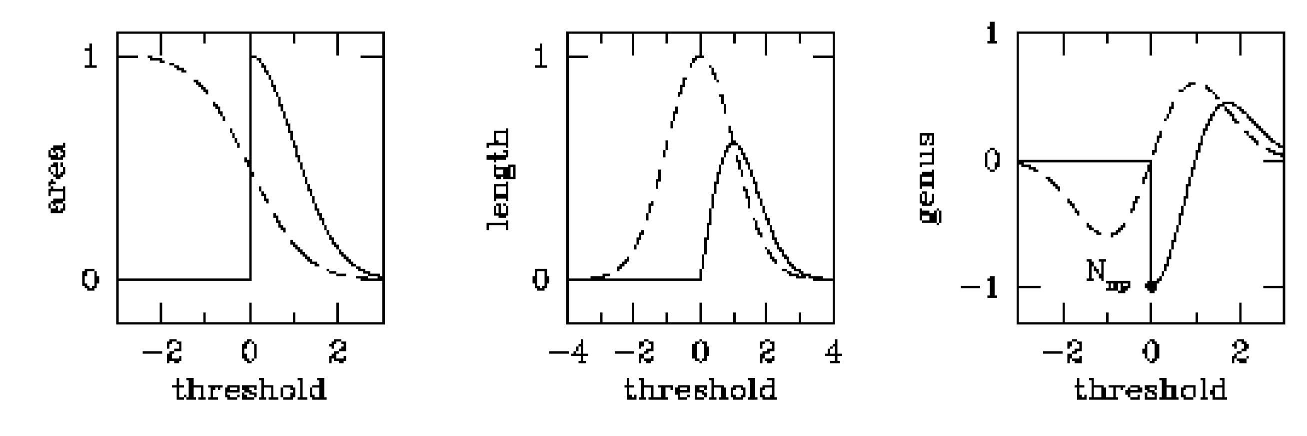
Figure 5: Minkowski functionals for CMB polarization (solid lines) and anisotropy (dashed lines). Threeshold is given in the units of $\sigma_{0}$ for polarization and in the units of $\sqrt{\langle(\Delta T)^{2}\rangle}$ for anisotropy.

The comparison of the Minkowski functionals for the CMB polarization field with these functionals for CMB anisotropy is in the Fig. 5. Functionals for Rayleigh distribution are equal to zero for $p_{t}<0$. The third functional should be described together with the number of non-polarized points (see previous section). These functionals can be used as a morphological descriptor of the CMB polarization field in a similar manner as for the CMB anizotropy (Winitski and Kosowski 1997).

4 Discussions

In this paper we have presented calculations of the statistical properties CMB polarization maps.

We believe that these statistical properties can be useful for checking the polarization patterns for presence of the non-Gaussian noise (for example, confusion signal from sources which can have the same spectral parameters as the polarization of the CMB). If an observational signal is free from non-Gaussian noise and is Gaussian itself (due to inflation) then the topological approach is not necessary, because the correlation function or equivalent its power spectrum contains all information about the polarization signal. On the other hand, if the signal is a sum of polarization of the CMB (which is Gaussian) and unresolved foreground sources (which are non-Gaussian), then a detailed topological picture of the polarization field around the non-polarization points will be distorted comparative the predictions of the theory for the Gaussian distributions.

On the other hand, the investigation of the nature of the primordial polarized signal is a test of the inflationary model of the evolution of the Universe. Therefore, the investigation of the Minkowski functionals together with the non-polarized points on the observational data and comparison with the theoretical predictions can be used as the test on Gaussianity of the primordial inhomogeneity.

We would like to emphasize that the regions with strong polarization will be detected easier than the regions with weak polarization. As we demonstrated in the paper (see section 2.2) these region occupy an essential part of a whole map. From this point of view it is interesting to study the statistical properties of these regions. It is worth also mentioning that it is interesting to investigate the dependence of the spectral parameters of polarization in various cosmological models on the resolution of the detector and related statistical properties of the maps of polarization of the CMB. It is also very interesting to stady the cross-correlations between anisotropy and polarization on the sky map and make some theoretical predictions from the geometrical point of view. These quations will be considered in a separate paper.

We would like to thank A. Melott, I. Novikov and S.Shandarin for stimulating discussion. At the University of Kansas the research was supported by NSF-NATO fellowship (DGE-9710914) and by the NSF EPSCOR program. We are grateful to the staff of TAC, and the Copenhagen University Observatory for providing excellent working conditions. This investigation was supported in part by the Russian Foundation for Fundamental Research (Code 96-02-17150) and by a grant ISF MEZ 300 as well as by the Danish Natural Science Research Council through grant No. 9401635 and also in part by Danmarks Grundforskningsfond through its support for the establishment of the Theoretical Astrophysics Center.

Appendix A

Surface density of the singular points

Below we describe the density of foci, knots and saddles. The total density of singular (non-polarized) points is:

$$N_{np}=\frac{4}{(2\pi)^{3}}\left(\frac{\sigma_{1}}{\sigma_{0}}\right)^{2}\int|q_{1}u_{2}-u_{1}q_{2}|e^{-\frac{A}{2}}dq_{i}du_{i},\hskip 122.34692pt(A1)$$

where

$$A=\sum\limits_{i=1,2}2q_{i}^{2}+2u_{i}^{2},\hskip 14.22636pti=1,2.$$

The substitution

$$\begin{array}[]{ll}q_{1}=\frac{1}{2}(x+R\cos\varphi),&u_{1}=\frac{1}{2}(w+R\sin\varphi),\\ q_{2}=\frac{1}{2}(R\sin\varphi-w),&u_{2}=\frac{1}{2}(x-R\cos\varphi),\\ \end{array}\hskip 136.5733pt(A2)$$

and integration over $d\varphi$ gives us:

$$N_{np}=\frac{1}{4}\frac{1}{(2\pi)^{2}}\left(\frac{\sigma_{1}}{\sigma_{0}}\right)^{2}\int e^{-\frac{1}{2}(x^{2}+R^{2}+w^{2})}|x^{2}+w^{2}-R^{2}|R\ dRdxdw.\hskip 28.45274pt(A3)$$

The next substitution $b=R^{2}-w^{2}$ allows us to rewrite (A3) in the following form:

$$N_{np}=\frac{1}{8}\frac{1}{(2\pi)^{2}}\left(\frac{\sigma_{1}}{\sigma_{0}}\right)^{2}\int e^{-\frac{1}{2}x^{2}}dx\int e^{-w^{2}}dw\int|x^{2}-b|e^{-\frac{b}{2}}db\hskip 56.9055pt(A4)$$

where $-w^{2}<b<\infty$, $-\infty<x<+\infty$, $-\infty<w<+\infty$. In terms of $x$ and $b$ the eigenvalues of the matrix

$$M=\left(\begin{array}[]{ll}q_{1}&q_{2}\\ u_{1}&u_{2}\end{array}\right)\hskip 270.30118pt(A5)$$

are

$$\lambda_{1,2}=\frac{1}{2}(x\pm\sqrt{b}).\hskip 275.99164pt(A6)$$

From (A4, A6) we can obtain the density of focuses, saddles and knots:

$$\begin{array}[]{lll}-w^{2}<b<0&-&foci\\ 0<b<x^{2}&-&knots\\ x^{2}<b<\infty&-&saddles\end{array}\hskip 221.93158pt(A7)$$

Using (A4), (A7) we obtain

$$\begin{array}[]{l}N_{f}=\frac{\sqrt{2}}{16\pi}\left(\frac{\sigma_{1}}{\sigma_{0}}\right)^{2}\\ N_{k}=\frac{1}{16\pi}(2-\sqrt{2})\left(\frac{\sigma_{1}}{\sigma_{0}}\right)^{2}\\ N_{s}=\frac{1}{8\pi}\left(\frac{\sigma_{1}}{\sigma_{0}}\right)^{2}\\ \end{array}\hskip 233.3125pt(A8)$$

Using (A4, A6-A8) the joint probability for values $\lambda_{1}$, $\lambda_{2}$ in the peculiar points which can be knots or saddles (not focuses) is

$$P(\lambda_{1},\lambda_{2})d\lambda_{1}d\lambda_{2}=\frac{8}{(4-\sqrt{2})\sqrt{\pi}}|\lambda_{1}\lambda_{2}|(\lambda_{1}-\lambda_{2})e^{-\lambda_{1}^{2}-\lambda_{2}^{2}}d\lambda_{1}d\lambda_{2},\hskip 5.69046pt\lambda_{1}>\lambda_{2}.\hskip 14.22636pt(A9)$$

Appendix B

Genus curve

In this appendix we obtain the differential and integrated Genus curve for the two-dimensional random Rayleigh field.

According to section 2.2 the value $P=\sqrt{q^{2}+u^{2}}$ is the non-linear combination of two different independent random Gaussian fields $q$ and $u$. Equation (17) for the joint probability distribution of the values $q$, $u$, $q_{i}$, $u_{i}$ $q_{ij}$, $u_{ij}$, $i,j=1,2$ contains the quadratic form $A$ and $\det M$, where $M$ is a covariance matrix:

$$\begin{array}[]{l}A=q^{2}+u^{2}+2(q_{1}^{2}+q_{2}^{2}+u_{1}^{2}+u_{2}^{2})+\frac{(q_{11}+q_{22}+\gamma q)^{2}+(u_{11}+u_{22}+\gamma u)^{2}}{1-\gamma^{2}}+\\ +2(q_{11}-q_{22})^{2}+2(u_{11}-u_{22})^{2}+8q^{2}_{12}+8u^{2}_{12},\\ \det M=2^{-12}(1-\gamma^{2})^{2}.\\ \end{array}\hskip 34.14322pt(B1)$$

The substitutions in Eq.(17)

$$\begin{array}[]{ll}q=p\cos\varphi,&u=p\sin\varphi,\\ p_{i}=q_{i}\cos\varphi+u_{i}\sin\varphi,&l_{i}=q_{i}\sin\varphi-u_{i}\cos\varphi,\\ l_{ij}=q_{ij}\cos\varphi+u_{ij}\sin\varphi,&\tilde{l}_{ij}=q_{ij}\sin\varphi-u_{ij}\cos\varphi,\\ i,j=1,2,&\\ \end{array}\hskip 108.12054pt(B2)$$

and integration over $dl_{i}d\tilde{l}_{ij}$ gives us the joint probability for the distribution of the values $p$, $p_{i}$, $l_{i}$, $l_{ij}$:

$$X(p,p_{i},l_{i},l_{ij})dpdp_{i}dl_{i}dl_{ij}=\frac{32}{(2\pi)^{7/2}(1-\gamma^{2})^{1/2}}pe^{-\frac{\tilde{A}}{2}}dpdp_{i}dl_{i}dl_{ij}\hskip 2.84544pti,j=1,2\hskip 8.5359pt(B3)$$

Following Eqs.(16) and (B2) we can get the expression:

$$pp_{ij}=pl_{ij}+\gamma l_{i}l_{j};\hskip 284.52756pt(B4)$$

using Eqs.(20), (B3) and (B4) we obtain

$$g(p)=\frac{32}{(2\pi)^{7/2}(1-\gamma^{2})^{1/2}}\int(p_{11}p_{22}-p_{12}^{2})pe^{-\frac{\tilde{\tilde{A}}}{2}}dl_{i}dp_{ij}\hskip 14.22636pti,j=1,2$$

$$\tilde{\tilde{A}}=p^{2}+2(l_{1}^{2}+l_{2}^{2})+\frac{(p_{11}+p_{22}-\gamma a)^{2}}{1-\gamma^{2}}+2(p_{11}-p_{22}-\gamma b)^{2}+8(p_{12}-\gamma c)^{2}\hskip 28.45274pt(B5)$$

$$a=\frac{l_{1}^{2}+l_{2}^{2}}{p}-p,\hskip 14.22636ptb=\frac{l_{1}^{2}-l_{2}^{2}}{p}\hskip 14.22636ptc=\frac{l_{1}^{2}l_{2}^{2}}{p}$$

the integration over $dp_{ij}$, $dl_{i}$ gives us differential Genus curve

$$g(p)=\frac{1}{4\pi}\left(\frac{\sigma_{1}}{\sigma_{0}}\right)^{2}p(p^{2}-3)e^{-\frac{p^{2}}{2}}\hskip 227.62204pt(B6)$$

The integrated curve is

$$G(p)=\int\limits^{\infty}_{p}g(p^{\prime})dp^{\prime}=\frac{1}{4\pi}\left(\frac{\sigma_{1}}{\sigma_{0}}\right)^{2}(p^{2}-1)e^{-\frac{p^{2}}{2}}.\hskip 150.79968pt(B7)$$

REFERENCES

Adler, R.J., The geometry of random fields, John Wiley & Sons, Chichester, 1981.
Arbuzov P., Kotok E., Naselsky P. and Novikov I., 1997a, Preprint TAC, 1997-017, Intern. J.of Mod.Physics (submitted)
Arbuzov P., Kotok E., Naselsky P. and Novikov I., 1997b, Preprint TAC, 1997-021, Intern. J.of Mod.Physics (submitted).
Bardeen,J.M.,Bond,J.R.,Kaiser,N.,& Szalay, A.S., Ap.J. 304,(1986) 15-61.
Basco M.A., Polnarev A.G., Sov. Astron., 1979, 24, 3
Bennett C.L., et al, 1996, ApJ. 464, L1.
Bond J.R., G. Efstathiou., 1987, M.N.R.A.S. 336, 655
Cheng E.S., et al, 1994, ApJ. 422, L37
Coles,P.& Barrow,J.D., 1987, M.N.R.A.S 228, 407-426
Coles,P. M.N.R.A.S, 1988, 231, 125-130
Coulson P., Grittenden. R., Turok N., 1994, Phys. Rev. Lett., 73, 2390
Dominik, K., & Shandarin, S. 1992, ApJ, 393, 450
Doroshkevich,A.G.,Astrophysics 6 (1970), 320-330
De Bernardis. P., et al, 1994, ApJ. 422, L33
Grittenden R. Coulson P., Turok N., 1995, Phys. Rev. D, 52, 5402
Hadwiger,H., Vorlesungen uber Inhalt, Oberflache und Isoperimetrie, Springer Verlag, Berlin, 1957
Harari,D.D., & Zaldarriaga, M. 1993, Phys. Letters B, 319, 96
Harari,D.D., Hayward,J.D., & Zaldarriaga, M. 1996, Phys. Rev. D, 55, 1841
Hancock S., et al, 1994, Nature 367, 333.
Hu. W and M.White, 1997, astro-ph 970647
Jungman G., Kamionkowski M.A. Kosowsky A., D. Spergel, 1996, Phys. Rev. D, 54, 1332
Kamionkowski M.A. Kosowsky A. and Stebbins A., 1997, Phys. Rev. D 55, 7368
Keating, B., Polnarev, A., Steinberger, J., Timbie, P., (1987) astro-ph
Kogut,A. et al. 1994, ApJ, 433, 435
Kosowsky A., 1996, Annals Phys. 246, 49
Luo, X. & Schramm, D.N. 1994, Phys. Rev. Lett., 71, 1124
Masi S. et al, 1996, ApJ. 463, L47
Melott, A.L. 1990, Phys. Reports, 193, 1
Minkowski,H., Mathematische Annalen 57 (1903), 447-495
Naselsky P. and Novikov D., 1995, ApJ. 444, L1
Naselsky P.D. and Polnarev A.G., 1987, Astrophysica 26, 543
Netterfield et al., 1996, astro-ph 9601197
Novikov D. and H. Jørgensen, 1996a, ApJ. 471, 521
Novikov D. and H. Jørgensen, 1996b, Intern. J.of Mod.Physics 5, 319
Ng K.L. and Ng K.W., 1995, Phys. Rev. D, 51, 364
Ng K.L. and Ng K.W., 1996, ApJ. 456, L1
Polnarev A.G., 1985, Sov. Astron., 1979, 62, 1041
Rees M., 1968, ApJ. 153, L1
Scott,D., Silk,J., & White,W. 1995, Science, 268, 829
Scott P.F., et al, 1996, ApJ. 461, L1
Schmalzing J., Gorski K.M., astro-ph/9710185
Seljak, U., & Zaldarriaga, M. Ap.J., (1996), 469, 437
Seljak, U., & Zaldarriaga, M. Ap.J., (1996), astro-ph 9609169
Shandarin, S.F. 1983, Soviet Astron. Lett., 9, 104
Smoot G., et al., 1992, ApJ. Lett. 396, L1
Smoot G., et al., 1994, ApJ. 437, 1
Tanaka et al. 1995, astro-ph 9512067
Torres, S., et al., 1995, MNRAS, 274, 853-857
Winitzki, S., & Kosowsky, A. (1997) astro-ph/9710164
Zaldarriaga, M., Harari, D., 1995, Phys. Rev. D, 52, 3276
Zaldarriaga, M., & Seljak, U., 1997, Phys. Rev. D, 55, 1830
Zaldarriaga, M. 1997, Phys. Rev. D, 55, 1822
Zeldovich, Ya.B. 1982, Soviet Astron. Lett., 8,102.

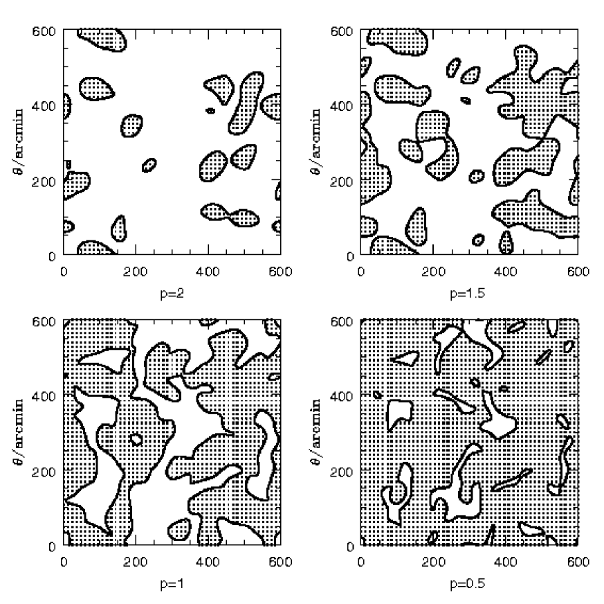
Figure 4: The same as in fig. 3, but without non-polarized points. We plot area, where $p>p_{t}$ for different values of $p_{t}$: $p_{t}=2,1.5,1,0.5$. Spots with $p>p_{t}$ percolate then $p_{t}=1$, which corresponds to the $e^{-1/2}\sim 61\%$ of the maps area.