Mock 2dF and SDSS galaxy redshift surveys

Abstract

We present a comprehensive set of mock 2dF and SDSS galaxy redshift surveys constructed from a set of large, high-resolution cosmological $N$-body simulations. The radial selection functions and geometrical limits of the catalogues mimic those of the genuine surveys. The catalogues span a wide range of cosmologies, including both open and flat universes. In all the models the galaxy distributions are biased so as to approximately reproduce the observed galaxy correlation function on scales of $1$–$10h^{-1}\,{\rm Mpc}$. In some cases models with a variety of different biasing prescriptions are included. All the mock catalogues are publically available at http://star-www.dur.ac.uk/$\tilde{\hphantom{g}}$cole/mocks/main.html . We expect these catalogues to be a valuable aid in the development of the new algorithms and statistics that will be used to analyse the 2dF and SDSS surveys when they are completed in the next few years. Mock catalogues of the PSCZ survey of IRAS galaxies are also available at the same WWW location.

1 Introduction

Our knowledge of large scale stucture in the Universe is going to change dramatically as a result of the new generation of galaxy redshift surveys now underway. The Anglo-Australian 2-degree Field (2dF) galaxy redshift survey will measure redshifts for 250,000 galaxies selected from the APM galaxy survey (Maddox et al. 1990), and the Sloan Digital Sky Survey (SDSS) will obtain a redshift sample of one million galaxies. These surveys will be more than one order of magnitude larger than any existing survey and will allow measurements of large-scale structure of unprecedented accuracy and detail. Precise estimates of the standard statistics that are used to quantify large-scale structure (e.g., the galaxy correlation function $\xi(r)$ and power spectrum $P(k)$) will be possible, and the surveys will provide the first opportunity to examine more subtle properties of the galaxy distribution. Achieving these goals will require the development of faster algorithms capable of dealing with the very large numbers of galaxies involved, and the development of new statistical measures. To facilitate both of these tasks before the surveys are complete will require synthetic data sets on which the techniques can be developed and tested.

This paper presents an extensive set of mock 2dF and SDSS galaxy catalogues. These artificial galaxy redshift catalogues have been constructed from a series of large, high-resolution cosmological $N$-body simulations. The $N$-body simulations span a wide range of cosmological models, with varying values of the density parameter, $\Omega_{0}$, and the cosmological constant, $\Lambda_{0}$, and with varying choices of the shape and amplitude of the mass fluctuation power spectrum, $P(k)$. For some models several different catalogues have been produced, each employing a different biasing algorithm to relate the galaxy distribution to the underlying mass distribution. All the mock galaxy catalogues have selection functions that mimic those expected for the real surveys. The details of the construction of catalogues and their basic properties are described here. The catalogues themselves can be obtained from http://star-www.dur.ac.uk/$\tilde{\hphantom{g}}$cole/mocks/main.html .

The mock redshift catalogues are the principal scientific product of this paper. We expect to use them ourselves as we prepare for the analysis of large-scale structure in the 2dF and SDSS redshift surveys. We are making them publically available in the hope that they will be useful to other researchers, both inside and outside the two collaborations. Our illustrative plots also provide a qualitative prediction of the structure expected in these redshift surveys if the leading scenario for structure formation, based on Gaussian primordial fluctuations and a universe dominated by cold dark matter, is basically correct. The mock catalogues have a number of limitations (discussed in §6 below) — for example, the $345.6h^{-1}\,{\rm Mpc}$ simulation cubes are not as large as one might like, and we do not model some of the detailed selection biases that will affect the real surveys, such as loss of members of close galaxy pairs because of a minimum fibre separation. The strength of this collection of catalogues is that it covers a wide range of theoretically interesting cosmological models in a systematic, homogeneous, and documented fashion. We anticipate that these catalogues will be especially helpful to researchers who want to test the discriminatory power of statistical techniques that probe intermediate scale clustering ($\sim 1-100h^{-1}\,{\rm Mpc}$) and/or to develop practical implementations of these techniques for large data sets. Eventually, mock catalogues like these, or improved versions of them, will be a valuable tool for comparing the survey data against the predictions of cosmological theories.

The cosmological models we have selected fall into two sets, which we refer to as “COBE normalized” and “structure normalized” (or “cluster normalized”). In the COBE normalized models, the amplitude of the density fluctuations is set by the amplitude of the cosmic microwave background temperature fluctuations measured by the COBE satellite and extrapolated to smaller scales using standard assumptions. The shape of the spectrum of density fluctuations is fixed by applying additional constraints on the age of the universe and the baryon fraction. The structure normalized models are, on the other hand, intended to produce approximately the observed abundance of rich galaxy clusters, and all of them have the same shape for the density fluctuation spectrum, chosen to be consistent with existing observations of large-scale structure. Each set contains both open ($\Lambda_{0}=0$) and flat ($\Omega_{0}+\Lambda_{0}=1$) models with a range of values of $\Omega_{0}$. Some of the models we consider come close to satisfying simultaneously the COBE and cluster abundance constraints. For each simulation we apply a “biasing” algorithm to select galaxies from the $N$-body particle distribution, choosing its parameters so that the simulated galaxy population approximately reproduces the amplitude and slope of the observed galaxy correlation function on scales $\sim 1-10h^{-1}\,{\rm Mpc}$. For a few of the models we create multiple catalogues using several different biasing schemes, so that the sensitivity of methods to the detailed properties of biased galaxy formation can be investigated. The COBE normalized models arguably have a stronger theoretical motivation, since they represent the predictions of models that assume inflationary primordial fluctuations and cold dark matter with the specified values of $\Omega_{0}$, $\Lambda_{0}$, $\Omega_{\rm b}$, and the Hubble constant. Since the structure normalized CDM models all have the same spectral shape they are particularly useful for testing techniques designed to measure $\Omega_{0}$ or $\Lambda_{0}$ independently of an assumed shape of the primordial mass power spectrum. We have presented analyses of aspects of these simulations elsewhere ([1996]; Cole et al. 1997, hereafter []; [1998]).

The paper is structured in the following way. The choice and parameterization of the cosmological models is discussed in Section 2. Section 3 is a full description of all the details of our $N$-body simulations. The construction of the initial conditions and their evolution are described in Sections 3.1 and 3.2. The biasing prescriptions are explained in Section 3.3. The method by which the biased distributions are converted into mock galaxy catalogues is presented in Section 4. Our modelling of the survey geometries and selection functions is detailed in Section 4.2. Section 5 presents plots showing slices of the galaxy distributions in a selection of the mock galaxy catalogues. The qualitative differences that are discernible in these distributions and the processes that give rise to them are discussed. In Section 6 we discuss the limitations of our approach. Section 7 gives instructions on how to obtain and manipulate the mock galaxy catalogues. We conclude in Section 8 .

2 Cosmological Models

All our cosmological models are variants of the cold dark matter (CDM) scenario. The functional form we adopt for the matter power spectrum is that given by Bardeen et al. ([1986]),

$$P(k) \propto \frac{k^{n}}{\left[1+3.89q+(16.1q)^{2}+(5.46q)^{3}+(6.71q)^{4}\right]^{1/2}}$$ (2.1)

$$\times\frac{\left[\ln(1+2.34q)\right]^{2}}{(2.34q)^{2}},$$

where $q=k/\Gamma$ and $k=2\pi/\lambda$ is the wavenumber in units of $h{\rm Mpc}^{-1}$. The index $n$ is the slope of the primordial power spectrum, and in all but one case we adopt $n=1$, as predicted by the simplest models of inflation. Two further parameters complete the description of the matter power spectrum. These are the shape parameter $\Gamma$ and the amplitude of the power spectrum, which we specify through the value of $\sigma_{8}$, the linear theory rms fluctuation of the mass contained in spheres of radius $8h^{-1}\,{\rm Mpc}$. The background cosmological model in which these fluctuations evolve is specified by the density parameter $\Omega_{0}$ and the cosmological constant $\Lambda_{0}$, which we express in units of $3H_{0}^{2}/c^{2}$, where $H_{0}$ is the present value of the Hubble parameter. Thus, with the exception of the one tilted model with $n\neq 1$, our models are fully specified by the values of four parameters, $\Omega_{0}$, $\Lambda_{0}$, $\sigma_{8}$ and $\Gamma$. For each of our twenty models, Table 1 lists the values of these parameters along with other parameters that are described below. The names we have listed for the cosmological models are consistent with the convention used in [], but in addition we have included (in parentheses) some more descriptive names for the various $\Omega_{0}=1$ models.

Table 1: Simulation Parameters: the first column gives the label of each of the cosmological models; alternative, more descriptive names for the $\Omega_{0}=1$ models are given in parentheses. The following eight columns give the corresponding values of the density parameter $\Omega_{0}$, cosmological constant $\Lambda_{0}$, Hubble parameter $h$, age of the universe $t$, baryon content $\Omega_{\rm b}$, power spectrum shape parameter $\Gamma$, and normalization $\sigma_{8}$ respectively. The final two columns give the initial expansion factors, $a_{\rm i}$, and number of timesteps, $N_{\rm steps}$, used in the $N$-body simulation.

Model	$\Omega_{0}$	$\Lambda_{0}$	h	$t/{\rm Gyr}$	$\Omega_{\rm b}$	$\Gamma$	$\sigma_{8}$	$a_{\rm i}$	$N_{\rm steps}$
O3	0.3	0.0	0.65	12.2	0.030	0.172	0.5	0.15	93
O4	0.4	0.0	0.65	11.7	0.030	0.234	0.75	0.1	168
O5	0.5	0.0	0.6	12.3	0.035	0.27	0.9	0.08	254
L1	0.1	0.9	0.9	13.9	0.015	0.076	0.7	0.15	150
L2	0.2	0.8	0.75	14.0	0.022	0.131	0.9	0.12	220
L3	0.3	0.7	0.65	14.5	0.030	0.172	1.05	0.101	266
L4	0.4	0.6	0.6	14.5	0.035	0.213	1.1	0.09	275
L5	0.5	0.5	0.6	13.5	0.035	0.27	1.3	0.07	331
O2S	0.2	0.0	–	–	–	0.25	1.44	0.028	447
O3S	0.3	0.0	–	–	–	0.25	1.13	0.050	313
O4S	0.4	0.0	–	–	–	0.25	0.95	0.073	258
O5S	0.5	0.0	–	–	–	0.25	0.83	0.096	212
L2S	0.2	0.8	–	–	–	0.25	1.44	0.057	405
L3S	0.3	0.7	–	–	–	0.25	1.13	0.080	287
L4S	0.4	0.6	–	–	–	0.25	0.95	0.102	224
L5S	0.5	0.5	–	–	–	0.25	0.83	0.122	184
E1S (CCDM)	1.0	0.0	0.5	13.1	–	0.5	1.35	0.061	327
E2S (tilted)	1.0	0.0	0.5	13.1	0.05	–	0.55	0.20	200
E3S ($\tau$CDM)	1.0	0.0	–	–	–	0.25	0.55	0.21	103
E4S (SCDM)	1.0	0.0	0.5	13.1	–	0.5	0.55	0.15	170

The COBE -normalized set of models consists of an Einstein-de Sitter, $\Omega=1$, model (labelled E1 or CCDM for COBE normalized CDM), three open models with $\Omega_{0}=0.3$, $0.4$ and $0.5$ (labelled O3-O5) and five flat models with $\Omega_{0}=0.1$-$0.5$ and $\Omega_{0}+\Lambda_{0}=1$ (labelled L1-L5). We do not include COBE normalized open models with $\Omega_{0}=0.1$ or 0.2 because they are hopelessly inconsistent with the observed abundance of rich galaxy clusters ([]). For each of the open models we choose the value of the Hubble parameter $h$ that gives a universe of age $t\approx 12$Gyr, i.e. the largest value of $h$ that is consistent with standard globular cluster age estimates ([1996, 1996]; Salaris, Degl’Innocenti & Weiss [1997]). For each of the low-$\Omega_{0}$ flat models we choose the value of $h$ that gives $t\approx 14$Gyr. For $\Omega_{0}=1$ we take $h=0.5$. Having chosen these values of $h$, we fix the baryon fraction in these models using the constraint from primordial nucleosynthesis of $\Omega_{\rm b}=0.0125h^{-2}$ ([1991]). We then use the following expression for the shape parameter $\Gamma$,

$$\Gamma=\Omega_{0}h\,\exp(-\Omega_{\rm b}-\Omega_{\rm b}/\Omega_{0}),$$ (2.2)

which approximately accounts for the effect of baryons on the transfer function ([1995]). Finally, in each of these models the amplitude of the density perturbations is set so as to be consistent with the COBE measurements of fluctuations in the cosmic microwave background ([1992]). Further details of these models can be found in [], which examines the abundance of galaxy clusters in COBE normalized CDM and presents some analysis of clustering of the mass distributions.

For the set of structure normalized models, we adopt a fixed value of $\Gamma=0.25$, as suggested by observations of the large-scale structure traced by galaxies (e.g. [1990a]). The amplitude of the power spectrum we set according to the formula, $\sigma_{8}=0.55\Omega_{0}^{-0.6}$, which results in an abundance of rich galaxy clusters in good agreement with observations ([1993a]). These models include the Einstein-de Sitter model E3S (of which we have two realizations labelled E3S A and E3S B), a series of open models with $\Omega_{0}=0.2$-$0.5$ (labelled O2S-O5S), and a series of flat models with $\Omega_{0}=0.2$-$0.5$ and $\Omega_{0}+\Lambda_{0}=1$ (labelled L2S-L5S). Physically, these models could be produced either by having $h=\Gamma/\Omega_{0}$ or by a change from the standard model of the present energy density in relativistic particles. For example the E3S model is very similar to the $\tau$CDM model of Jenkins et al. ([1997]), which is motivated by the decaying particle model proposed by Bond & Efstathiou ([1991]). The final model listed in Table 1, E4 (SCDM), is the “standard” CDM model ($\Gamma=h=0.5$), normalized by the abundance of galaxy clusters.

We consider one further model that falls into both the COBE and structure normalized categories. This is the tilted Einstein-de Sitter model, E2 (tilted). For this model, the above constraints have been applied in relating the baryon fraction $\Omega_{\rm b}$, the Hubble parameter $h$, and the shape parameter $\Gamma$, but in addition the slope $n$ of the primordial power spectrum has been adjusted to match COBE observations at large scales while simultaneously achieving $\sigma_{8}=0.55$, as required for consistency with the observed cluster abundances. This procedure results in a tilted primordial spectrum with $n=0.803$ and a transfer function with $\Gamma=0.4506$ as given by equation 2.2. In normalizing to the COBE observations, we have included a gravitational wave contribution as predicted by the power-law model of inflation. For our model gravitational waves contribute approximately $55$% of the rms temperature fluctuations on the scales probed by COBE.

3 N-body Simulations

We now describe how the initial conditions of our simulations were set up, how the simulated mass distribution was propagated to the present day, and how the particles labelled as galaxies were selected.

3.1 Initial conditions

Before imposing the desired density perturbations, we set up a ‘uniform’ distribution using the technique described by White ([1994]) and Baugh, Gaztañaga & Efstathiou ([1995]) to generate a particle distribution with a ‘glass’ configuration. This was achieved by first randomly placing $192^{3}$ particles throughout the simulation box and then evolving this distribution with the $N$-body code, but with the sign of the gravitational forces reversed. We used large timesteps which were approximately logarithmically spaced in expansion factor and evolved the distribution until the gravitational forces on all particles practically vanished. With this approach, the initial particle distribution is not regular, but the small random fluctuations in the particle density field do not seed the growth of spurious structures. Simulations with glass and grid initial conditions have been found to give very similar statistical results once they are evolved into the nonlinear regime ([1994, 1995]), but the simulations with glass initial conditions have the advantage that they do not retain an unseemly grid signature in uncollapsed regions.

Each of the simulations was of a periodic box of side $345.6h^{-1}\,{\rm Mpc}$ ($192\times 1.8h^{-1}\,{\rm Mpc}$). For each, we created a Gaussian random density field on a $192^{3}$ grid, using the same Fourier phases from one model to the next, but varying the mode amplitudes according to the model power spectrum. We applied the Zel’dovich approximation to this density field to compute displacements and peculiar velocities at each grid point. We then displaced each particle from its ‘glass’ position according to the displacements interpolated from the grid values. The initial expansion factors of the simulations $a_{\rm i}$, listed in Table 1, were determined by setting the amplitude of the initial power spectrum at the Nyquist frequency of the particle grid to be $0.3^{2}$ times that for an equivalent Poisson distribution of particles. Thus $P_{\rm initial}(k_{\rm N})=0.3^{2}/\bar{n}$, where $\bar{n}$ is the mean particle density and the Nyquist frequency is $k_{\rm N}=\pi\bar{n}^{1/3}=(2\pi/3.6)h\;{\rm Mpc}^{-1}$. The residual power in the glass configuration is only 0.5% of that in a Poisson distribution at the Nyquist frequency and drops very rapidly at longer wavelengths (see figure A2 of [1995]). This choice is safely in the regime where (a) the initial density fluctuations are large compared to those present in the glass, but (b) the Zel’dovich approximation remains accurate. In particular, no shell-crossing has occurred.

3.2 Evolution

We evolved the simulations using a modified version of Hugh Couchman’s Adaptive Particle-Particle-Particle-Mesh (AP³M, [1991]) $N$-body code. We set the softening parameter of AP³M’s triangular-shaped cloud force law to $\eta=270h^{-1}\,{\rm kpc}$, $15\%$ of the grid spacing. The softening scale is fixed in comoving co-ordinates. This choice corresponds approximately to a gravitational softening length $\epsilon=\eta/3=90h^{-1}\,{\rm kpc}$ for a Plummer force law, and we adopt $\epsilon$ as our nominal force resolution. The size of the timestep $\Delta a$ was chosen so that the following two constraints were satisfied throughout the evolution of the particle distribution. First, the rms displacement of particles in one timestep was less than $\eta/4$. Second, the fastest moving particle moved less than $\eta$ in one timestep. Initially these two constraints are comparable, but at late times the latter constraint is more stringent, particularly in low $\Omega_{0}$ simulations. We monitored energy conservation using the Layzer-Irvine equation (equation 12b of [1985]) and found that for this choice of timestep, energy conservation with a fractional accuracy of better than $0.3$% was achieved. We also tested the inaccuracy incurred by these choices of starting amplitude and timestep by comparing the final particle positions with two additional versions of the E1, $\Omega_{0}=1$ simulations, which were run starting from a fluctuation amplitude a factor of two lower and using timesteps a factor of two smaller. In each case we found that the final particle positions agreed very accurately, with rms differences of less than $\epsilon$. More importantly, the correlation functions of the particle distributions in all cases were indistinguishable at scales larger than $\epsilon=90h^{-1}\,{\rm kpc}$. Thus, the statistical clustering properties of these simulations have a resolution that is limited by the particle mass and force softening and not by the choice of timestep or starting redshift.

3.3 Biasing

In this section we describe the methods we use to select the particles we label as galaxies from the distributions of mass produced in the $N$-body simulations. It is unlikely that galaxies are unbiased tracers of the underlying mass distribution. This would only occur if the ability to form a galaxy were independent of the properties of the surrounding density field, so that each mass particle no matter where it resided was equally likely to be associated with a galaxy. Simple, physically motivated models such as the high peaks model ([1985, 1986]) illustrate how a dependence of galaxy formation on the properties of the local density field can make the galaxy distribution more strongly clustered than the underlying mass distribution. This effect can be quantified in terms of a bias factor $b_{r}=\sigma^{\rm gal}_{r}/\sigma^{\rm mass}_{r}$, relating the fractional rms fluctuation in the number of galaxies in spheres of radius $rh^{-1}\,{\rm Mpc}$ to the corresponding variation in the mass.

Observational evidence for bias is presented by Peacock & Dodds ([1994]). They assume a simple, constant linear bias model in which a perturbation in the mass distribution is accompanied by an amplified perturbation in the galaxy distribution, $\delta_{\rm gal}=b\delta_{\rm mass}$. They find that the power spectra of differently selected galaxy samples require a bias relative to the power spectrum of IRAS galaxies, $b/b_{\rm IRAS}$, of 4.5:1.9:1.3, for Abell clusters, radio galaxies and optically selected galaxies respectively. Since a relative bias exists between any two of these differently selected samples, it seems natural to assume that all galaxy samples will be subject to some degree of bias. We note that bias is also important in interpreting the estimates of the mass-to-light ratio of galaxies in clusters. These have been used in conjunction with estimates of the galaxy luminosity function to infer $\Omega_{0}\approx 0.2$ (e.g. Carlberg, Yee & Ellingson 1997). This inference assumes that galaxies are unbiased tracers of the mass distribution. If galaxies form preferentially in proto-cluster environments, then this estimate translates to $\Omega_{0}/B\approx 0.2$, where $B$ is the factor by which the efficiency of galaxy formation is enhanced in regions destined to become clusters, relative to the field.

Since the physics of galaxy formation is very complex, it is not yet possible to determine the function that relates the probability of forming a galaxy to the properties of the mass density field, though first steps towards this goal have been taken using cosmological simulations with gas dynamics ([1992, 1992, 1995, 1996, 1997]). For this reason we take the approach of defining our biasing algorithm in terms of a simple parametric function. Then for each cosmological model we constrain the values of the function’s parameters using estimates of observed small and intermediate scale galaxy clustering. For a subset of the cosmological models we repeat this procedure for a variety of different biasing algorithms. This enables the extent to which the properties of the catalogues depend on the arbitrary choice of the adopted biasing algorithm to be quantified.

Table 2: Bias Model Parameters: For the three selected cosmological models we list the parameter values required in each of the six bias models. The resulting galaxy correlation functions are compared in Fig. 3.

Identifier	Model 1		Model 2		Model 3	Model 4	Model 5	Model 6
	$\alpha_{\rm i}$	$\beta_{\rm i}$	$\alpha_{\rm f}$	$\beta_{\rm f}$	$\nu_{\rm p}$	$\rho_{\rm T}$	$\alpha$	$\alpha_{\rm f}$	$\beta_{\rm f}$
O4S	3.60	-9.05	2.17	-1.31	–	$<$19.7	-0.02	3.96	-2.69
L3S	2.55	-17.75	0.15	-0.06	–	$<$15.5	-0.13	7.11	-7.15
E3S	1.10	-0.56	1.26	-0.51	1.005	$>$0.98	0.56	2.98	-1.25

For optically selected galaxies in the APM survey, $\sigma_{8}^{gal}=0.96$ ([1996]). Many of our simulations have $\sigma^{\rm mass}_{8}>0.96$ and therefore require an anti-bias ($b<1$) on the $8h^{-1}\,{\rm Mpc}$ scale. Anti-bias seems less physically motivated than bias because it requires negative feedback processes to suppress galaxy formation in high-density regions. Such an anti-correlation, however, might be produced even if the production rate of galaxies in proto-clusters is higher than in low-density regions, so long as galaxy merging in the proto-clusters is sufficiently efficient to suppress the overall number of galaxies in clusters.

All the biasing schemes we consider are local, in the sense that the probability of a mass particle being selected as a galaxy is a function only of the neighbouring density field, e.g. the density field smoothed on a scale $3h^{-1}\,{\rm Mpc}$. Such models have the property that on scales (in the linear regime) that are much larger than that defining the neighbourhood they produce a constant, scale independent bias ([1998]). A derivation of an expression for this asymptotic bias is given in Section 3.3.2 below. Our algorithms include both Lagrangian models, in which the selection probability is a function of the initial density field, and Eulerian models, in which the probability is a function of the final mass density field. For a consideration of the differences between these approaches, see Mann, Peacock & Heavens ([1998]).

We use six different prescriptions for creating the biased galaxy samples. All of them involve defining a probability field from either the initial or the final density distribution, and then Poisson sampling the simulation particles using this field to define the selection probability. The probability is normalized such that a mean of $128^{3}$ out of our original $192^{3}$ particles are selected. This corresponds to a galaxy number density $\bar{n}_{\rm g}\approx 0.05h^{3}{\rm Mpc^{-3}}$, which approximately equals that of galaxies brighter than $L_{\star}/80$. Although this density is less than that of the original simulation, occasionally the bias may demand that in certain regions there is a greater galaxy density than the original particle density. The Poisson sampling achieves this by allowing some particles to be selected more than once. This double sampling is generally rare but can occur in the highly biased models. The functions defining the selection probability have one or two free parameters. In the case of those with just one free parameter, we fix its value by demanding that $\sigma^{\rm gal}_{8}=0.96$, in agreement with the value estimated from the APM galaxy survey. The models with two parameters ($\alpha$ and $\beta$) enable us to control both the amplitude of galaxy clustering on large scales and, to some extent, the slope of the galaxy correlation function on small scales. We set their parameters by attempting to match simultaneously the observed variance of the galaxy density field in cubic cells of $5$ and $20h^{-1}\,{\rm Mpc}$ on a side. These, we take to be $\sigma_{\rm cell\,5}=2.0$ and $\sigma_{\rm cell\,20}=0.67$, the values we have obtained from the power spectrum shape estimated for APM galaxies by Baugh & Efstathiou ([1994]), scaling its amplitude for consistency with the more recent estimate of $\sigma^{\rm gal}_{8}=0.96$. In some cases, where, for instance, the small scale mass correlation function is very much steeper than the observed galaxy correlation, it does not prove possible to simultaneously satisfy these two constraints. For computational simplicity and to avoid any ambiguity, we choose, in all cases, to fit the observed values by minimizing the cost function

$$C(\alpha,\beta) = \left(\frac{(\sigma_{\rm cell\,20}-0.67)}{0.67}\right)^{2}+\left(\frac{(\sigma_{\rm cell\,5}-2.0)}{2.0}\right)^{2}$$

$$+ \epsilon_{\rm c}(\alpha^{2}+\beta^{2}).$$

The third term has $\epsilon_{\rm c}=4\times 10^{-7}$ and is included to avoid extremely large values of $|\alpha|$ and $|\beta|$ being selected for very little improvement in the values of $\sigma_{\rm cell\,5}$ and $\sigma_{\rm cell\,20}$.

3.3.1 Biasing algorithms

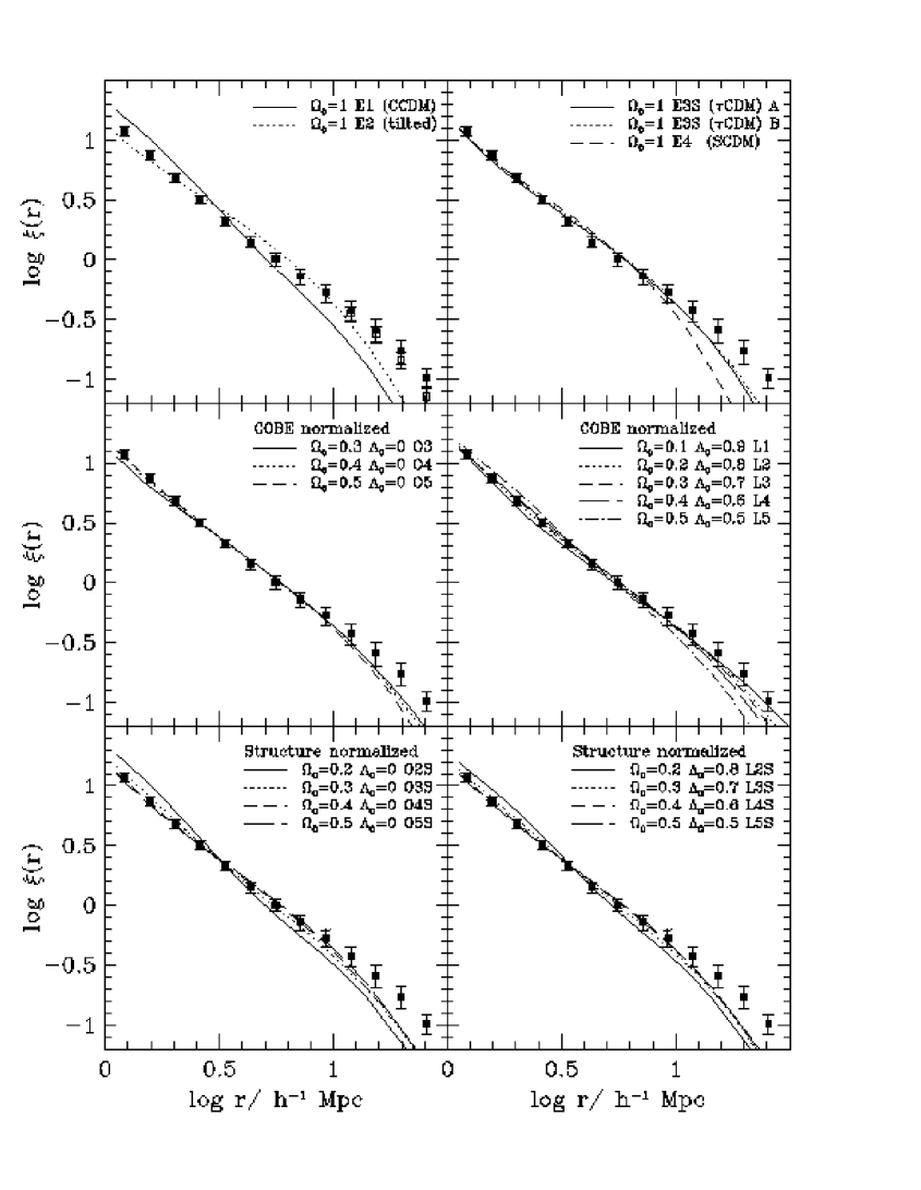
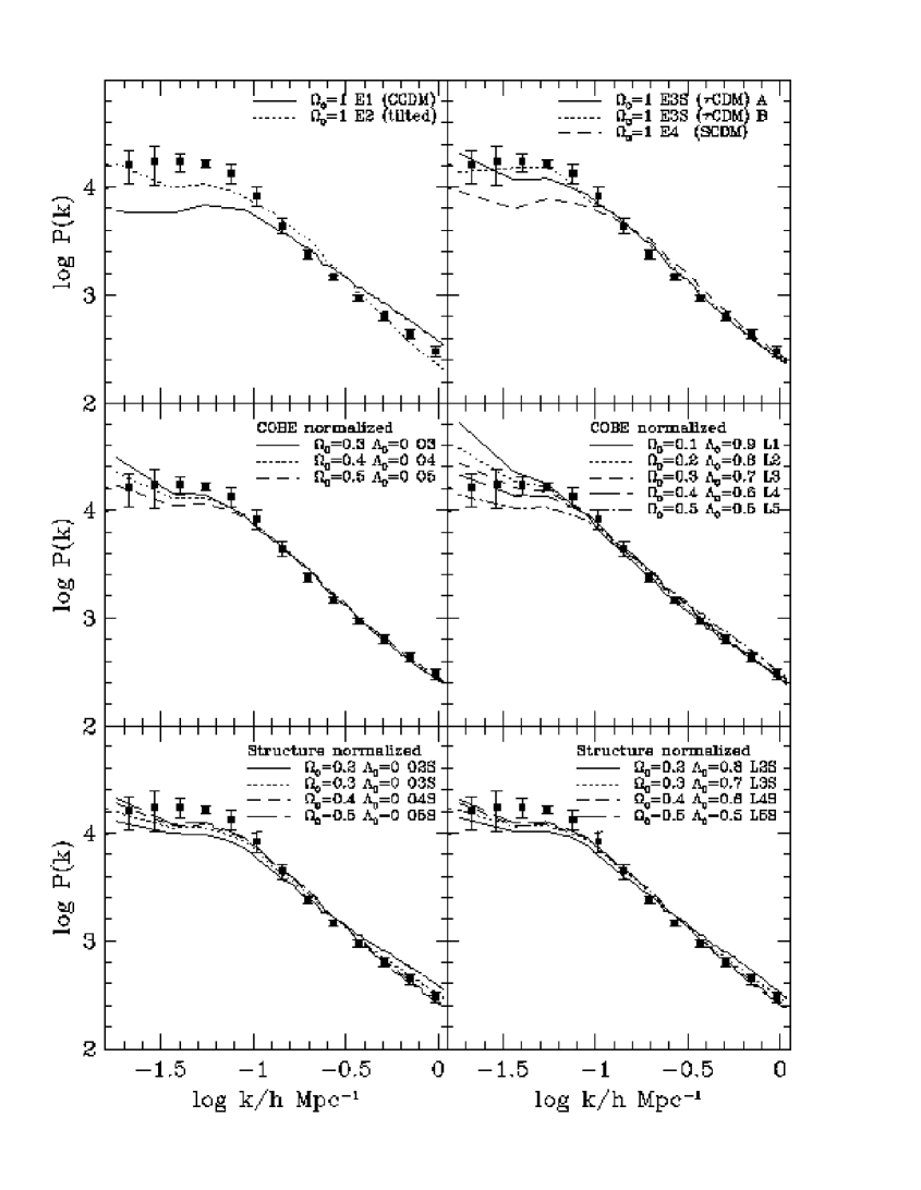
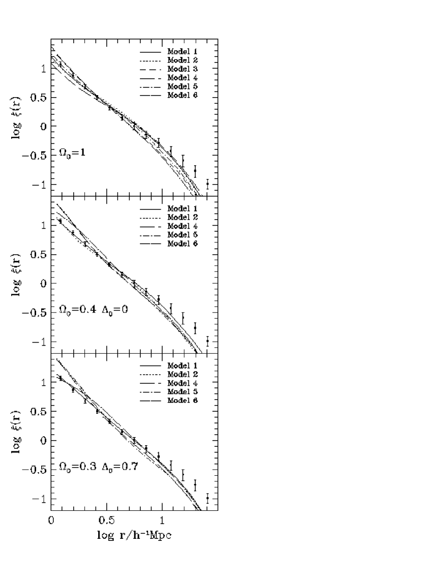
Here we define the selection probability functions, $P(\nu)$, which define each of our biasing algorithms. The resulting biased galaxy correlation functions, $\xi(r)$, and power spectra, $P(k)$, are shown in Figs. 1, 2, and 3 and discussed below. The biasing algorithm that we apply to all of the cosmological models is model 1; the other biasing models are used only to create additional mock catalogues for the O4S, L3S, and E3S simulations.

Figure 1: The galaxy correlation functions, $\xi(r)$, for each of our cosmological models when biased using bias model 1. Each of the lines corresponds to a different cosmological model as indicated on the legend. The solid data points are the same on each panel and are an estimate of the galaxy correlation function from the APM survey (Baugh 1996). The open data points, shown on the first panel, show an alternative estimate of the APM correlation function obtained by Fourier transforming the Baugh & Efstathiou (1993) estimate of the APM power spectrum.

Figure 2: The galaxy power spectrum, $P(k)$, for each of our cosmological models when biased using bias model 1. Each of the lines corresponds to a different cosmological model as indicated on the legend. The data points are the same on each panel and are an estimate of the galaxy power spectrum from the APM survey (Baugh & Efstathiou 1993).

Figure 3: For three selected, structure normalized cosmological models (E3S,O4S and L3S), we show the galaxy correlation functions that result from each of the bias models. Note that both of the $\Omega_{0}<1$ models require anti-bias and therefore cannot be biased using the peaks bias model 3. The line types corresponding to each of the bias models are indicated on the legend. The data points again show the estimate of the galaxy correlation function from the APM survey.

1. This model bases the selection probability on the value of the smoothed initial density. The initial density field is smoothed with a Gaussian of width $R_{\rm S}=3h^{-1}\,{\rm Mpc}$ (in $\exp(-r^{2}/2R_{S}^{2})$) to define a smoothed density field $\rho_{\rm S}({\bf r})$ at the initial particle position. A dimensionless variable $\nu$ is defined as $\nu({\bf r})~{}=~{}\delta_{\rm S}({\bf r})/\sigma_{\rm S}$, where the density perturbation $\delta_{\rm S}({\bf r})~{}=~{}(\rho_{\rm S}({\bf r})~{}-~{}\bar{\rho})~{}/~{}\bar{\rho}$ , and $\sigma^{2}_{\rm S}=\langle|\delta_{\rm S}|^{2}\rangle$. We then adopt

   $$P(\nu)\propto\cases{\exp(\alpha\nu+\beta\nu^{3/2})&if $\nu\geq 0$\cr\exp(\alpha\nu)&if $\nu\leq 0$\cr},$$ (3.4)

   as the selection probability. The model has two free parameters $\alpha$ and $\beta$. This choice of functional form is essentially selected for its simplicity. Its exponential form ensures that the probability cannot be negative. The dependence on $\beta$ for $\nu>0$ enables the selection probability to be enhanced ($\beta>0$) or suppressed ($\beta<0$) in the densest regions. It is this property which gives some control over the slope of the small scale correlation function. The choice of $\nu^{3/2}$ is such that the probability converges when integrated over a Gaussian distribution of $\nu$.

2. For this model the same functional form (equation 3.4) is used to define the selection probability, but this time the variable $\nu$ is defined in terms of the smoothed final density field around each particle. Again, a Gaussian smoothing with $R_{\rm S}=3h^{-1}\,{\rm Mpc}$ is adopted.

3. This is the standard high peaks model of Bardeen et al. ([1986]). Their results are used to predict the number of peaks of amplitude $\nu>\nu_{\rm p}$ defined on the scale of a galaxy as a function of the density smoothed on a larger scale that is resolvable in our simulation. In this case we choose the larger scale to be defined by applying a sharp cutoff to the power at a wavelength $\lambda\mathrel{\hbox{\hbox to0.0pt{\hbox{\lower 4.0pt\hbox{$\sim$}}\hss}\hbox{$<$}}}4h^{-1}\,{\rm Mpc}$, which is quite well resolved in the initial conditions of the simulation. We define the galaxy mass scale by a Gaussian smoothing with $R_{\rm S}=0.54h^{-1}\,{\rm Mpc}$ as adopted by White et al. ([1987]). Here the model parameter is $\nu_{\rm p}$. An unavoidable property of assuming that galaxies form in peaks of the density field is that they are more clustered than the mass distribution ($b>1$). Thus this method cannot be applied in cases where an anti-bias is required.

4. In this model a sharp cut-off is applied to the final smoothed density field, so that galaxies are entirely prohibited from forming in very underdense regions, but have an equal chance of forming wherever the overdensity rises above a certain threshold, $\rho_{\rm T}$. Thus

   $$P(\nu)\propto\cases{1&if $\rho({\bf r})\geq\rho_{\rm T}$\cr 0&if $\rho({\bf r})\leq\rho_{\rm T}$\cr}.$$ (3.5)

   This is the case if a bias greater than unity is required. For an anti-bias, the conditions are reversed and galaxies are prohibited from forming in the very densest regions. Note that this prescription for producing anti-bias seems quite unphysical, as it implies that the highest mass density regions have no galaxies at all.

5. As in model 2 the selection probability is defined in terms of the smoothed final density, but this time the functional form adopted is a power law,

   $$P(\nu)\propto\nu^{\alpha}.$$ (3.6)

   Here a positive value of the parameter, $\alpha$, will induce a bias ($b>1$) and a negative value an anti-bias ($b<1$). The bias inferred by Cen & Ostriker ([1993]) from their hydrodynamic cosmological simulations has roughly this form, with $\alpha\approx 1.5$.

6. This algorithm is a variation of model 2 and again uses the formula (3.4), but with a different definition of the overdensity parameter $\nu$. Instead of smoothing on a fixed scale of $3h^{-1}\,{\rm Mpc}$, the distribution was adaptively smoothed by setting the density at the position of each particle, $\rho\propto 1/r^{3}_{10}$, where $r_{10}$ is the distance to the 10th nearest neighbour of that particle.

The various galaxy correlation functions and power spectra resulting from applying biasing model 1 to each of our cosmological simulations are shown in Fig. 1 and Fig. 2 respectively. The solid data points show the estimates of the galaxy correlation function, $\xi(r)$, ([1996]) and power spectrum, $P(k)$, ([1993]) of APM galaxies, scaled in amplitude to match the updated estimate of $\sigma^{\rm gal}_{8}=0.96$ for the APM survey ([1996]). The data points plotted as open symbols on the top left panel of Fig. 1 show the APM correlation function as estimated from the Fourier transform of the estimated APM power spectrum. There is a slight difference between this and the direct estimate at large separations, which arises because both $\xi(r)$ and $P(k)$ are estimated using non-linear inversions of the measured angular correlation function. The difference is an indication of one of the systematic errors involved in estimating $\xi(r)$ on large scales.

In general the two parameter biasing model is successful in matching both the amplitude and the shape of the galaxy correlation function on scales of $1$–$10h^{-1}\,{\rm Mpc}$, as can clearly be seen in Fig. 1. For a few cases, such as E1, O2S, and L2S, which have high values of $\sigma^{\rm mass}_{8}$ and consequently steep non-linear mass correlation functions, the bias model cannot reduce the slope of the correlation function enough to accurately match the observed value. The behaviour of the correlation functions on large scales reflects each model’s value of the power spectrum shape parameter $\Gamma$. The APM data, if fitted with a $\Gamma$-model, prefer $\Gamma=0.15$–$0.2$ (e.g. [1990]), so even our structure normalized, $\Gamma=0.25$ models fall short of the amount of large-scale power evident in the APM correlation function. This short-fall is also exaggerated by a statistical fluctuation in our simulation initial conditions. As can be seen in the top-righthand panel of Fig. 2, the first realization (A) of model E3S has less power on scales $0.03\mathrel{\hbox{\hbox to0.0pt{\hbox{\lower 4.0pt\hbox{$\sim$}}\hss}\hbox{$<$}}}k\mathrel{\hbox{\hbox to0.0pt{\hbox{\lower 4.0pt\hbox{$\sim$}}\hss}\hbox{$<$}}}0.06\,h$Mpc^-1 than the second realization (B) of the same model. This downward fluctuation in the power is present in all the other cosmological models, since all the initial density fields were generated from the same basic Gaussian random field but with expected mean amplitudes rescaled according to the model power spectrum. We also note that the longest wavelength modes, with $k=0.018\,h$Mpc^-1, are noisy because of the small number of such modes contained in the simulation box. The comparison of model and APM galaxy power spectra on small scales (high $k$) is in accord with the small scale behaviour of the correlation functions.

The manner in which the galaxy clustering statistics vary with the form of the biasing is illustrated in Fig. 3. The 1-parameter bias models (models 3, 4 and 5) do not have the flexibility to control both the amplitude and slope of the galaxy correlation function. Thus, in general, these models do not match the APM galaxy correlation function over a wide range of scales. In particular, the galaxy correlation functions of the three models selected for Fig. 3 are steeper than the correlation function of APM galaxies, reflecting the steepness of the underlying mass correlation functions. The $3h^{-1}\,{\rm Mpc}$ filter used in bias model 2 smooths over the structure of groups and clusters in the final density field. As a result, the small-scale slope of the galaxy correlation function ends up being insensitive to the bias model parameters in this case. In model 6, on the other hand, the use of an adaptive smoothing results in better resolution on the scale of groups and clusters. In some cases this is enough to enable the required adjustments to the slope of the correlation function on small scales.

3.3.2 The asymptotic bias

In general all the biasing algorithms discussed above give rise to a bias that is scale dependent. However, since these biasing algorithms only depend on local properties of the density field, the bias should tend to a constant on large scales. Where the selection probability is a function of the initial density field, the value of this asymptotic bias can be computed analytically. The probability that a mass particle is selected as a galaxy is taken to be $P(\nu)$, where $\nu$ is the amplitude of the initial density fluctuation in units of the rms, $\sigma_{\rm s}$. The normalization of $P(\nu)$ is determined by the integral over the Gaussian distribution of initial density fluctuations,

$$\frac{1}{\sqrt{2\pi}}\int P(\nu)\,e^{-\nu^{2}/2}\,d\nu=1.$$ (3.7)

The density of galaxies selected in a region in which a large scale perturbation $\Delta$ is added will be given by

$$\rho_{\rm gal}=\bar{\rho}_{\rm gal}\,\frac{(1+\Delta)}{\sqrt{2\pi}}\int P(\nu^{\prime})\,e^{-\nu^{2}/2}\,d\nu,$$ (3.8)

where $\nu^{\prime}=\nu+\Delta/\sigma_{\rm s}$. A first order series expansion of $P(\nu)$ yields

$$P(\nu^{\prime})=P(\nu)\left(1+\frac{d\ln P}{d\nu}\,\frac{\Delta}{\sigma_{\rm s}}\right).$$ (3.9)

Hence

$$\frac{\rho_{\rm gal}}{\bar{\rho}_{\rm gal}}=\frac{(1+\Delta)}{\sqrt{2\pi}}\int P(\nu)\left(1+\frac{d\ln P}{d\nu}\frac{\Delta}{\sigma_{\rm s}}\right)e^{-\nu^{2}/2}d\nu,$$ (3.10)

which simplifies to

$$\frac{\rho_{\rm gal}}{\bar{\rho}_{\rm gal}}=(1+\Delta)\left(1+\frac{\Delta}{\sqrt{2\pi}\sigma_{\rm s}}\ \int\frac{dP}{d\nu}\,e^{-\nu^{2}/2}\,d\nu\right).$$ (3.11)

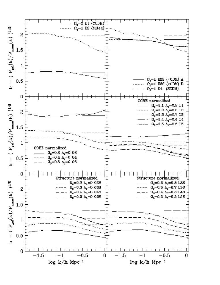
We can thus define an asymptotic bias factor, i.e. the ratio of the galaxy to the mass perturbations on large scales, as

$$b_{\rm asymp}=1+\frac{1}{\sqrt{2\pi}\sigma_{\rm s}}\int\frac{dP}{d\nu}\,e^{-\nu^{2}/2}\,d\nu.$$ (3.12)

This result is compared to the bias estimated from the simulations in Fig. 4. The figure clearly shows that the bias does indeed tend towards its asymptotic value, as calculated above, on large scales.

Figure 4: The scale-dependent bias, $b(k)=P_{\rm gal}(k)/P_{\rm mass}(k)$, for each of our cosmological models when biased using bias model 1. Each of the lines corresponds to a different cosmological model as indicated on the Figure. To the right of each panel we show the value of the expected asymptotic bias on large scales, as explained in Section 3.3.2.

4 Mock Catalogues

In the previous section we described the procedure by which we create a galaxy distribution within each simulation cube. We now describe how these are manipulated and sampled to create the mock galaxy catalogues. It should be noted that we do not attempt to mimic the imperfections that will inevitably be present in the genuine catalogues, e.g. , Galactic extinction, excluded regions around bright stars, or missing members of galaxy pairs separated by less than the minimum fibre spacing. Our goal is instead to create idealized catalogues with the expected redshift distributions and geometrical properties of the genuine surveys. We anticipate that members of the 2dF and SDSS collaborations will create a few mock catalogues that incorporate the finer details of the survey properties.

4.1 Survey geometry

Figure 5: An equal area (Mollweide) projection of the whole sky showing the regions covered by the 2dF and SDSS galaxy redshift surveys. The regions covered by the 2dF survey are indicated by the areas populated by points. These are the galaxy positions for a narrow range in redshift from one of our mock catalogues. The 2dF consists of two strips. The larger crosses the SGP while the small one runs close to the NGP. The solid curve marks the boundary of the SDSS survey, which is an ellipse centred close to the NGP. We do not include the SDSS southern strips. The grid indicates the RA and dec. coordinates.

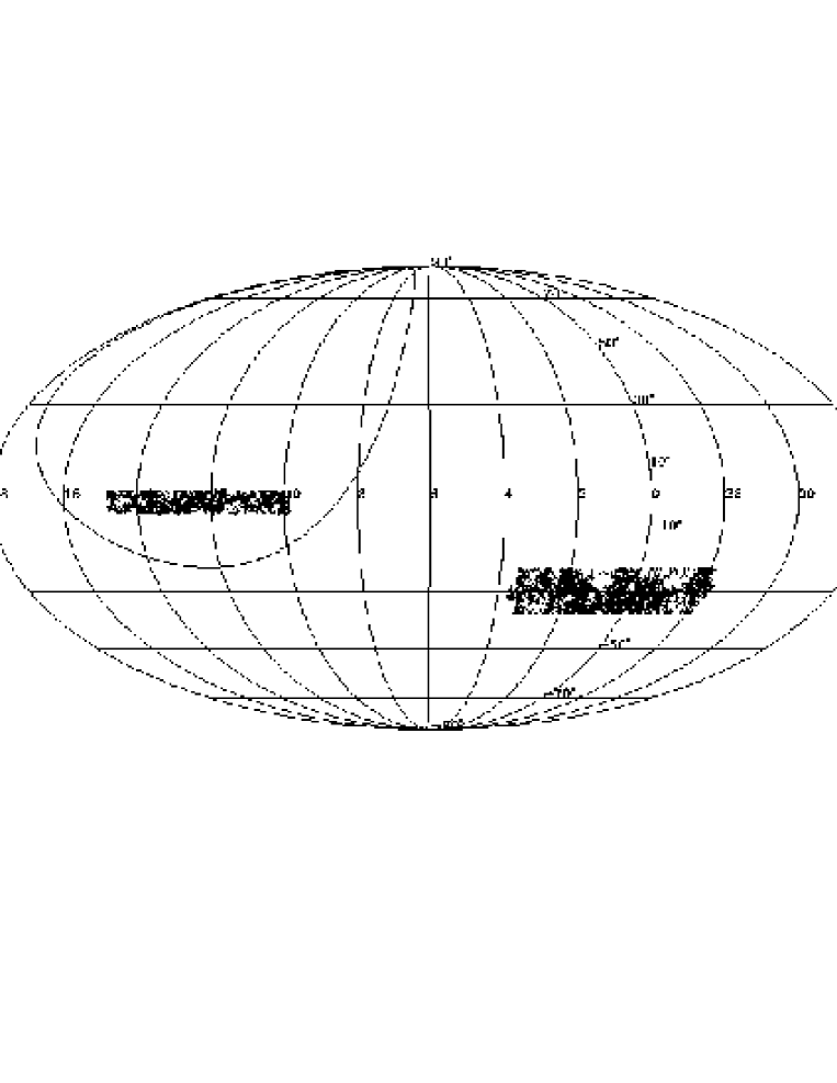
The specifications of both the 2dF and Sloan surveys may be slightly modified after evaluating the results from the current period of test observations. The areas which we have adopted are shown in Fig. 5 and defined below.

The main SDSS area is an elliptical region centred at ${\rm R.A.}=12^{\rm hr}20^{\rm m}$ $\delta=32.8^{\circ}$, close to the North Galactic Pole (NGP) and covering $3.11$ steradians. The minor axis of the ellipse spans $110^{\circ}$ and runs along a line of constant R.A. The major axis spans $130^{\circ}$. Our mock catalogues do not include the strips in the Southern Galactic Cap that will also be part of the SDSS redshift survey; larger simulation volumes are needed to model simultaneously the Northern and Southern SDSS.

The main 2dF survey consists of two broad declination strips. The larger is approximately centred on the SGP and covers the declination range $-22.5^{\circ}>\delta>-37.5^{\circ}$. This declination range breaks into three contiguous, $5^{\circ}$ wide strips, each with slightly different ranges in R.A., which from north to south are $21^{\rm hr}48^{\rm m}<{\rm R.A.}<3^{\rm hr}24^{\rm m}$, $21^{\rm hr}39.5^{\rm m}<{\rm R.A.}<3^{\rm hr}43.5^{\rm m}$ and $21^{\rm hr}49^{\rm m}<{\rm R.A.}<3^{\rm hr}29^{\rm m}$. The smaller strip in the northern galactic hemisphere covers $-7.5^{\circ}<\delta<2.5^{\circ}$ and $9^{\rm hr}50^{\rm m}<{\rm R.A.}<14^{\rm hr}50^{\rm m}$. Together they cover a solid angle of $0.51$ steradians. There is considerable overlap between the northern slice and the area covered by the SDSS.

4.2 The radial selection function

The galaxies of the 2dF survey are selected from the APM galaxy survey and will be complete to an extinction corrected apparent magnitude of $B_{\rm J}<19.45$. The SDSS will have galaxies selected from its own multi-band digital photometry. The primary selection will be made in the Gunn-$r$ band, and it will include a surface brightness threshold to ensure that an adequate fraction of the galaxy light goes down a $3^{\prime\prime}$ fibre (see [1995] for details). For simplicity, and because our goal is merely to match the geometry and depth of the two surveys, we make our selection for both catalogues in the $B_{\rm J}$ band. For the SDSS we adopt a magnitude limit of $B_{\rm J}<18.9$ so as to approximately reproduce the SDSS target of 900,000 galaxies in the survey area. A mock catalogue from a $(600h^{-1}\,{\rm Mpc})^{3}$ $N$-body simulation that mimics the SDSS selection function in greater detail will be presented elsewhere (Gott et al., in preparation; see also [1995]). In addition to its primary galaxy sample, the SDSS will target a set of $\sim 100,000$ luminous red elliptical galaxies, to create a deep, sparse sample that is approximately volume-limited to $z\sim 0.4$. Similarly, the 2dF programme includes a deep extension to $R\sim 21$ which will contain $\sim 10000$ galaxies. We do not attempt to model these samples because their median depths are larger than our simulation cubes.

In order to compute the radial selection functions of the surveys, we adopt a Schechter function description of the $B_{\rm J}$ band luminosity function,

$$\frac{d\phi(L)}{dL}\,dL=\phi_{\star}\,(L/L_{\star})^{{\alpha_{\star}}}\,\exp(-L/L_{\star})\,dL/L_{\star},$$ (4.13)

with absolute magnitude $M_{B_{\rm J}}=M^{\odot}_{B_{\rm J}}-2.5\log_{10}(L/L_{\odot})$. We relate the apparent magnitude $B_{J}$ of a galaxy at redshift $z$ to the corresponding absolute magnitude $M_{B_{\rm J}}$ at redshift $z=0$ using

$$B_{\rm J}\negthinspace=\negthinspace{\rm e}+{\rm k}+5\log_{10}(d_{L}/h^{-1}\,{\rm Mpc})+25+(M_{B_{\rm J}}-5\log_{10}h).$$ (4.14)

Here $d_{L}$ is the luminosity distance to redshift $z$ in the appropriate cosmological model. The term “k” denotes the so called k-correction, which arises from the Doppler shift to the wavelength of the galaxy’s spectral energy distribution when viewed in the observer’s frame. The term “e” describes the effect of luminosity evolution in the galaxy as a result of a combination of passive evolution of the stellar populations and star formation. This model therefore allows for luminosity evolution, but not for any change in the shape of the galaxy luminosity function, which might occur as a result of galaxy merging or luminosity dependent evolution.

Even over the relatively limited range of apparent magnitudes covered by the APM survey, the galaxy number counts are a significantly steeper function of apparent magnitude than is predicted by non-evolving models ([1990b]). In contrast The K-band galaxy counts have shown no evidence for such a steep slope [1997], but recently Phillips & Turner (1998) have used a compilation of survey data to argue that at the brightest magnitudes the K-band slope is as steep as that seen in the B-band. Unless we live in a very large underdense region or there exists some as yet unidentified systematic error in the bright galaxy counts, some form of rapid galaxy evolution is necessary. The counts can be reproduced by a model with strong luminosity evolution such as can be accommodated in eqn. (4.2), but at somewhat fainter magnitudes than those covered by the SDSS and 2dF surveys such a model predicts a tail of high redshift galaxies that is not seen in deep spectroscopic galaxy samples (e.g. [1990]). Thus, a more complicated form of evolution is required, either one in which different galaxies evolve at different rates or one in which galaxies merge so that the number of galaxies is not conserved. The new redshift surveys themselves will give important information on evolution of the galaxy luminosity function. However, for the purposes of quantifying large structure this is not a problem provided that the selection function can be accurately determined. We have therefore adopted a simple model that produces a selection function with similar depth to that which we expect the surveys to have.

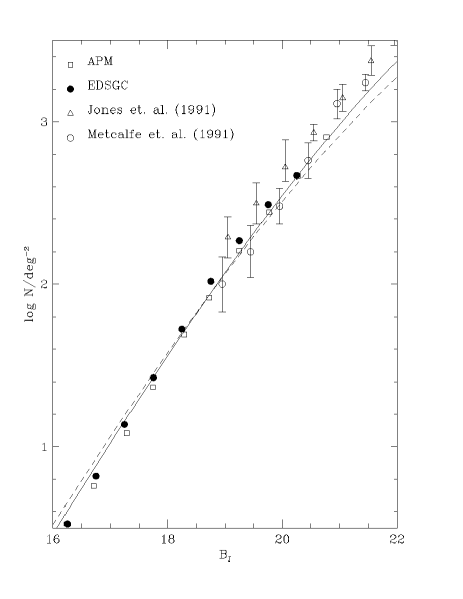
In our standard model we adopt the parameters found by Loveday et al. ([1992]) for the APM-Stromlo bright galaxy survey, $M^{\star}_{B_{\rm J}}-5\log_{10}h=-19.5$, $\alpha_{\star}=-0.97$ and $\phi_{\star}=1.4\times 10^{-2}h^{3}{\rm Mpc}^{-3}$. We also set ${\rm k}+{\rm e}=0$, i.e. we assume that strong luminosity evolution occurs which cancels the k-correction. While this cancellation seems coincidental, Fig. 6 shows that this simple choice gives reasonable agreement with the observed galaxy number counts at $B_{J}\approx 19.5$ and so will produce mock galaxy catalogues with approximately the number of galaxies expected in the 2dF survey.

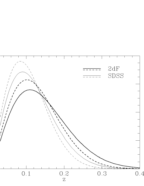
As a variation, we have also produced a selection of mock catalogues in which the artificial assumption that ${\rm k}+{\rm e}=0$ has been dropped. For these we use the evolution law ${\rm k}+{\rm e}=2.5\log_{10}(1+z)$, which corresponds to weaker luminosity evolution than in our standard model. To compensate for this we increase the value of $\phi_{\star}$ by 24% to $1.73\times 10^{-2}h^{3}{\rm Mpc}^{-3}$ to keep the total number of galaxies in the survey approximately the same as in our standard model. This model’s galaxy counts and redshift distributions (for the case of $\Omega_{0}=1$) are shown by the dashed lines in Figs. 6 and 7.

Figure 6: Galaxy number counts in our two evolution models compared with observational data. Over this range of magnitudes, the counts are weakly dependent on cosmology and are plotted here for $\Omega_{0}=1$. The solid line corresponds to our standard model in which luminosity evolution cancels the k-corrections. The dashed line corresponds to the less extreme model in which k-corrections are larger than the luminosity evolution. The data points are taken from Maddox et al. (1990b) (APM), Heydon-Dumbleton, Collins & MacGillivray (1989) (EDSGC), Jones et al. (1991) and Metcalfe et al. (1991).

Figure 7: The model galaxy redshift distributions. These distributions are weakly dependent on cosmology and are plotted here for $\Omega_{0}=1$. The heavy curves, peaking at the higher redshifts, correspond to the magnitude limit of $B_{\rm J}<19.45$ of the 2dF survey and light lines to the $B_{\rm J}<18.9$ of the SDSS. As in Fig. 6, the solid curves are for our standard selection function and the dashed curves for the alternative model with weaker luminosity evolution. The median redshifts are $z_{\rm m}=0.13$ and $0.12$ for the 2dF catalogues and $z=0.11$ and $0.10$ for the SDSS catalogues.

4.3 Survey construction

The task of generating a mock galaxy catalogue now consists of two steps: choose the location of the observer, and select galaxies subject to the geometrical constraints and radial selection function specified above.

To aid in the comparison between the different cosmological models, we choose to place the observer at the same position in each of the galaxy catalogues. The observer’s position was essentially chosen at random, although we did apply the weak constraint that the velocity dispersion of particles within $5h^{-1}\,{\rm Mpc}$ of the observer should be less than $350{\rm km\,s^{-1}}$ in the $\Omega=1$ model, in order to avoid observers placed in rich galaxy clusters. This constraint was only directly applied in model E3S, but by virtue of the fact that all our simulations have the same phases it is effectively satisfied in all the structure normalized models. However, for the COBE normalized simulations that have $\sigma_{8}$ greater than that required to match the observed abundance of rich clusters, the galaxy velocity dispersion is typically higher, and the constraint may be violated. For most analyses of the 2dF and Sloan surveys the choice of the observer should not be important, as the volumes of the surveys are large compared to the local region whose properties are constrained by the choice of observer.

Having chosen the observer’s location, we replicate the periodic cube of the $N$-body simulation around the observer to reach a depth of $z=0.5$. We choose the same position for the observer in both the 2dF and SDSS surveys, but the observer’s orientation was not chosen consistently between the two surveys. We then loop over all the galaxies within the geometrical boundaries of the survey. From the model luminosity function and cosmological model we compute the expected mean number density $\bar{n}_{\rm s}(r)$ of galaxies brighter than the survey magnitude limit at the distance $r$ of each of these galaxies. We then select the galaxy zero, one or more times according to a Poisson distribution with mean $\bar{n}_{\rm s}(r)/\bar{n}_{\rm g}$, where $\bar{n}_{\rm g}$ is the mean galaxy number density in the biased galaxy distribution described in Section 3.3. In this process approximately 1% of the galaxies are selected more than once and appear with identical positions and velocities in the mock catalogue. This double sampling essentially never occurs at $z>0.02$, where the selection function drops to a space density less than $n_{\rm g}$. For each selected galaxy we generate an apparent $B_{\rm J}$ magnitude consistent with the selection function, and also a value of $z_{\rm max}$, defined as the redshift corresponding to the maximum distance at which the younger counterpart of the galaxy would still be brighter than the survey apparent magnitude limit. In computing this redshift we include the effect of both the k-correction and evolution on the galaxy’s luminosity. As our idealized models assume that galaxy mergers do not take place this definition of $z_{\rm max}$ makes it easy to contruct volume limited catalogues in which the mean galaxy density is independent of redshift. For the genuine surveys removing the effect of evolution from the radial dependence of the galaxy density field will be more problematic as evolutionary corrections for each galaxy will be uncertain and over the limited redshift range probed by these surveys galaxy mergers may also play a small role. In our catalogues we record the galaxy redshift, its angular coordinates, the redshift it would have if it had no peculiar velocity, its apparent $B_{\rm J}$ magnitude, and $z_{\rm max}$. We also record an index which can be used to identify the particle to which it corresponded in the original $N$-body simulation.

4.4 Adding long wavelength power

For a subset of simulations we have applied a technique which allows the spectrum of density fluctuations present in the final galaxy catalogues to be extended to wavelengths longer than those included in the original $N$-body simulation. This method, dubbed the Mode Adding Procedure (MAP), was proposed by Tormen & Bertschinger ([1996]) and discussed further by Cole ([1997]). Essentially, one uses the Zel’dovich approximation with a change of sign to remove from the $N$-body particle distribution the displacements caused by the longest wavelength modes in the original simulation. This can be done accurately if these modes are still in the linear regime. One then generates a new large scale density field in a much larger box, which samples this same region of ${\bf k}$-space more finely. Displacements are computed by the Zel’dovich approximation from this new field and used to perturb both the original simulation cube and the adjacent replicas. The displacements applied to each of the replicas differ, as the new large scale density field is not periodic on the scale of the original simulation cube. We choose to remove the inner $5^{3}$ modes from the original simulations and generate the large scale density field in a box with edge $7$ times that of the original simulation ($N_{\rm S}=2$ and $L/S=7$ in the notation of Cole [1997]).

As pointed out by Cole ([1997]), it is important that the biasing algorithm takes account of the effect of the added long wavelength power. This is most easily done for algorithms such as model 1, which are a function of the initial linear density field. One simply replaces the original linear density field by a new one constructed by removing the original long wavelength power and adding the new large scale density field. It is more complicated to correctly apply a biasing algorithm that is a function of the final density field, because the final density field is non-linear, and its short wavelength modes are coupled to the linear long wavelength modes. With this in mind, we applied the MAP only in combination with our bias model 1. In order to keep computer storage requirements within reasonable bounds, it is necessary to combine into a single program the application of the MAP, the biasing prescription, and the survey selection criteria.

4.5 Inventory

For each of the cosmological simulations listed in Table 1 (21, including the second realization of model E3S), we have created mock SDSS and 2dF surveys using bias model 1 and the standard selection function, in which the evolution and k-corrections cancel. The MAP was not used to add long wavelength power to these catalogues. For four structure-normalized cosmological simulations — the open $\Omega_{0}=0.4$ model (O4S), the flat $\Omega_{0}=0.3$ (L3S), and the two realizations of the Einstein-de Sitter model (E3S) — we constructed a number of variants: changing the bias model to models 2, 3, 4, 5, and 6; without bias; using the variation of the selection function described in Section 4.2, in which luminosity evolution is weaker than the k-corrections; and using bias model 1 with long wavelength power added using the MAP.

5 Illustrations

We now compare and contrast the visual properties of the galaxy distributions in each of the mock catalogues using a series of redshift space wedge diagrams.

Figure 8: Redshift space slices showing galaxy positions from a variety of the mock 2dF galaxy catalogues. Each wedge shows a strip $90^{\circ}$ wide in R.A. and $3^{\circ}$ thick in declination, extending to $z=0.3$. Each of the six models shown is normalized by the present abundance of galaxy clusters and biased using model 1 (see Section 3.3). The inset square panels illustrate the effect of bias by showing the real space particle and galaxy distributions in a $100\times 100\times 20h^{-1}\,{\rm Mpc}$ slab. The top panels show $\Omega_{0}=1$ models: E3S ($\tau$CDM) on the left and E4 (SCDM) on the right. Below these are the open and flat $\Omega_{0}=0.5$ models, O5S and L5S, and, at the bottom, the open and flat $\Omega_{0}=0.2$ models, O2S and L2S.

Figure 9: Redshift space slices from the cluster normalized mock SDSS catalogues. The correspondence between model and panel is the same as for Fig. 8. The slices are $130^{\circ}$ wide by $6^{\circ}$ thick and extend to $z=0.2$. The qualitative differences between the structure visible in these slices and in the corresponding 2dF slices of Fig. 8 are due to the choice of slice thickness and depth rather than any intrinsic difference in the 2dF and SDSS selection functions.

Figure 10: Redshift space slices from the mock 2dF catalogues for the tilted CDM model E2 (top left) and the open COBE normalized models, O5, O4 and O3. The corresponding value of $\Omega_{0}$ and the normalization $\sigma_{8}$ are indicated on each panel. The geometry of the slices and inset plots of the real space mass and galaxy distributions is the same as in Fig. 8.

Figure 11: Redshift space slices from the mock SDSS catalogues for the same models as Fig. 10, the tilted CDM model E2 and the open COBE normalized models, O5, O4 and O3. The geometry of the slices is the same as in Fig. 9.

Figure 12: Redshift space slices from the mock 2dF catalogues for the flat COBE normalized models, E1 (CCDM), L1, L2, L3, L4 and L5. The corresponding values of $\Omega_{0}$, $\Lambda_{0}$ and the normalization $\sigma_{8}$ are indicated on each panel. The geometry of the slices and inset plots of the real space mass and galaxy distributions are the same as in Fig. 8.

Figure 13: Redshift space slices from the mock SDSS catalogues for the same models as Fig. 12, the flat COBE normalized models, E1 (CCDM), L1, L2, L3, L4 and L5. The geometry of the slices are the same as in Fig. 9.

Figure 14: Redshift space slices from the mock 2dF catalogues showing the effect of varying the choice of biasing algorithm. Each slice was constructed from the same cosmological model E3S ($\tau$CDM), but with a variety of biasing algorithms as indicated on each panel. The panel at the bottom right shows the effect of using the MAP in conjunction with bias model 1 to add long wavelength power to the mock catalogue. The geometry of the slices and inset plots of the real space mass and galaxy distributions are the same as in Fig. 8.

Figure 15: A comparison of the galaxy distribution in redshift space (upper panel) and real space (lower panel) for a $2^{\circ}$ thick slice from a SDSS mock catalogue constructed from model E3S ($\tau$CDM).

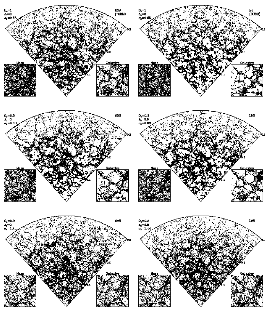
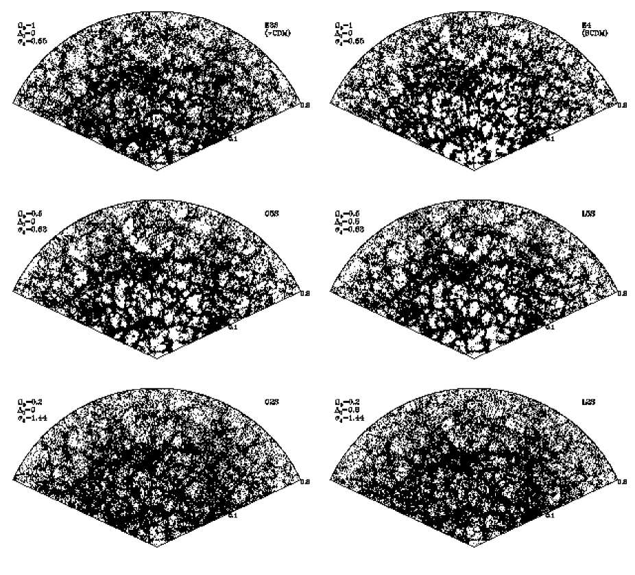
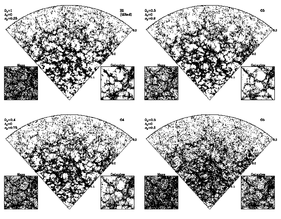
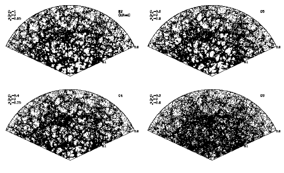
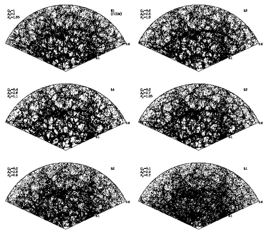
Figs. 8 and 9 show the galaxy distribution in redshift space slices extracted from the mock 2dF and SDSS catalogues constructed from the cluster-normalized $N$-body simulations. Each of the catalogues was biased using model 1 of Section 3.3. The 2dF slices (Fig. 8) are $90^{\circ}$ wide in R.A., $3^{\circ}$ thick in declination and plotted out to a redshift of $z=0.3$. By contrast, the SDSS slices (Fig. 9), which are $130^{\circ}$ wide (corresponding to the full length of the long axis of the SDSS ellipse) are $6^{\circ}$ thick but plotted only to $z=0.2$. A visual inspection reveals that the structure in all six models looks remarkably similar. This is essentially a reflection of the facts that all the simulations were started with the same phases and that the observer is alway located at the same position. Also, because these models are designed to produce similar abundances of rich galaxy clusters, the strength of the “fingers-of-god” effect is also similar. The 1-dimensional galaxy velocity dispersions in all the cluster-normalized models is in the range $440-465{\rm km\,s^{-1}}-$. The visible effects on the galaxy distribution that result from varying $\Omega_{0}$, $\Lambda_{0}$, and the amount of large scale power ($\Gamma$) are quite subtle. Of the two $\Omega_{0}=1$ models, E3S ($\tau$CDM) has more large scale power than E4 (SCDM). A manifestation of this is that structure in E3S ($\tau$CDM) appears more connected and less choppy than that of E4 (SCDM). The changes that occur when $\Omega_{0}$ is varied are related to the strength of galaxy biasing. For models that are normalized to produce the observed abundance of rich clusters, the amplitude of mass fluctuations, $\sigma_{8}$, increases as $\Omega_{0}$ is decreased. Thus, the $\Omega_{0}=1$ models require a strong bias, the $\Omega_{0}=0.5$ models a weak bias, and the $\Omega_{0}=0.2$ models an anti-bias. The effect of this can be seen most clearly in the inset square panels of Fig. 8. These show, in real space, a $100\times 100\times 20h^{-1}\,{\rm Mpc}$ slab of the mass and corresponding galaxy distribution, both sampled to the same density of $\bar{n}_{\rm g}\approx 0.05h^{3}{\rm Mpc}^{-3}$. In the $\Omega_{0}\geq 0.5$ models, the biasing algorithm clearly has the effect of mapping underdense regions in the mass distribution to completely empty voids in the galaxy distribution. In the anti-biased, $\Omega_{0}=0.2$ models, galaxies continue to trace the mass in the underdense regions. Finally, comparison of the open and flat models indicates that the value of the cosmological constant, $\Lambda_{0}$, has virtually no detectable effect on the galaxy distribution.

Figs. 10 and 11 show redshift space slices with the same geometry as those of Figs. 8 and 9. The top left hand panels in each figure show the tilted $\Omega_{0}=1$ model, E2, which by virtue of the tilt is both cluster and COBE normalized. These distributions should be compared with those in the upper panels of Figs. 8 and 9, which show corresponding slices for our other two cluster normalized, $\Omega_{0}=1$ models. The tilted (E2) model appears intermediate in character between the $\tau$CDM (E3S) and SCDM (E4) models. This is consistent with the relative amounts of power on scales of $50$-$100h^{-1}\,{\rm Mpc}$ in these models. The tilt of $n\approx 0.8$ with $\Gamma\approx 0.45$ produces more power on these scales than SCDM with $n=1$ and $\Gamma=0.5$, but less than $\tau$CDM with $n=1$ and $\Gamma=0.25$. The remaining three panels in Figs. 10 and 11 are for the open ($\Lambda_{0}=0$) COBE normalized models. In this sequence, as $\Omega_{0}$ is decreased $\sigma_{8}$ decreases, the bias increases, and $\Gamma$ decreases. The most visible effect comes from the variation of $\sigma_{8}$. There is a clear trend such that the mass distribution looks more evolved, with more crisply defined filaments and voids, as $\sigma_{8}$ is increased. This trend is also visible in the galaxy distribution, but here the bias partially compensates for the changing $\sigma_{8}$, and the relationship appears weaker. On small scales the effect of the random velocities within galaxy clusters is just discernible. The “fingers-of-god” are largest in the $\Omega_{0}=0.5$ in which the galaxies have a mean 1-dimensional velocity dispersion of $485{\rm km\,s^{-1}}-$ compared to only $225{\rm km\,s^{-1}}-$ in the $\Omega_{0}=0.3$

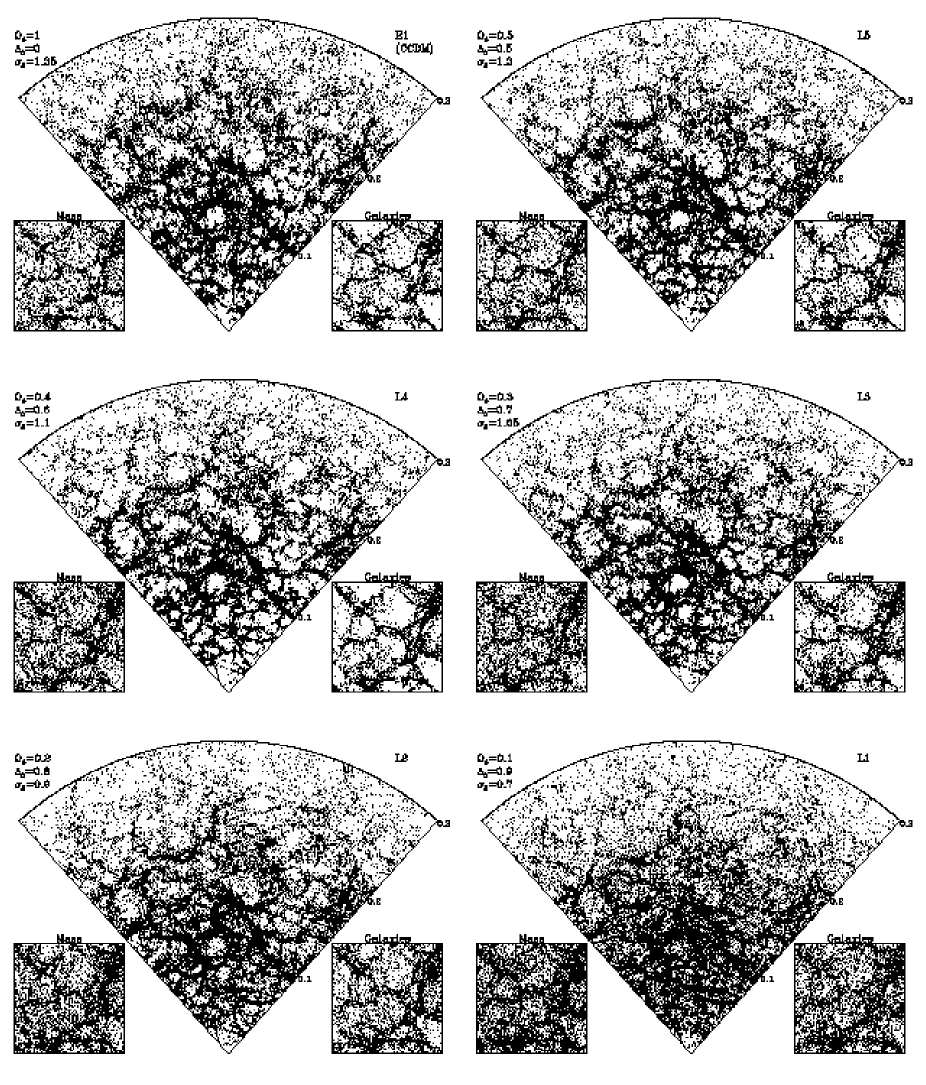
Figs. 12 and 13 show 2dF and SDSS redshift space slices for the set of COBE normalized, flat ($\Omega_{0}+\Lambda_{0}=1$) models. For this sequence of models, $\sigma_{8}$ decreases weakly as $\Omega_{0}$ decreases. Thus we see a weaker version of the same trend we noted in the open COBE normalized models. The higher $\Omega_{0}$ models have a more evolved density distribution with more sharply defined voids and filaments. Also there is a similar trend in the galaxy velocity dispersion and the resulting “finger-of-god” features. The 1-dimensional velocity dispersion is $200{\rm km\,s^{-1}}-$ for $\Omega_{0}=0.1$ and climbs to $665{\rm km\,s^{-1}}-$ for $\Omega_{0}=0.5$. The ‘fingers-of-god” are extremely pronounced in the $\Omega_{0}=1$ model which has a 1-dimensional velocity dispersion of $890{\rm km\,s^{-1}}-$.

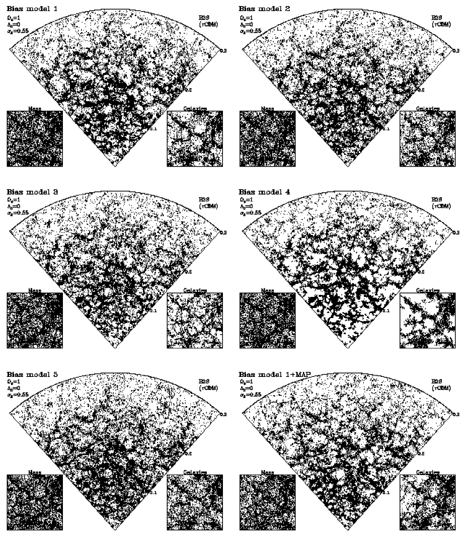
Fig. 14 shows 2dF redshift space slices illustrating the effect of varying the choice of biasing algorithm. Each slice was constructed from the same cosmological model E3S ($\tau$CDM), but with a variety of biasing algorithms as indicated on each panel. The correlation functions of each of these galaxy distributions, shown in Fig. 3, are quite similar. Despite this some of the distributions are visually quite distinct. The most striking feature is variation in the size and number of voids. The voids are largest and most numerous in bias model 4 as a result of its sharp density threshold. The models in which the bias function is a more gradual function of density, such as the power law case of model 5, have far fewer voids. The panel at the bottom right shows the effect of using the MAP in conjunction with bias model 1 to add long wavelength power to the mock catalogue. The distortion of the small scale galaxy distribution is small as the perturbations are of very long wavelength, but there effect on measurements of large scale power can be appreciable.

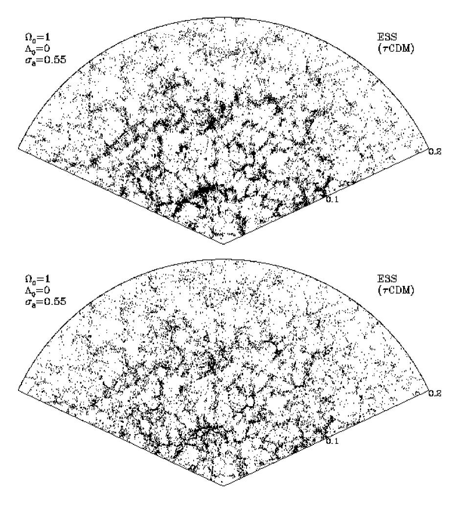
Fig. 15 contrasts the galaxy distribution in redshift space (upper panel) with what would be observed if true distances rather than redshifts were measurable (lower panel). The model that has been plotted here is the E3S ($\tau$CDM) model with galaxies selected using bias model 1. The thickness of the slice is just $2^{\circ}$.

6 Limitations

We plan to use the mock catalogues presented in this paper to help in the important task of testing and calibrating the algorithms and statistics that will be applied to the analysis of the 2dF and SDSS redshift surveys. We hope that they will be similarly useful to other researchers. However, it is important to be aware of the limitations of this compilation of mock catalogues.

1. The mock catalogues are idealized and do not suffer from some problems which, at some level, are inevitable in the genuine surveys. These include systematic errors in the photometry used to select the target galaxies, cosmetic defects such as regions cut out around bright foreground stars, failure to measure redshifts for 100% of the target galaxies, redshift measurement errors, and the residual effects of extinction by foreground dust.

2. The model selection functions are simplistic and do not allow for the effects of galaxy mergers. It will only become possible to adequately constrain evolution models that incorporate galaxy merging once the joint apparent magnitude-redshift distributions are accurately measured from the surveys themselves. Furthermore, we have not attempted to mimic the details of the SDSS target selection criteria, although we expect that the selection function of the SDSS will not differ substantially from that implied by the $B_{\rm J}$-magnitude limited criterion that we have used.

3. Evolution of clustering over the redshift range of the surveys is ignored – each of our mock catalogues is constructed from a single output time from the $N$-body simulations. Clustering evolution is probably very weak over the depth of the SDSS and 2dF surveys but it may not be negligible for deeper surveys and will be important for some applications (see, e.g. [1998]).

4. The $N$-body simulations solve the equations describing Newtonian gravity and therefore explicitly ignore space curvature across the simulation box. One consequence of this is that in the open models we are forced to use $4\pi r_{\rm c}^{2}dr_{\rm c}$, where $r_{c}$ is the comoving distance to redshift $z$, as the volume element rather than the correct relativistic expression. However for the depth of the present surveys this is a very small effect.

5. The simulations have limited mass and force resolution. The spatial resolution in the initial conditions is limited to scales greater than the mean particle separation of $1.8h^{-1}\,{\rm Mpc}$. However, the power on these scales in the final configuration is dominated by non-linear transfer from large scales. Thus, the range of reliability of the estimated correlation functions and power spectra is determined by the force resolution, $\epsilon=90h^{-1}\,{\rm kpc}$ (comoving), and the particle mass, $m_{\rm p}=1.64\times 10^{12}\Omega_{0}{\rm h}^{-1}{\rm M}_{\odot}$. The smallest structures that are resolved are galaxy groups and clusters.

6. Because of the finite size of the $N$-body simulation volume, ${\bf k}$-space is coarsely sampled and, in the absence of the MAP extension, the catalogues have no power in wavelengths $\lambda>345.6h^{-1}\,{\rm Mpc}$. Since the depth of the surveys is comparable to the size of the $N$-body simulations, the coarse sampling could be problematic if one were to estimate the power spectrum from the mock catalogues using a high resolution estimator at values of ${\bf k}$ which do not match modes in the original simulation. There should be no problems for clustering statistics, such as the correlation function, which contain contributions from a broad range of ${\bf k}$.

7. The application of the MAP extends the power coverage in the mock catalogues to wavelengths as large as $\lambda=2420h^{-1}\,{\rm Mpc}$ and improves the sampling of ${\bf k}$-space at low $k$ ($k\mathrel{\hbox{\hbox to0.0pt{\hbox{\lower 4.0pt\hbox{$\sim$}}\hss}\hbox{$<$}}}0.026{\rm hMpc}^{-1}$), but the sampling of ${\bf k}$-space remains coarse at larger $k$. Also, the MAP slightly modulates the frequencies of the existing high-$k$ modes, with the result that although the high-$k$ power is still peaked around the modes present in the original simulation, some power is distributed to neighbouring values of ${\bf k}$. Thus, narrow band estimates of the power spectrum at high $k$ may still be slightly affected.

8. The mock catalogues assume galaxies trace the velocity field of the dark matter and thus that there is no velocity bias in the sense discussed, for example, by Carlberg, Couchman & Thomas ([1990]).

9. The adopted models of spatial bias are at best simplifications of the complex physics of galaxy formation. Since reliable a priori predictions of bias are not possible with current simulation techniques, we have given each of our adopted cosmological models a “good chance” by choosing bias parameters that force-fit the amplitude and (to the extent possible) the shape of the observed galaxy correlation function. Our logic is that if the cosmological model in question is to be consistent with current galaxy clustering data, then the “true” description of galaxy formation must somehow achieve the same thing that our biasing prescription does. In selected cases we have produced multiple mock catalogues with a variety of biasing algorithms, so that the sensitivity of methods to the details of biasing can be investigated.

7 Instruction Manual

Each mock catalogue can be downloaded from our WWW site http://star-www.dur.ac.uk/$\tilde{\hphantom{g}}$cole/mocks/main.html . Included in these pages is a detailed description of the catalogue file format. Each of the SDSS catalogue files occupies 24 Mbytes. The smaller 2dF SGP and NGP catalogues occupy 5.4 and 2.7 Mbytes respectively. For each catalogue file there is an associated selection function file that tabulates the expected number of galaxies and the number density of galaxies as a function of redshift for each model. We have also made available a number of fortran subroutines. The first can be used to read the mock catalogue files. A second reads one of the tabulated selection functions and can be used to used to generate random galaxy positions consistent with the survey radial selection function and geometric boundaries.

The main catalogue files list 7 properties for each catalogued galaxy, $x$, $y$, $z$, $z_{\rm rest}$, $B_{\rm J}$, $z_{\rm max}$ and $i_{\rm ident}$. The first three of these are Cartesian redshift coordinates, i.e. the galaxy redshift is $z_{\rm gal}=(x^{2}+y^{2}+z^{2})^{1/2}$ and two angular coordinates are defined by the relations $\sin\theta=z/z_{\rm gal}$ and $\tan\phi=y/x$. For the 2dF catalogues these angles are simply the declination $\delta=\theta$ and Right Ascension ${\rm R.A.}=\phi$. In the case of the SDSS they instead give a latitude, $\theta$, and longitude, $\phi$, relative to a pole at the centre of the SDSS survey region and with respect to the major axis of the SDSS ellipse. The quantity $z_{\rm rest}$ is the redshift the galaxy would have if it had no peculiar motion and was just moving with the uniform Hubble flow. The redshift space coordinates can be converted to real space coordinates by simply scaling each component by the ratio $z_{\rm rest}/z_{\rm gal}$. The galaxy’s apparent magnitude is given by $B_{\rm J}$. The maximum redshift at which the galaxy would enter into the catalogue taking account of the k-correction and luminosity evolution is $z_{\rm max}$. Thus selecting galaxies with both $z_{\rm rest}<z_{\rm cut}$ and $z_{\rm max}>z_{\rm cut}$ will produce a volume limited catalogue to redshift $z_{\rm cut}$. Note that such volume limited catalogues will have a mean comoving number density of galaxies which is independent of redshift. This occurs in our idealized models because we have assumed that galaxy merging can be ignored over the limited redshift range probed by the surveys and because we have included both the k-correction and evolutionary correction in our definition of $z_{\rm max}$. The last property, $i_{\rm ident}$, is simply an index which relates the galaxy to a particle in the original $N$-body simulation.

8 Discussion

We have constructed, and made publically available, a set of mock galaxy catalogues constructed from $N$-body simulations having the geometry and selection function appropriate to the forthcoming SDSS and 2dF redshift surveys. Our main intention has been to generate an extensive and flexible suite of artificial datasets which may be used to develop, test, and fine-tune statistical tools intended for the analysis of the real surveys and, eventually, for testing the real data against theoretical predictions. To this purpose we have generated mock surveys from simulations with a range of cosmological parameters and made a variety of (biasing) assumptions for extracting galaxies from the $N$-body simulations.

Our mock catalogues are restricted to CDM cosmologies with Gaussian initial fluctuations, but with a range of values for the cosmological parameters $\Omega_{0}$, $\Lambda$, $H_{0}$, spectral shape parameter, $\Gamma$, etc. It will be interesting in future to extend this kind of work to other cosmological models, particularly models that do not assume Gaussian initial fluctuations. At present it remains somewhat unclear which non-Gaussian models will be the most profitable to investigate. In our CDM simulations, the fluctuation amplitude is set in two alternative ways: by matching the amplitude of cosmic microwave background fluctuations as measured by COBE (and extrapolated to smaller scales according to standard assumptions) or by matching the observed abundance of rich galaxy clusters. One of our models (tilted $\Omega_{0}=1$) is deliberately constructed so as to match both of these constraints while two others (open $\Omega_{0}=0.4$ and flat $\Omega_{0}=0.3$) come close to doing so on their own right. Although our suite of 20 models is far from providing a well-sampled grid in this multidimensional parameter space, it does include many of the cosmological models currently regarded as acceptable.

We have implemented a variety of biasing prescriptions, all of which are designed to reproduce approximately the known APM galaxy correlation function over a limited range of scales. The motivation for providing alternative biasing schemes is to enable tests of the sensitivity to these assumptions of statistics which attempt to infer properties of the mass from the measured properties of the galaxies. In the absence of reliable theoretical predictions for the formation sites of galaxies, we have taken the pragmatic approach of using simple formulae, with one or two adjustable parameters, to characterise the probability that a galaxy has formed in a region where the density field has a given value. We have considered both Lagrangian and Eulerian schemes in which the galaxies are identified in the initial and final density fields respectively. We have restricted attention to “local biasing” models in which the probability depends solely on the value of the field smoothed in the local neighbourhood of a point. An interesting extension would be to implement non-local biasing prescriptions such as the cooperative galaxy formation model of Bower et al. (1993).

Over the range of scales adequately modelled by our $N$-body simulations ($\sim 1-10h^{-1}\,{\rm Mpc}$), our 2-parameter biased galaxy distributions match the APM data remarkably well in almost all the cosmological models we have considered, including those in which an antibias is required on small scales. In some cases, a 1-parameter model suffices to obtain acceptable results. In all cases the bias in the galaxy distribution is scale-dependent even over the relatively narrow range of scales covered in our simulations. As discussed by Jenkins et al. (1998), scale-dependent biasing is a requirement of all viable CDM models, and it is encouraging that simple heuristic models that depend only on local density can achieve this, albeit over a limited range of scales. When using our mock catalogues it is important to bear in mind that while the locations of the galaxies are biased, the velocities are not – our galaxies are assumed to share the velocity distribution of the associated dark matter.

A number of extensions of our work are possible. One that we have already implemented but not discussed in this paper is the construction of mock catalogues with the properties of other surveys, particularly surveys of IRAS galaxies like the 1.2 Jy (Strauss et al. 1990) and the PSCZ surveys (Saunders et al. 1995). Mock catalogues of the latter are already available at the same web address as our 2dF and SDSS mock catalogues. There are several ways in which our catalogues could be improved to overcome at least some of the limitations discussed in Section 6. For example, better $N$-body simulations are certainly possible with current technology. Larger simulations would be particularly advantageous, since the size of those we have used here is comparable to the depth of the real surveys. The 1-billion particle “Hubble Volume” simulation of a 2 Gigaparsec CDM volume currently being carried out by the Virgo consortium (Evrard et al. in preparation) will certainly be large enough, and we plan to extract mock catalogues from it shortly. An interesting aspect of this simulation is that data are output along a light cone and so the evolution of clustering with lookback time can be incorporated into the mock catalogues. Clustering evolution is expected to be negligible in the main 2dF and SDSS surveys, but it will be important in the proposed faint extensions of these surveys and to QSO surveys.

A further improvement would be to construct ensembles of mock catalogues from independent simulations of each cosmological volume. These would help quantify the cosmic variance expected in the real surveys. As we discussed in Section 3, sampling effects are still appreciable on large scales even with the huge volumes that will be surveyed with the 2dF and SDSS data. In fact, the fundamental mode in our simulations had a noticeable stochastic downward fluctuation which can confuse the comparison with data on large scales. Although this sort of effect can be quantified analytically to some extent, simulations are useful in order to check for the effects of biasing. Finally, within a given $N$-body simulation, there are already better ways of identifying galaxies than the simple heuristic biasing formulae that we have used. These new methods consist of grafting into an $N$-body simulation the galaxy formation rules of semi-analytic galaxy formation models (e.g. Kauffmann, White & Guiderdoni 1993; Cole et al. 1994). Examples of this approach already exist (Kauffmann et al. 1997; Governato et al. 1998), but extensive mock catalogues are still to be constructed using this technique. The combined $N$-body /semi-analytic approach offers the advantage of producing realistic catalogues that include internal galaxy properties such as colours, star-formation rates, morphological types, etc. Such information would be particularly valuable to exploit the photometric data of the SDSS survey.

We are planning to implement several of the improvements just mentioned and to update our web page as we progress. In the meantime we hope that the gallery of mock catalogues already available will be of use to researchers interested in the 2dF and SDSS surveys.

References

- [1986] Bardeen J.M., Bond J.R., Kaiser N., Szalay A.S., 1986, ApJ, 304, 15
- [1996] Baugh C.M., 1996, MNRAS, 280, 267
- [1993] Baugh, C. M., Efstathiou, G., 1993, MNRAS, 265, 145
- [1994] Baugh C.M., Efstathiou G., 1994, MNRAS, 270, 183
- [1995] Baugh C.M., Gaztañaga E., Efstathiou G., 1995, MNRAS, 274, 1049
- [1991] Bond, J. R., Efstathiou, G., 1991, Phys. Lett. B, 265, 245
- [1993] Bower, R.G., Coles, P., Frenk, C.S. and White, S.D.M., 1993, ApJ, 405, 403.
- [1990] Carlberg, R. G., Couchman, H. M. P., Thomas, P. A., 1990, ApJL, 352, L29
- [1997] Carlberg, R. G., Yee, H.K.C., Ellingson, E., 1997, ApJ, 478, 462
- [1992] Cen, R., Ostriker, J. P., 1992, ApJ, 399, L113
- [1993] Cen, R., Ostriker, J. P., 1993, ApJ, 417, 415
- [1996] Chaboyer B., Demarque P., Kernan P.J., Krauss L.M., 1996, Science, 271, 957
- [1997] Cole, S., 1997, MNRAS, 286, 38
- [1994] Cole, S., Aragón-Salamanca, A., Frenk, C.S., Navarro, J.F., Zepf, S.E., 1994, MNRAS, 271, 781
- [] Cole, S., Weinberg, D.H., Frenk, C.S., Ratra,B., 1997, MNRAS, 289, 37 CWFR
- [1990] Colless, M., Ellis, R., Taylor, K., Hook, R.N., 1990, MNRAS, 244, 408
- [1991] Couchman H.M.P., 1991, ApJ, 368, 23
- [1985] Davis M., Efstathiou G., Frenk C.S. & White S.D.M., 1985, ApJ, 292, 371
- [1990] Efstathiou G., Sutherland, W. J. , & Maddox, S. J., 1990, Nature, 344, 705
- [1992] Efstathiou G., Bond J.R., & White S.D.M., 1992, MNRAS, 258, 1P
- [1985] Efstathiou G., Davis M., White S.D.M., Frenk C.S., 1985, ApJS, 57, 241
- [1996] Eke, V. R., Cole, S., Frenk, C. S., 1996, MNRAS, 282, 263
- [1996] Frenk, C.S., Evrard, A.E., White, S.D.M. and Summers, F. 1996, ApJ, 472, 460
- [1997] Gardner, J.P., Sharples, R.M., Frenk, C.S. & Carrasco, B.E., 1997, ApJ 480, L99
- [1998] Governato, F., Baugh, C., Cole, S., Frenk, C.S., Lacey, C., Quinn, T. & Stadel, J. 1998, Nature, 392, 359
- [1995] Gunn, J. E., Weinberg, D. H., 1995, in Wide Field Spectroscopy and the Distant Universe, eds. S. Maddox & A. Aragón-Salamanca, (Singapore: World Scientific), 3 (astro-ph/9412080)
- [1998] Hatton, S.J., Cole, S. 1998, MNRAS, 296, 10.(astro-ph/9707186)
- [1989] Heydon-Dumbleton N. H., Collins C. A., MacGillivray H. T., 1989, MNRAS 238, 379 (EDSGC)
- [1997] Jenkins, A., Frenk, C.S., Pearce, F.R., Thomas, P.A., Hutchings, R. Colberg, J.M., White, S.D.M., Couchman, H.M.P., Peacock, J.A. & Efstathiou, G., 1997, in “Dark Matter 1996: Dark and Visible Matter in Galaxies and Cosmological Implications”, eds M. Persic and P. Salucci, PASP Conference Series, p 348.
- [1997] Jenkins A., Frenk, C.S., Pearce, F.R., Thomas, P.A., Colberg, J., White, S.D.M., Couchman, H.M.P., Peacock, J.A., Efstathiou, G., and Nelson, A.H. 1998, ApJ, 499, 20. (astro-ph/9709010).
- [1991] Jones L. R., Fong R., Shanks T., Ellis R. S., Peterson B. A., 1991, MNRAS, 249, 481
- [1992] Katz, N., Hernquist, L., Weinberg, D. H., 1992, ApJ, 399, L109
- [1993] Kauffmann, G., White, S.D.M., Guiderdoni, B., 1993, MNRAS, 264, 201
- [1997] Kauffmann, G., Nusser, A., Steinmetz, M., 1997, MNRAS, 286, 795.
- [1992] Loveday, J. Peterson, B.A., Efstathiou, G., Maddox, S.J., 1992, ApJ, 90, 338
- [1990a] Maddox S.J., Efstathiou G., Sutherland W.J., Loveday J., 1990a, MNRAS, 242, 43P
- [1990b] Maddox S.J., Sutherland W.J., Efstathiou G., Loveday J., Peterson B. A., 1990b, MNRAS, 247, 1P
- [1990] Maddox S.J., Efstathiou G., Sutherland, W.J., Loveday, J., 1990, 243, 692
- [1996] Maddox S.J., Efstathiou G., Sutherland, W.J., 1996, MNRAS 283, 1227
- [1998] Mann R.G., Peacock J.A., Heavens A.F., 1998, MNRAS 293, 209. (astro-ph/9708031)
- [1991] Metcalfe N,, Shanks T., Fong R., Jones, L. R., 1991, MNRAS, 249,498
- [1998] Nakamura, T. T., Matsubara, T., Suto, Y., 1998, ApJ, 494, 13. (astro-ph/9706034)
- [1994] Peacock J.A., Dodds S.J., 1994, MNRAS, 267, 1020
- [1998] Phillips L.A., Turner E.L., 1998, ApJ, submitted. (astro-ph/9802352)
- [1996] Renzini A., et al., 1996, ApJ, 465, L23
- [1997] Salaris M., Degl’Innocenti S., Weiss A., 1997, ApJ, 484, 986
- [1995] Saunders, W., Sutherland, W.J., Efstathiou, G., Tadros, H., Maddox, S.J., White, S.D.M., Oliver, S.J., Keeble, O., Rowan-Robinson, M. and Frenk, C.S., 1995 , The Point Source Catalog Redshift Survey, in Wide Field Spectroscopy and the Distant Universe, The 35th Herstmonceux Conference, World Scientific, 88.
- [1998] Scherrer, R. J., Weinberg, D. H. 1998, submitted to ApJ (astro-ph/9712192)
- [1992] Smoot G., et al., 1992, ApJ, 396, L1
- [1995] Sugiyama N., 1995, ApJS, 100, 281
- [1995] Summers, F. J., Davis, M., Evrard, A. E., 1995, ApJ, 454, 1
- [1990] Strauss, M.A., Davis, M., Yahil, A., Huchra, J.P. 1990, ApJ, 361, 49.
- [1996] Tormen G., Bertschinger E., 1996, ApJ, 472, 14
- [1991] Walker T.P., Steigman G., Schramm D.N., Olive K.A., Kang H.-S., 1991, ApJ, 376, 51
- [1987] White S.D.M., Frenk C.S., Davis, M., Efstathiou G., 1987, ApJ, 313, 505
- [1994] White S.D.M., 1994, Les Houches Lectures (astro-ph/9410043)
- [1993a] White S.D.M., Efstathiou G., Frenk C.S., 1993, MNRAS, 262, 1023