Circles in the Sky: Finding Topology with the Microwave Background Radiation

Abstract

If the universe is finite and smaller than the distance to the surface of last scatter, then the signature of the topology of the universe is writ large on the microwave background sky. We show that the microwave background will be identified at the intersections of the surface of last scattering as seen by different “copies” of the observer. Since the surface of last scattering is a two-sphere, these intersections will be circles, regardless of the background geometry or topology. We therefore propose a statistic that is sensitive to all small, locally homogeneous topologies. Here, small means that the distance to the surface of last scatter is smaller than the “topology scale” of the universe.

1 Introduction

One of the goals of research in cosmology is to answer basic questions about the universe: “What is its structure?” “Is it infinite or finite?” “Will it last forever?” and “How will it end?”. In the context of general relativity, these questions can be stated more formally as “What is the geometry and topology of the universe?”

If the universe is homogeneous and isotropic on large scales, then its geometry is determined entirely by $\Omega$, the ratio of the current average energy density to the critical energy density. If $\Omega>1$, then the geometry of the universe is positively curved, like the surface of a sphere; the volume of the universe is finite; and, for most equations of state, the universe will ultimately recollapse in a Big Crunch. If $\Omega=1$, then the geometry is flat, like a sheet of paper, and the universe will go on expanding forever, albeit at a velocity that asymptotically approaches zero. Finally, if $\Omega<1$, then the geometry is hyperbolic (negatively curved) like the surface of a saddle, and the universe will go on expanding forever, at a velocity that does not asymptotically approach zero.

Geometry constrains, but does not dictate, topology. If the geometry of the universe is flat, then it can either be infinite or compact. There are different compact universes associated with each crystal group: for example, a three torus corresponds to a cubic symmetry. On the other hand, if the geometry of the universe is positively curved ($\Omega>1)$, then the universe must be compact. Finally, if the universe is hyperbolic, then again it can be either infinite or compact. There is a rich branch of mathematics associated with the study of compact hyperbolic geometries [1].

There are several physical and philosophical motivations for considering compact universes. Einstein and Wheeler advocate finite universes on the basis of Mach’s principle [2]. Others argue that an infinite universe is unaesthetic and wasteful [3] because anything that can happen does happen, and an infinite number of times. Quantum cosmologists have argued [4, 5] that small volume universe also have small action and are therefore more likely to be created. More intuitively, it is difficult to produce a large universe, so it happens less often. Finally, a common feature of many quantum theories of gravity is the compactification of some spacelike dimensions. This suggests a dimensional democracy, in which all dimensions (or at least all space-like dimensions) are compact. Some dimensions remained at Planck or GUT scales, while the three we observer grew to macroscopic proportions.

Most of the scant attention to non-trivial compact topologies in cosmology has focused on the simplest non-trivial topology of the flat geometry: a cube with opposite sides identified, i.e.  a rectangular three-torus, $T^{3}$. While the universe may be truly flat ($\Omega\equiv 1$, not just $|\Omega-1|\ll 1$), there is then no scale set by the geometry, so the dimensions of the fundamental cell of the topology (the radii of the torus) are arbitrary. It would be an unexpected and unnecessary coincidence if one of those scales was exactly of order the horizon size today.

If $\Omega<1$, however, then there is a natural scale for the topology, namely the curvature scale. Indeed, the compact topologies of $H^{3}$ (hyperbolic 3-d space) are classified by their volume in units of the curvature scale. It has been shown [6] that the volume of any compact hyperbolic 3-manifolds is bounded below by $V_{{\rm min}}=0.166\,R_{curv}^{3}$, and many explicit examples have been constructed with small volumes. A collection of relatively simple topologies have been constructed by identifying the faces of the four hyperbolic analogs of the Platonic solids, the hexahedron, icosahedron, and two dodecahedra [7]. These examples typically have volumes in the range $(4-8)\,R_{curv}^{3}$, but other simple examples have volumes of as small as $0.94\,R_{curv}^{3}$[8]. With the advent of computer aided topology, such as the publicly available SnapPea program [9], there are now thousands of explicit examples known with volumes less than $10R_{curv}^{3}$. It has also been show [1] that all three manifolds are built of primitives which are homeomorphic (topologically equivalent) to one of eight possible manifolds of constant geometry. Moreover, in a well-defined mathematical sense, most three manifolds are homeomorphic to manifolds of constant negative curvature, i.e. to topologies of $H^{3}$.

Recently, we [10] proposed a new model for a compact hyperbolic inflationary universe. This model was motivated by observations that suggest $\Omega<1$ (see the review by D. Spergel in this volume[11]). Previous attempts to construct hyperbolic inflationary models[12] assumed that the universe was infinite and required various fine tunings to avoid producing enormous microwave fluctuations on large angular scales. By assuming that the universe was hyperbolic and compact, we were able to solve the large-scale isotropy and homogeneity problems as long as the volume of the universe was not much larger than $R_{curv}^{3}$, where $R_{curv}=H_{0}^{-1}(1-\Omega_{0})^{-1/2}$ is the curvature scale. In this expression $H_{0}=h100$ km/s/Mpc is the Hubble constant and $\Omega_{0}$ is the matter energy density today in units of the critical density $\rho_{c}=3H_{0}^{2}/8\pi G$.

2 Generic Features of Topology

Whether the geometry be flat or hyperbolic, there are certain characteristic signatures of topology which can be looked for. The surface of last scattering (SLS) is a two-sphere of radius

$$R_{sls}=R_{curv}\,{\rm arccosh}\left({2-\Omega_{0}\over\Omega_{0}}\right)\,,$$ (1)

from which the cosmic microwave background radiation (CMBR) photons were emitted. In the limit $\Omega_{0}\rightarrow 1$ the above expression reduces to $R_{sls}(\Omega_{0}=1)=2cH_{0}^{-1}\simeq 6000h^{-1}$ Mpc.

In most cosmological models, microwave fluctuations on large angular scales are due to variations in the gravitational potential at the surface of last scatter. This is true in open inflationary universes on angular scales in the range $\theta_{H}<\theta<\theta_{curv}$ where $\theta_{H}\simeq\sqrt{\Omega_{0}}\,0.9^{o}$ is the angle subtended by the Hubble patch at last scatter and $\theta_{curv}\simeq{(\Omega_{0}/\sqrt{1-\Omega_{0}}})\,96^{o}$ is the angle subtended by the curvature scale on the surface of last scatter. On scales smaller than $\theta_{H}$ the microwave fluctuations are amplified by plasma oscillations, while on scales comparable to and larger than $\theta_{curv}$ the fluctuations are enhanced by the decay of the curvature perturbations along the line of sight[13]. Across the range $\theta_{H}<\theta<\theta_{curv}$, experiments such as COBE-DMR can be thought of as mapping the gravitational potential along the inner surface of a two sphere whose radius is $R_{sls}.$ If the physical dimension of the universe is less than the diameter of the sphere of last scatter, $D_{sls}=2R_{sls}$, then the sphere of last scatter crosses back on itself and self-intersects. The loci of self-intersections are circles. Thus fluctuations in the CMBR would be correlated around pairs of circles with the same radii, centred on different points on the sky.

The self intersection of the SLS is easiest to visualise from the perspective of the universal covering space, rather from the confines of the topology’s fundamental cell. Fixing our attention on a constant time spatial hypersurface, there will be copies or clones of ourselves dotted about the universe at positions dictated by the fundamental group. Surrounding each clone will be a copy of the sphere of last scatter. If any of our clones are situated a distance less than $D_{sls}$ away from us, then our sphere of last scatter will intersect the clone’s. Of course, there is no physical distinction between us and our clones, so the intersections seen in the covering space are in fact self intersections of the sphere of last scatter. Taking some artistic licence, the picture in Fig. 1 shows a topology where there are four clones within a radius of $D_{sls}$ of us. Each intersection produces a pair of correlated circles on the sky – one pair for each clone inside $D_{sls}$. In the example shown, each circle pair has a different radius. Moreover, the two circle pairs coming from the clones to the upper right of the picture intersect each other.

As we shall discuss below, the existence of these correlated circles allows us to search for the existence of topology in general, independent of the particular topology in question. It is important to emphasise here that the signature is not constant temperature along each circle, but identical temperatures at identified points lying along pairs of circles.

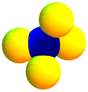
Figure 1: The sphere of last scatter viewed in the universal cover. The dark sphere marks the primary copy and the four lighter spheres are intersecting clones.

Previous attempts to detect topology in a finite universe have used statistics that are only sensitive to $T^{3}$ topologies[14, 15]. In contrast, our method is generic to all topologies that are locally homogeneous and isotropic (this includes all small FRW models). Importantly, the mapping from the surface of last scatter to the night sky is a conformal map. Since conformal maps preserve angles, the identified circles at the surface of last scatter would appear as equally rescaled, identified circles on the night sky. The angular radius and angular separation of each identified circle pair will depend on the geometry and topology of the universe, as will the number of pairs. If we are able to detect these circles, then their position, number and size can be used to determine the geometry and topology of the universe.

A second generic feature of topology is that it makes space globally anisotropic. This can be understood quite simply in the case of a three-torus in which looking along one of the axes brings you back around in a closed loop, but looking off-axis makes you wind round and round the space like the red strip around a barber pole. Thus, in a non-trivial topology, there are preferred directions. What is more surprising is that all but $T^{3}$ also make space globally inhomogeneous. In most topologies, the identifications of faces are made with twists (much like how a Mobius strip is constructed from a length of ribbon). Thus typical isometries involve a corkscrew type motion. Since the topologies violate global isotropy, this mixing of translations and rotations causes a violation of global homogeneity.

Unlike other inhomogeneous cosmologies, such as Tolman-Bondi universes which are locally inhomogeneous, these global violations of homogeneity and isotropy are not excluded. After all, we already know that the universe is weakly inhomogeneous and anisotropic on large scales – there is observable structure. Similarly, in the topologically interesting cosmologies, homogeneity and isotropy are violated only by the correlations between the structure that we observe – such as the fluctuations in the CMBR.

In principle, the locations of the identified circles can also be used to determine the orientation and location of the observer within the topology. More precisely, the topology can equally well be described in terms of many different fundamental cells, which share the same group structure, but represent different choices of generators for the fundamental group. The shape of the fundamental cell which an observer infers will depend on the observer’s location within the universe.

2.1 Searching for Circles in the Sky

Since the basic signature of topology is identified circles on the night sky, we have developed a statistical tool to detect these circles in all-sky maps of the CMBR. We begin by selecting two points on the night sky, $\overrightarrow{x},$ and $\overrightarrow{y}.$ We then draw circles of angular radius $\alpha$ around each point and consider all possible relative phases, $\phi_{*},$ between the two circles. Defining $T_{1}(\phi)$ and $T_{2}(\phi+\phi_{*})$ to be the temperature fluctuations around the circles centred at $\overrightarrow{x}$ and $\overrightarrow{y}$ respectively, we define the circle comparison statistic

$$S(\phi_{*})={<2T_{1}(\pm\phi)T_{2}(\phi+\phi_{*})>\over<T_{1}(\phi)^{2}+T_{2}(\phi+\phi_{*})^{2}>}\,,$$ (2)

where $<>=\int_{0}^{2\pi}d\phi$. The statistic ranges in the interval $[-1,1]$. Circles that are perfectly matched have $S=1$, while an ensemble of uncorrelated circles will have a mean value of $S=0$. By searching for circles that are either anti-phased or phased, we are able to detect both orientable and non-orientable topologies. Matched circles in orientable topologies have clockwise-anticlockwise temperature correlations while non-orientable topologies have a mixture of clockwise-clockwise and clockwise-anticlockwise correlations.

In any practical application, the number of truly independent measurements around each circle will be finite. An experiment with angular resolution $\Delta\theta$ provides roughly $N\simeq 2\pi\sin\alpha/\Delta\theta$ data points around each circle of angular radius $\alpha$. Neglecting the galaxy cut, the COBE-DMR instrument yields $N\simeq 36\sin\alpha$ pixels around each circle. In comparison, MAP should yield $N\simeq 1800\sin\alpha$ measurements around each circle using its highest frequency channel.

For circles which are identified due to topology, and which have their relative phase properly adjusted, $T_{1}$ should equal $T_{2}$ at each point around the circles. However, noise causes there to be a non-zero probability that $S\neq 1$. It is a reasonable approximation to treat the noise in each data pixel as an independent gaussian random variable with variance $\sigma_{\eta}^{2}$:

$$P(\eta)={1\over\sigma_{\eta}\sqrt{2\pi}}e^{-\eta^{2}/2\sigma_{\eta}^{2}}.$$ (3)

Assuming $T_{1}(\phi)=T(\phi)+\eta_{1}(\phi)$ and $T_{2}(\phi)=T(\phi)+\eta_{2}(\phi)$, where $\eta_{i}(\phi)$ is the noise, it is possible to derive an expression for the probability distribution of $S$ for matched circle pairs. The result is[16]

$$P^{m}(S)dS={\Gamma(N)2^{-N+1}\over\Gamma(N/2)^{2}}{(1+2\xi^{2})^{N/2}\over(1+(1-S)\xi^{2})^{N}}(1-S^{2})^{N/2-1}dS\,.$$ (4)

Here $\Gamma(z)$ is the gamma function and $\xi=\sigma_{s}/\sigma_{\eta}$ is the signal-to-noise ratio for the detector. The temperature fluctuations in the CMBR are taken to have a gaussian temperature distribution with variance $\sigma_{s}$. If $N$ is large, the distribution is peaked at

$$S^{m}_{max}={\xi^{2}\over 1+\xi^{2}}+{\cal O}(N^{-1})\,.$$ (5)

It is considerably harder to predict the temperature distribution for typical unmatched circles since fluctuations in the CMBR are known to have spatial correlations. We can make a crude estimate by ignoring these correlations and taking the temperature at each point on the sky to be an independent gaussian random variable. The probability distribution for unmatched circles is then[16]

$$P^{u}(S)dS={\Gamma(N)2^{-N+1}\over\Gamma(N/2)\Gamma(N/2)}(1-S^{2})^{(N-2)/2}dS\,.$$ (6)

This distribution is centred at $S=0$ and has ${\rm FWHM}\simeq(8\ln 2/N)^{1/2}$. Spatial correlations will tend to move the centre of the distribution toward larger $S$ and increase its width. Using the distributions (4) and (6) as a rough guide, we see that our statistic works best if the instrument has high resolution ($N$ large) and high signal-to-noise ($\xi$ large).

Figure 2: Simulated histograms for the circle statistic in a $T^{3}$ topology as measured by COBE-DMR. The dashed line is the histogram for unmatched circle pairs and the solid line is histogram for the matched circle pairs. The insert shows a detail of the region where matched circles might be detected.

When multiplied by the number of matched and unmatched circles pairs, $P^{m}(S)$ and $P^{u}(S)$ can be used to produce histograms of the circle statistic. Given an all-sky map with $M$ data points, the number of circle pairs of a given angular radius scales as $M^{2}$. Moreover, these have to be compared at $N\sim M^{1/2}$ different phasings. There will be $\sim M^{1/2}$ sets of circles of a given angular radius to compare, leading to a total sample that scales as $M^{3}$. The storage problem this poses can be alleviated somewhat if we only store the maximum value of $S(\phi_{*})$ for each circle pair. The distribution for unmatched circle pairs then becomes:

$$P^{u}_{\rm max}(S_{\rm max})=NP^{u}(S<S_{\rm max})^{N-1}P^{u}(S_{\rm max})\,.$$ (7)

Remembering that (4) and (7) overestimate the performance of the statistic, we can test to see if the COBE-DMR 4-year data[17] can be used to probe the topology of the universe. Crudely speaking, the instrument has an angular resolution of $\Delta\theta=10^{o}$ and reached a signal to noise ratio of $\xi=2$ after collecting data for 4 years. The optimal candidate topology for COBE to detect is a flat thee-torus with topology scale roughly equal to $R_{sls}$. The simulated histograms for this example are shown in Fig. 2. Even under the idealised conditions we have described, it is clear that detection would at most be marginal. The prospects are far brighter for the next generation of satellite missions. For example, MAP will provide all-sky coverage with a signal-to-noise of $\xi\sim 15$ at $\Delta\theta=0.5^{o}$. Any matched circles in these maps will be thrown into stark relief by our circle statistic.

Since the distribution of the circle statistic will be non-gaussian, Monte-Carlo simulations will be necessary to properly test the significance of a null detection or the significance of a potential detection. We are currently simulating the performance of the circle statistic by producing synthetic CMBR skies in both simply and multiply connected inflationary cosmologies and analysing them using the resolution and noise profile of the MAP satellite. Our preliminary results are very encouraging. Our confidence has been bolstered by the realization that the expected number of matched circle pairs for a generic small topology is very large (see section 4), and by Weeks’ observation[18] that just a few matched circle pairs can be used to find the generators of a topology’s fundamental group. This allows the entire topology to be reconstructed and the size and position of all the other circle pairs to be predicted. If these predictions agree with the data, then there will be absolutely no doubt about the result.

3 Circles in a $T^{3}$ universe

It is particularly easy to illustrate some of our ideas in a flat universe with three-torus topology. Using methods similar to those described in Ref.[14], we have simulated the CMBR in a cubic $T^{3}$ with topology scale $L=R_{sls}$. Our simulations were run at a resolution of $\Delta\theta=1.4^{o}$ using a flat Harrison-Zeldovich power spectrum and variable signal-to-noise. In Fig. 3 we display front and back views of the sphere of last scatter. Also marked are one pair of matched circles with angular radii of $\alpha=59.8^{o}$. Matched pairs were found by evaluating the circle statistic $S$ for all $2\times 10^{10}$ distinct circle pairs with angular radii in the range $10^{o}\leq\alpha\leq 90^{o}$. The number of distinct circle comparisons is finite as the search increment is fixed by the angular resolution of $\Delta\theta=1.4^{o}$.

In Fig. 4 we display the variation in CMBR temperature around each circle. Since the match is so good, we also show the temperature difference $T_{1}(\phi)-T_{2}(\phi)$. There is no phase offset for this matched pair. The graphs in Fig. 4 are drawn without noise. The noise is added when we simulate the detector response. In theory the match should be exact. The discrepancy is caused by what we call “pixel noise”. Since the

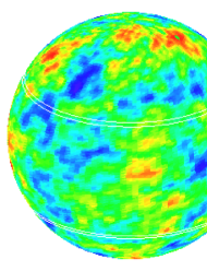
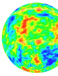
Figure 3: Views from opposite sides of the SLS globe. Two matched circles are marked.

Figure 4: (a) The CMBR temperatures around the two circles. The solid line is $T_{1}(\phi)$ and the dashed line is $T_{2}(\phi)$. (b) The temperature difference $T_{1}(\phi)-T_{2}(\phi)$.

angular resolution is finite, the circles we compare do not have exactly the right centrings or angular radii. Moreover, the temperature at each point around a circle is found by linear interpolation from the sky pixel temperatures. These effects combine to produce pixel noise. The pixel noise is reduced if we go to higher angular resolution. In addition, experimental data sets are usually oversampled, i.e. the data is recorded at an angular resolution substantially higher than the detector resolution. For COBE the data was collected at a resolution of $2.4^{o}$ while the true instrument resolution was $10^{o}$. Because of this oversampling, there is no information in the temperature gradient between adjacent pixels. Consequently, there will be no pixel noise coming from our temperature interpolation when we apply our search to real data sets.

The pair of matched circles have exactly the angular size and relative position we expect from the intersection of the sphere of last scatter with its nearest clone. In a flat universe the angular radius of a matched circle pair follows from simple trigonometry:

$$\alpha={\rm arccos}\left({X\over 2R_{sls}}\right)\,.$$ (8)

Here $X$ is the distance between us and the clone responsible for the matched circle. For a cubic $T^{3}$ with sidelength $L=R_{sls}$ there will be matched circle pairs with $\alpha=\{60^{o},45^{o},30^{0},0^{o}\}$ and multiplicities $\{3,6,4,3\}$.

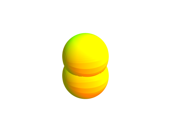
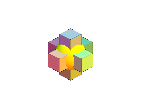
Figure 5: (a) The intersection that leads to the matched circle pair (b) The sphere of last scatter centred on the origin and the six nearest neighbours to the central fundamental cell.

The matched circles seen in Fig. 3 are due to the intersection shown in Fig. 5a. A partial tiling of the covering space by our six nearest neighbour fundamental cells is shown in Fig. 5b. The matched circles arising from these clones lie on faces of the fundamental cell. However, this is not true for all matched circle pairs. For example, the circles coming from the clones situated in the next-to-nearest neighbour cells (with $\alpha=45^{o}$) do not lie on faces of the fundamental cube.

We can evaluate the circle statistic $S(\phi_{*})$ for the matched pair under consideration. This is shown in Fig. 6 as a function of pixel offset $i=\phi_{*}/2\Delta\theta$. There is a clear peak at $\phi_{*}=0$ where the the statistic reaches the value $S(0)=0.975$. This should be compared to the FWHM of $S=0.21$ predicted by (6) for the distribution of unmatched circle pairs with the same radius. We are in the process of producing histograms for the complete search to confirm there is a clear detection. The results produced here were obtained by setting a threshold of $S_{cut}=0.95$ and only keeping circle pairs with $S>S_{cut}$. It was encouraging to find that no topologically unmatched pairs made the cut.

Figure 6: The circle comparison statistic, $S$, versus the pixel offset of the matched circle pair

Figure 7: The degradation in the circle match caused by detector noise.

We are also studying how other complications such as detector noise and the galaxy cut affect our ability to detect topology. In Fig. 7 we show how detector noise degrades the match. The graph suggest that a signal-to-noise of at least $\xi=5$ is required to get a good match. The next generation of CMBR satellite missions will far exceed this requirement.

4 Circles in a compact hyperbolic universe

The real power of the circle test is revealed when we apply it to models with compact hyperbolic spatial sections[10]. In these models it is very difficult to predict what the CMBR temperature fluctuations should look like as the inflationary perturbations are described by non-analytic functions[19]. This makes it difficult to place constraints on compact hyperbolic models using methods based on comparisons between predicted and observed CMBR maps[20, 21]. In contrast, the circle test requires no knowledge about what caused the temperature fluctuations on the sphere of last scatter. They could have been painted on by elves for all we care. The only difficulty we encounter is in trying to perform Monte-Carlo simulations of the circle search as these require synthetic sky maps.

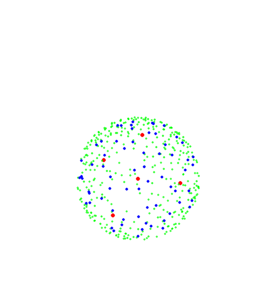
Figure 8: The distribution of our clones in the Thurston universe out to a radius of $3R_{curv}$. The large points are within one curvature radius, the medium sized points are within two curvature radii and the small points are within three curvature radii. The fundamental cell centred on the origin is also shown.

What we can do fairly easily is make some predictions about the number, size and distribution of circles in a generic small hyperbolic universes. The number, ${\cal N}$, of topologically matched circle pairs is given by the number of our clones within a proper distance of $D_{sls}$. A good estimate for this number is given by the ratio of the volume of space enclosed by a ball of radius $D_{sls}$ and the volume of the topology’s fundamental cell:

$${\cal N}={\pi(\sinh(2D_{sls}/R_{curv})-2D_{sls}/R_{curv})\over{\rm Vol}(\Sigma)}\,.$$ (9)

Once the radius of the ball exceeds the curvature radius, the volume of the ball, and hence the number of matched circles, grows exponentially with increasing radius. This makes the number of matched pairs a very sensitive function of the energy density. In Fig. 8 we show the distribution of clones in a model of the universe where the spatial sections are those of Thurston’s manifold[22]. The picture is drawn using Klein’s projective model of hyperbolic space, showing all clones out to a radius of $3R_{curv}$.

There are a two things to notice about this picture. The first is that most of our clones are at least $2R_{curv}$ away from the origin. The second is that the distribution is fairly isotropic (though this is not so evident in our 2-dimensional rendering of the 3-dimensional distribution). Using the fact that Thurston’s manifold has volume $0.981R_{curv}^{3}$, and recalling that $R_{sls}=R_{curv}{\rm arccosh}[(2-\Omega_{0})/\Omega_{0}]$, it is possible to estimate how the number of matched circles varies with the density parameter. This is shown in Fig. 9. Clearly, our chances of finding matched circles increases rapidly as the density of the universe decreases. In the observationally favoured range of $\Omega_{0}=0.3\rightarrow 0.4$, we expect to see tens of thousands of matched circles if we live in Thurston’s universe. Even if the fundamental cell has a volume as large as $1000R_{curv}^{3}$, we might still discover the topology of the universe.

Figure 9: The number of matched circles in Thurston’s universe as a function of the density parameter.

Using a little hyperbolic trigonometry we can predict the angular radius of the circles as a function of the proper distance $X$ between us and the clone responsible for the match:

$$\alpha={\rm arccos}\left({\cosh(X/R_{curv})-1\over\sinh(X/R_{curv})\tanh(R_{sls}/R_{curv})}\right).$$ (10)

In the limit $R_{curv}\rightarrow\infty$ we recover the flat space result (8). Since most of our clones will be situated near the boundary of the region $X<D_{sls}$, most matched circles will have small angular radii. In Fig. 10 we plot histograms showing the distribution of matched circle radii for Thurston’s universe with $\Omega_{0}=0.3$ and $\Omega_{0}=0.5$. The angular bins were taken to be one degree wide.

The circle statistic (2) works best when the number of pixels, $N$, around each circle is large. Since $N=360\sin\alpha/\Delta\theta$, the test works best for large circles. Our preliminary results indicate that we need $N\gtrsim 50$ to make a clear detection from a sky map with $\xi\sim 10$. Taking $\Delta\theta=0.5^{o}$, this tells us that only for $\alpha>4^{o}$ can we confidently identify individual circle pairs. The histograms in Fig. 10 suggest that this restriction would not seriously harm our ability to probe the topology of the universe. Moreover, because we expect many pairs of smaller circle pairs, and because, as pointed out by Weeks, any subset of two to three of them can be used to predict the location of all the others, we can use the self-consistency conditions to eliminate false positive identifications. We therefore expect to be able to probe somewhat, and perhaps substantially, below $\alpha=4^{o}$.

Figure 10: The distribution of matched circles as a function of angular size.

Compact hyperbolic models provide our best chance to discover the topology of the universe. Compared to a small flat universe of similar size, the exponentially larger volume of hyperbolic space leads to many more matched circles. While most of these circles have small angular radii, there should be enough large circles to make detection possible.

5 Prospects

The COBE 4-year map will not be our ultimate map of the microwave sky. NASA is currently making preparations to launch the MAP satellite in the year 2000[23]. MAP represents a ten-fold improvement in signal-to-noise and more than a thirty-fold improvement in resolution over the COBE-DMR map. ESA is also planing the PLANCK mission, to be launched in 2006[24]. PLANCK will have even higher resolution than MAP.

The topological signatures that we plan to search for should be easily detectable (if they are present) in the higher resolution, lower noise maps that will soon be available. If we find generic signals of topology, we will be able to identify the particular topology in which we live[18], where we are within the topology and which way is up. Using our synthetic sky maps, we will develop the technology to identify individual topologies in current and future data samples.

In summary, the possibility of non-trivial topology greatly widens and enriches the zoo of possible cosmologies. We have suggested that for generic small universes the ideal signal to look for is topologically identified circle pairs in the microwave background. We have devised a statistic to test for matched circle pairs and a strategy for performing the search. We are currently road-testing our search programs on simulated CMBR maps and hope to report our findings in the near future[16].

If we do detect the signature of finite topology, its implications would be profound and have great popular interest: we would learn that it’s small universe after all.

References

References

- [1] W. P. Thurston and J. R. Weeks, Scientific American, July ’84, 108; W. P. Thurston, The Geometry and Topology of 3-Manifolds (Princeton University Press, Princeton, 1978).
- [2] A. Einstein The Meaning of Relativity (Princeton University Press, Princeton, 1955), p. 108; J.A. Wheeler, Einstein’s Vision (Springer, Berlin, 1968).
- [3] G.F. Ellis, Q.J.R.Astron. Soc. 16, 245 (1975).
- [4] D. Atkatz and H. Pagels, Phys. Rev. D25, 2065 (1982); Ya. B. Zel’dovich and A. A. Starobinskii, Sov. Astron. Lett. 10, 135 (1984); Y.P. Goncharov and A.A. Bytsenko, Astrophys. 27, 422 (1989).
- [5] G. W. Gibbons, in this volume, Class. Quant. Grav. (1998); N. J. Cornish, G. W. Gibbons and J. R. Weeks, Cambridge Preprint DAMTP-R98/04, (1998).
- [6] D. Gabai, G. R. Meyerhoff & N. Thurston, MSRI Preprint # 1996-058, (1996).
- [7] L. A. Best, Can. J. Math. 33, 451 (1971).
- [8] J. R. Weeks, Ph.D. thesis, Princeton University (1985).
- [9] J. R. Weeks, SnapPea: A computer program for creating and studying hyperbolic 3-manifolds, available at http://www.geom.umn.edu:80/software.
- [10] N. J. Cornish, D. N. Spergel and G. D. Starkman, Phys. Rev. Lett. 77, 215 (1996).
- [11] D. N. Spergel, in this volume, Class. Quant. Grav. (1998).
- [12] M. Sasaki, T.Tanaka, K. Yamamoto, J. Yokoyama, Prog. Theor. Phys., 90, 1019 (1993); K. Yamamoto, M. Sasaki & T. Tanaka, ApJ, 455, 412 (1995); B. Ratra and P. J. E. Peebles, Phys. Rev. D52, 1837 (1995), M. Bucher, A.S. Goldhaber and N. Turok, Phys.Rev. D52, 3314 (1995); A. Linde, Phys.Lett.B351:99-104,1995.
- [13] M. Kamionkowski & D. Spergel, ApJ. 432, 7 (1994).
- [14] D. Stevens, D. Scott and J. Silk, Phys. Rev. Lett. 71, 20 (1993).
- [15] A. de Oliveira-Costa, G. Smoot and A. Starobinskii, Ap. J. 468, 457 (1996).
- [16] N. J. Cornish, D. N. Spergel and G. D. Starkman, in preparation.
- [17] C. L. Bennett et al., Astrophys. J. 464, L1, (1996).
- [18] J. R. Weeks, in this volume, Class. Quant. Grav. (1998).
- [19] N. J. Cornish, D. N. Spergel and G. D. Starkman, astro-ph/9708225 (1997).
- [20] J. R. Bond, D. Pogosyan and T. Souradeep, in this volume, Class. Quant. Grav. (1998).
- [21] J. J. Levin, in this volume, Class. Quant. Grav. (1998).
- [22] W. P. Thurston, Bull. Am. Math. Soc. 6, 357 (1982).
- [23] MAP homepage: http://map.gsfc.nasa.gov/html/.
- [24] Planck homepage: http://astro.estec.esa.nl/Planck/.