The Possibility of Thermal Instability in Early-Type Stars Due to Alfvén Waves

Abstract

It was shown by dos Santos et al. the importance of Alfvén waves to explain the winds of Wolf-Rayet stars. We investigate here the possible importance of Alfvén waves in the creation of inhomogeneities in the winds of early-type stars. The observed infrared emission (at the base of the wind) of early-type stars is often larger than expected. The clumping explains this characteristic in the wind, increasing the mean density and hence the emission measure, making possible to understand the observed infrared, as well as the observed enhancement in the blue wing of the $H_{\alpha}$ line. In this study, we investigate the formation of these clumps a via thermal instability. The heat-loss function used, $H(T,n)$, includes physical processes such as: emission of (continuous and line) recombination radiation; resonance line emission excited by electron collisions; thermal bremsstrahlung; Compton heating and cooling; and damping of Alfvén waves. As a result of this heat-loss function we show the existence of two stable equilibrium regions. The stable equilibrium region at high temperature is the diffuse medium and at low temperature the clumps. Using this reasonable heat-loss function, we show that the two stable equilibrium regions can coexist over a narrow range of pressures describing the diffuse medium and the clumps.

1 Introduction

As demonstrated first by Lucy & Solomon (1970), the radiative momentum absorbed by UV spectral lines is able to initiate stellar winds, since the radiative line acceleration exceeds the gradient by a large factor. The first model to derive mass–loss rates ($\dot{M}$) and flow speeds in good agreement with observations was that of Castor, Abbott & Klein (1975) (CAK). One of the major difficulties presented by the radiation driven wind theory is the momentum problem in WR stars, which can be described using the ratio $\eta=({\dot{M}}v_{\infty})/(L_{*}/c)$, where $v_{\infty}$ is the terminal velocity and $L_{*}$ the star luminosity. Barlow et al. (1981) found that in WR stars $\eta$ ranges from 3 to 30. This means that there is about an order of magnitude more momentum in the wind than in the radiation field. It was assumed that every stellar photon transfers its momentum, $h\nu/c$, only once (single scattering), but even with multiple scattering of the photons one obtains ${\dot{M}}v_{\infty}>5L_{*}/c$. To get around the momentum problem, one cannot simply appeal to a larger luminosity, because the values that are used cannot be near the Eddington limit (Cassinelli & van der Hucht 1987).

Following the suggestion that there may be appreciable magnetic fields in WR stars larger than 1000 G (Mahesvaran & Cassinelli 1988; Poe et al. 1989), it was suggested that the wind in a WRN5 star, for instance, can be driven by Alfvén waves (see Hartmann & Cassinelli 1981). They assumed B=20,000 G and a mechanical flux of Alfvén waves of $\Phi_{w}=1.1\times 10^{14}\;{\rm erg/cm}^{2}{\rm s}$ (this work did not take into account the contribution of the radiation pressure on the lines).

As implied by the work of Willis (1991), an additional mechanism to radiation pressure may be required to initiate the high WR mass–loss, although thereafter the winds may be radiatively accelerated. In this context, dos Santos et al. (1993a,b) proposed a model for mass–loss in WR stars, where both a flux of Alfvén waves and radiation pressure are considered. The model is a fusion of the Alfvén wave wind model of Jatenco–Pereira & Opher (1989a,b) and the radiation pressure CAK model. In the model an effective escape velocity is used, which takes into account the CAK power index expressing the effect of all lines, possible nonsolar abundances, and the finite size of the star disk. Their work indicates that Alfvén waves, acting jointly with radiation pressure, provide the necessary energy and momentum for the wind, with reasonable Alfvén fluxes and magnetic fields.

Early-type stars show superionization lines O VI, N V, $H_{\alpha}$ and X-rays, that cannot be explained by the high temperature star. Applying the coronal zone model to the winds of early-type stars, Cassinelli & Olson (1979) derived the ionization conditions expected in the wind of $\zeta$ Pup. The results of this study explain very well the persistence to low effective temperatures of the strong lines of O VI, N V, C IV and Si IV.

Since Abbott et al. (1984), one knows that the observed IR emission is often larger than expected from a homogeneous wind. From that time it was pointed out that the clumping in the wind, increases the mean density and hence the emission measure. Clumping can also explain an observed enhancement in the blue wing of the $H_{\alpha}$ line. The narrow absorption components are likely to be direct manifestations of dense clumps. Now, the existence of these clumps is largely known in many individual hot stars, and clumping may be important in all hot stars with winds (Hillier 1991; Robert 1994; Moffat & Robert 1994; Massa et al. 1995; Brown et al. 1995; Moffat 1994,1996; Eversberg et al. 1996).

In principle, it can be said that the series of papers by Owocki, Rybicki and Castor (Owocki & Rybicki 1984, 1985, 1986, 1991; Owocki et al. 1988; Rybicki & Owocki 1990), which contains numerical hydrodynamic calculations, show that the radiation driven winds are violently unstable and that the consequent shocks can explain the X-ray emission of early-type stars, moreover the clumping explains the infrared emission excess and the formation of narrow absorption components. These models qualitatively explain the hot stars wind structure, and the role of Alfvén wave damping in these winds is an open question, as noted by these authors. In this sense, our model is an attempt to explain the inhomogeneities of hot star winds using thermal instability in the presence of Alfvenic heating.

The propagation and transmission of magnetohydrodynamic waves through stellar atmospheres and winds has attracted considerable interest, because of its relevance to the questions of chromospheric and coronal heating and wind acceleration (Leer et al. 1982). In order to accelerate a wind efficiently, the waves must be able to propagate without much reflection or attenuation up to the sonic point, because any addition of momentum below that point essentially goes to increase the mass flux but not the asymptotic wind speed (Leer et al. 1982). On the other hand, as commented by Velli (1993), waves reflected and/or having a nonlinear evolution in the lower atmospheric layers, contribute to the nonradiative heating through turbulent decay.

We study here a mechanism to form condensations in the base of early-type star winds. The basis for this approach is the work of dos Santos et al. (1993a,b) – a wind acceleration model for Wolf-Rayet stars where Alfvén waves act jointly with the radiation pressure. Considering the above scenario, with special attention to the clumping features, our intent is to study the relevance of a flux of Alfvén waves in the hot medium present in the base of WR winds, in order to understand the formation of the clumping features. As the magnetic field is more effective in the base of the wind (see dos Santos et al. 1993a), we have there a wave flux, resulting in a model that could explain clumps in this region. We consider a thin hot corona atmosphere, which corresponds to the X-rays observed, with a temperature of $\sim 10^{7}{\rm K}$, and density of $\sim 2\times 10^{13}{\rm cm}^{-3}$ (see van der Hucht 1992). In principle, the thermal instability process presents, as a result, the clumps observed, and we call these clumps the cool atmosphere ($\sim 10^{4}{\rm K}$ and $\sim 10^{3}$ times denser than the hot medium) (for instance, Brown et al. 1995). Our final goal is to demonstrate the stability of the base of the wind that has “cool” ($\sim 10^{4}{\rm K}$) clouds and “hot” ($\sim 10^{7}{\rm K}$) intercloud medium coexisting at the same pressure.

2 Physical Mechanisms

In general, astronomical objects are formed by self-gravitation. However, some objects cannot be explained by this process. For these objects the gravitational energy is smaller than the internal energy. In these cases, it is assumed that the internal pressure is balanced by the pressure of the external medium. These objects (that cannot be explained by self-gravitation) are formed from the medium by some kind of condensation process not involving gravitation. Parker (1953) argued that, if the thermal equilibrium of the medium is a balance between energy gains and radiative losses, instability results if, near equilibrium, the losses increase with decreasing temperature. Then, a cooler-than-average region cools more effectively than its surroundings, and its temperature rapidly drops below the initial equilibrium value.

Following Lucy & Solomon (1970), for a given ionization potential, $\chi_{r}=h\nu_{r}$, the photoionization rate, $\Gamma_{r}$ is a function only of the radiation temperature, $T_{r}$; the collisional rate, $\Gamma_{c}$, on the other hand, is determined by the electron density, $n_{e}$, and the electron temperature, $T_{e}$. The ratio of the two rates is

$$\frac{\Gamma_{r}}{\Gamma_{c}}=\frac{\left[\int_{\nu_{r}}^{\infty}\frac{4\pi B_{\nu}(T_{r})}{h\nu}a_{\nu}d{\nu}\right]}{n_{e}\langle\sigma_{r}v_{e}\rangle}\;\;\;,$$

here $\sigma_{r}$ is the cross–section for collisional ionizations, $v_{e}$ the electron velocity, and $a_{\nu}$ the photoionization cross–section. B$\ddot{{\rm o}}$hm (1960) has given approximations for these quantities from which one derives

$$\frac{\Gamma_{r}}{\Gamma_{c}}\simeq 6\times 10^{10}\frac{T_{e}^{1/2}\chi_{r}^{3}}{n_{e}}\;\;\;,$$

where $T_{r}=T_{e}$, $h\nu_{r}/kT_{r}\geq 1$, approximately, and the units of $\chi$ are electron volts.

Applying these results to the ionization of C III ions, for instance, $\chi_{r}=47.9$ eV with $\log T_{eff}=4.5$. Taking $T_{e}$ (in the hot atmosphere) $\approx 10^{3}T_{eff}$, and $n_{e}=2\times 10^{13}{\rm cm}^{-3}$, one obtains ${\frac{\Gamma_{r}}{\Gamma_{c}}}=3\times 10^{5}$ (for lower density the ratio is even higher), so that collisional ionization may be completely neglected.

Considering a thermal instability in an isobaric regime (e.g., Field 1965) (internal pressure balanced by the external pressure), we looked for a set of physical parameters that, at equilibrium $[H(T,n)=0]$, show three equilibrium regions: one stable region representing the diffuse medium; one unstable region; and another stable region representing the condensations. The energy gains considered are: heating by photoionization-recombination, $H_{r}$; Compton heating, $H_{c}$; and Alfvén wave heating, $H_{A}$. These gains are balanced by the following radiative loss processes: cooling via thermal bremsstrahlung, $H_{b}$; inverse Compton cooling (this term is computed jointly with $H_{c}$); and collisional excitation followed by resonance line emission, $H_{rl}$.

2.1 Bremsstrahlung Losses

The total amount of energy radiated in free-free transitions, per ${\rm cm}^{3}$ per ${\rm sec}$, in the case of a Maxwellian distribution of velocities, is

$$H_{b}=-\left(\frac{2\pi kT}{3m_{e}}\right)^{1/2}\frac{2^{5}\pi e^{6}}{3hm_{e}c^{3}}Z^{2}n_{e}n_{i}{\bar{g}}_{ff}$$

$$H_{b}=-1.42\times 10^{-27}Z^{2}n_{i}n_{e}T^{1/2}{\bar{g}}_{ff}$$

$$H_{b}=-\lambda_{b}T^{1/2}n^{2}\;.$$ (1)

The quantity ${\bar{g}}_{ff}$ appearing above is a correction factor required for precise results. Its value is generally about unity (Spitzer 1978), and $\lambda_{b}=2.4\times 10^{-27}$. Hereafter $n_{e}\equiv n$, the number density.

2.2 Resonance Line Emission

Raymond et al. (1976) calculated a radiative cooling coefficient for a low density gas, optically thin, with cosmic abundances, between the temperatures of $10^{4}{\rm K}$ and $10^{8}{\rm K}$, which we adopt in this work. A good fit to radiative losses, in this temperature range, due to electron excitation of resonance transitions in common metal ions (${\rm erg/cm}^{3}{\rm s}$) is (Raymond et al. 1976; Mathews & Doane 1990),

$$H_{rl}\;=\;-\;\frac{a\;T^{p}}{1\;+\;b\;T^{q}}\;n^{2}\;\;,$$ (2)

with $a=1.53\times 10^{-27}$, $b=1.25\times 10^{-9}$, $p=1.2$, and $q=1.85$.

2.3 Photoionization-Recombination Heating

An approximate equation to express the residual heating due to radiative ionization followed by recombination, in ${\rm erg/cm}^{3}{\rm s}$, is

$$H_{r}\;=\;\alpha_{B}\;(T){\rm max}\;\left[0,\langle h\nu\rangle_{i}-h\nu_{o}-f3k_{B}T/2\right]\;n^{2}\;,$$ (3)

where $\langle h\nu\rangle_{i}$, the mean energy of ionizing photons, is

$$\langle h\nu\rangle_{i}=\frac{\sum n_{j}h\nu_{j}}{\sum n_{j}}=\frac{n_{H}kT_{H}+n_{L}kT_{L}}{n_{H}+n_{L}}\;,$$

$n_{L}$ and $n_{H}$ are the numerical densities of photons of the low and high temperature regions, respectively, given by

$$n_{L}=\frac{\sigma T_{L}^{4}}{k_{B}T_{L}c}\;{\rm with}\;T_{L}=T_{*}\;,$$

and

$$n_{H}=\frac{[H_{rl}(T_{H},n_{H})+H_{b}(T_{H},n_{H})]tR_{*}}{kT_{H}c}\;,$$

where $\alpha_{B}=2.60\times 10^{-13}$ $(T/10^{4})^{-0.8}$ $cm^{3}$ $s^{-1}$ is the recombination coefficient, and $h\nu_{o}$ the ionization potential of hydrogen. In the above equations $n_{H}$ and $T_{H}$ are the density and temperature of a high temperature region, $n_{L}$ and $T_{L}$ are the same for a low temperature region, and $tR_{*}$ is the region thickness. Each recombination results in a loss of energy $f3k_{B}T/2$ from the thermal energy of the plasma, with $f\approx 0.43$ (Mathews & Doane 1990).

The recombination expression, eq.(3), is an approximated one. Equation (3) states that we have recombination only when the average energy of the photons, $\langle h\nu\rangle_{i}$, is sufficiently high such that ionization can occur, that is, when $\langle h\nu\rangle_{i}$ is greater than $h\nu_{0}\;+\;f3k_{B}T/2$ (i.e., the sum of the ionization potential plus the average energy of the electron that is liberated).

2.4 Compton Heating-Cooling

We have to estimate the number and frequency of the photons acting in the immediate neighborhood of the star surface and anywhere in the star atmosphere. Taking into account the interaction between thermal electrons and the radiation field, photons with lower frequency, come from a cooler optically thick region, the stellar continuum. Their flux is $\sigma{T_{*}}^{4}$, and then, for these photons, we have

$$\frac{L_{bL}}{4\pi R{{}_{L}}^{2}}=\sigma{T_{*}}^{4}\;\;\;.$$

On the other hand, a hot region of thickness $tR_{*}$ (optically thin), at temperature $T_{H}$ causes heating in the medium via, principally, thermal bremsstrahlung and resonance line emission [$H_{b}(T,n)$ and $H_{rl}(T,n)$]. Hence, for these photons,

$$\frac{L_{bH}}{4\pi R_{H}^{2}}=\left[H_{b}(T_{H},n_{H})+H_{rl}(T_{H},n_{H})\right]tR_{*}\;\;\;.$$

The complete expression for Compton heating and cooling is then

$$H_{c}\;=\;\frac{4\;k_{B}\;\sigma_{T}}{m\;c}\frac{n}{c}\left\{\left[(T_{H}-T)\frac{L_{bH}}{4\pi R_{H}^{2}}\right]+\left[(T_{L}-T)\frac{L_{bL}}{4\pi{R_{L}}^{2}}\right]\right\}\;\;,$$ (4)

which is similar to the expression usually adopted, for instance by Mathews & Doane (1990). In the above equations $k_{B}$ is the Boltzmann constant, $\sigma_{T}$ the Thompson cross section, $\sigma$ the Stefan-Boltzmann constant, $n$ the number density, $m$ the electron mass, $T$ the temperature, $L_{b}$ the bolometric luminosity, $c$ the light speed, $T_{*}$ the stellar temperature and $R_{*}$ the stellar radius.

3 Damping and heating from Alfvén waves

Alfvén waves in a early-type star, whose winds are primarily radiatively driven, are subject to damping (or amplification) as described, for example, by MacGregor (1996). In this case, the dispersion relation for Alfvén waves in a radiatively driven wind, is $k^{2}v_{A}^{2}=\omega^{2}-i\omega\omega_{0}$ (instead of $k^{2}v_{A}^{2}=\omega^{2}$), where

$$\omega_{0}=\frac{2\pi\kappa_{L}\nu_{L}}{3c^{2}}\frac{dI_{*}(\nu)}{d\nu}\qquad,$$

$I_{*}(\nu)$ is the intensity of the photospheric radiation field, $\nu_{L}$ is a line rest frequency and $\kappa_{L}$ is the line mass absorption coefficient. If $dI_{*}(\nu)/d\nu>0$ then the Alfvén wave is amplified, while if $dI_{*}(\nu)/d\nu<0$ the Alfvén wave is damped. Although, as MacGregor (1996) noted, “the presence of such radiatively modified Alfvén waves in the flow has yet to be explored”. We apply in the present investigation, the dampings described below with their heatings.

The damping mechanisms that we assume here were used before in many astrophysical objects: protostellar, late-type stars and solar winds   (Jatenco-Pereira & Opher 1989a,b); galactic and extragalactic jets (Opher & Pereira 1986; Gonçalves et al. 1993b); early-type stars (dos Santos et al. 1993a,b); broad line regions of quasars (Gonçalves et al. 1993a, 1996); cooling flows of galaxy clusters (Friaça et al. 1997) and others.

3.1 Nonlinear damping

Parallel Alfvén waves are purely transverse and there is no important linear damping. The damping that does occur is not linear and it arises from a beat wave (two circularly polarized parallel propagating waves) which contains a longitudinal field component and a longitudinal gradient in the magnetic field. This results in a nonlinear damping of both electrostatic and magnetostatic components i.e. transient time damping.

V$\ddot{{\rm o}}$lk & Cesarsky (1982) derived an equation that represents the unsaturated Landau damping, in the case of nonlinear two-wave interaction, that can be written as

$$\;\;\Gamma(k)=\frac{1}{4}\sqrt{\frac{\pi}{2}}\xi\bar{k}v_{s}\Im\;,$$

where $\Im$ is the energy density in waves normalized to the ambient magnetic energy density, $B_{0}^{2}/8\pi$ (Lagage & Cesarsky 1983). Using $\Im={\frac{\rho\langle\delta v^{2}\rangle}{B_{0}^{2}/8\pi}}$ and $\bar{k}={\frac{\varpi}{v_{A}}}$, we obtain:

$$\Gamma_{nl}={\frac{1}{4}}{\ \sqrt{\frac{\pi}{2}}}\xi\bar{w}\left(\frac{v_{s}}{v_{A}}\right)\frac{\rho\langle\delta v^{2}\rangle}{B_{0}^{2}/8\pi}\;\;\;,$$ (5)

where $\xi=5-10$ and $v_{s}$ is the sound velocity.

3.2 Turbulent damping

There are strong evidences favoring anisotropic, supersonic and compressible turbulence in WR winds. Since all WR stars observed intensively so far do behave similarly, and WR stars are extreme manifestations of winds in hot luminous stars, it is possible or even likely that all hot-star winds show the same basic phenomenon (Moffat et al. 1994 and references therein). A necessary (but not sufficient) condition that one is dealing with turbulence is that the Reynolds number be $Re>>1$. For an expanding wind, with $v_{w}(r)$ the expansion speed and $r$ the distance from the star, one has:

$$Re\approx\frac{rv_{w}(r)}{\nu_{thermal}}\approx\frac{r}{l_{mfp}}\frac{v_{w}(r)}{v_{s}}\;\;\;,$$

where $\nu$ is the viscosity, $l_{mfp}$ the mean free path of the average particle in the medium. Thus, with typical WR wind values, where the observed lines form, $Re$ is much higher than $1$, so turbulence is likely to exist if there is a driving force.

Hollweg (1986) considered a new hypothesis for the nonlinear wave dissipation of Alfvén waves. The hypothesis is that the wave dissipates via turbulent cascade, or, this hypothesis concerns the consequences of the Alfvén wave dissipation in terms of wave-particle interactions, where the required power at high frequencies is presumably supplied via turbulent cascade. Then, exploiting the similarity of $P_{{\rm B}}\propto k^{-5/3}$ and Kolmogorov turbulence in ordinary fluids, the plasma volumetric heating rate associated with the cascade is given by:

$$E_{H}=\frac{\rho\langle\delta v^{2}\rangle^{3/2}}{L_{{\rm corr}}}\frac{}{},$$ (6)

where $\rho$ is the mass density, $\langle\delta v^{2}\rangle$ is the velocity variance associated with the wave field, and $L_{{\rm corr}}$ is a measure of the transverse correlation length. A subhypothesis is that the correlation length scales as the distance between magnetic field lines,

$$L_{{\rm corr}}\propto B^{-1/2}\frac{}{}.$$

In spite of $L_{{\rm corr}}$ being a free parameter, the model comes close to the notion of a Kolmogorov-like cascade to small scales. The waves themselves are here regarded as the source of the heating. In this case $\langle\delta v^{2}\rangle$ only includes the power associated with Alfvenic fluctuations. Similarly, $L_{corr}$ concerns the correlation length of the Alfvenic fluctuations. Finally, in terms of damping length, we have

$$L_{t}=L_{{\rm corr}}\;v_{A}{\langle\delta v^{2}\rangle}^{-1/2}\frac{}{},$$ (7)

(Hollweg 1986, 1987).

3.3 Alfvén wave heating

Data of the last 10 years show us that early–type stars can be separated in two groups: magnetic stars, with surface strengths of a dipole or quadrupole magnetic field of $B\approx n(10^{2}-10^{3}){\rm G}$, $n=2,3,...7$; and normal stars, with $B\approx 1-100\;{\rm G}$. The magnetic field strength increases towards the center of the star and in the core is $\approx(0.1-10)\times 10^{6}{\rm G}$, depending on the stellar mass (Dudorov 1994; Bohlender 1994). The origin of these fields is an open question, and two theories compete to explain it: dynamo and fossil theories (Moss 1994).

Consider now a collapsing cloud. For the collapsing cloud the cross sectional area perpendicular to a magnetic field, $A$, is $\propto\rho^{-{\frac{2}{3}}}$ and $B$ $\propto A^{-1}\propto\rho^{{\frac{2}{3}}}$, where $\rho$ is the mass density of the gas and $B$ is the magnetic field. The damping length in each case is $L=v_{A}/\Gamma$ (i.e., the ratio between the Alfvén velocity and the damping rate). Knowing that $v_{A}=B/\sqrt{4\pi\rho},\;\;\rho\langle\delta v^{2}\rangle\;\propto\;\Phi_{w}/v_{A}$, where $\Phi_{w}$ is the wave flux and $\Phi_{w}\;\propto\;\rho^{2/3}$, we write the nonlinear Alfvenic heating as:

$$H_{nl}\;=\;\Phi_{w}/L_{nl}\;=\;\frac{\Phi_{w}}{v_{A}}\Gamma_{nl}\;\propto\;\frac{\Phi_{w}}{v_{A}^{2}}\frac{\rho\langle\delta v^{2}\rangle}{B^{2}}\;\propto\;\rho^{-1/2}\;\;\;;$$ (8)

and for the turbulent Alfvenic heating,

$$H_{t}=\Phi_{w}/L_{t}\;\propto\;\Phi_{w}B^{1/2}\frac{{\langle\delta v^{2}\rangle}^{1/2}}{v_{A}}\;\propto\;\rho^{7/12}\;\;\;;$$ (9)

following equations (5) and (7).

The sum of the contributions from Compton and inverse Compton, photoionization-recombination, bremsstrahlung and resonance line emission, is about $10^{-22}n^{2}$. We are adopting $n_{H}$ (the density of the hot atmosphere)$=2\times 10^{13}{\rm cm}^{-3}$, resulting $10^{-22}n^{2}\approx 4\times 10^{4}{\rm erg/cm}^{3}{\rm s}$. We then normalize the Alfvenic heatings using $F_{nl},F_{t}=10^{2}-10^{5}{\rm erg/cm}^{3}{\rm s}$. So,

$$H_{nl}=F_{nl}\left(\frac{n}{2.0\times 10^{13}}\right)^{-{\frac{1}{2}}}$$ (10)

and

$$H_{t}=F_{t}\left(\frac{n}{2.0\times 10^{13}}\right)^{\frac{7}{12}}\;\;\;.$$ (11)

3.4 The overall heating/cooling behavior

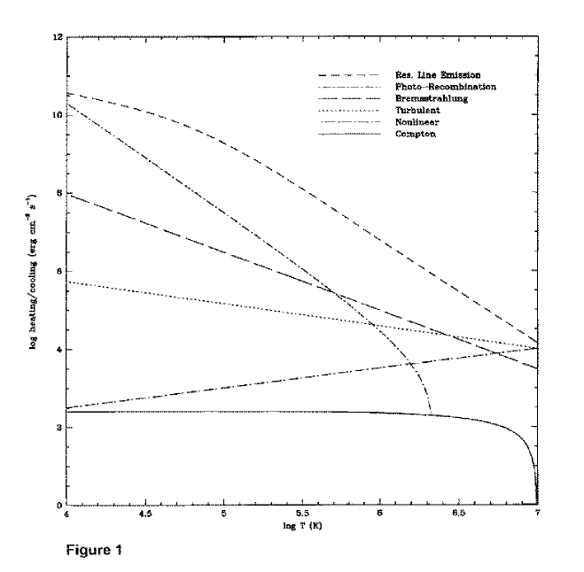
Figure 1: The module of the heating/cooling processes, for $\log P_{H}=4.74$ ($P_{H}=5.5\times 10^{4}{\rm dyn/cm}^{2}$), $F_{nl}=F_{t}=F_{A}=10^{4}$ and $t=0.2$ (as in Fig. 2 - 5, where the thermal instability process occurs for $T_{L}<T<T_{H}$ with $T_{L}=3\times 10^{4}\;K$ and $T_{H}=10^{7}\;K$).

In order to make clear the relevance of each heating/cooling process in the overall balance we plot, in Figure 1, the module of the heating or cooling due to: resonance line emission; photoionization-recombination; thermal bremsstrahlung; Alfvenic turbulent and nonlinear heatings; and Compton interactions, as a function of temperature, in units of ${\rm erg/cm}^{3}{\rm\;s}$.

The first characteristic we note from Figure 1 is the fact that resonance line emission is the most important cooling. In fact it dominates over all the other processes in this range of temperature. Another aspect is that we are using only the contribution of the photoionization-recombination processes that produces heating. This mechanism is not considered at temperatures higher than $\log T\simeq 6.3$. At these high temperatures it appears as cooling (see also eq. (3)).

From the physics of Alfvén wave heating, it is clearly not temperature dependent (eqs. (10) and (11)), beyond a dependence on the density which implicitly scales inversely to temperature, keeping P fixed. Then, as Alfvén heating is proportional to $n^{\alpha}$ ($\alpha=-1/2,7/12$), at a given pressure, we have this heating proportional to $T^{-\alpha}$, as can be seen from Figure 1.

4 Results

The complete heating–cooling function, $H(T,n)$, including the physical processes discussed above, is:

$$H(T,n)=-\lambda_{b}T^{{\frac{1}{2}}}n^{2}-\frac{aT^{p}}{1+bT^{q}}n^{2}+\frac{4k_{B}\sigma_{T}n}{mc^{2}}\times$$

$$\left\{(T_{H}-T)\left[\frac{}{}H_{b}(T_{H},n_{H})+H_{rl}(T_{H},n_{H})\right]tR_{*}+(T_{L}-T)\frac{}{}\sigma T_{*}^{4}\right\}+$$

$$\alpha_{B}(T){\rm max}\left[0,\langle h\nu\rangle_{i}-h\nu_{o}-\frac{f3k_{B}T}{2}\right]n^{2}\ +\ H_{A}\ \ \ ,$$ (12)

with $H_{A}$ assuming the form of $H_{nl}$ and $H_{t}$, given by equations (10) and (11). All the constants in (12) are in $cgs$ units.

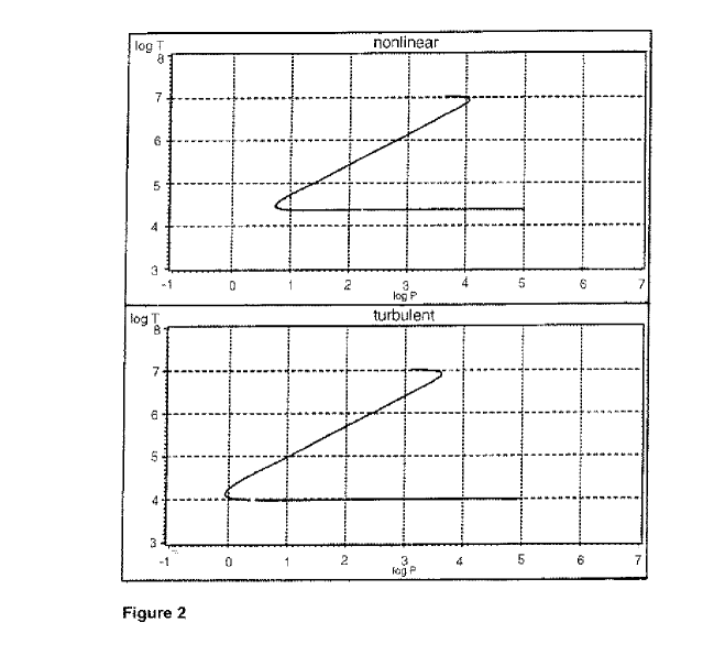
Figure 2: The $\log T\times\log P$ diagram ($H(T,n)\approx 0$), with $F_{A}=10^{2}$: nonlinear and turbulent Alfvenic heatings.

Figures 2 to 5 show the balance between energetic gains and radiative losses (from equation (12)), i.e., the equilibrium of $H(T,n)(\approx 0)$ in a $\log P-\log T$ diagram. For this calculation we assume $n_{H}=2.0\times 10^{13}{\rm cm}^{-3}$, $T_{H}=1.0\times 10^{7}{\rm K}$, $T_{L}=T_{*}=3.0\times 10^{4}{\rm K}$; $R_{*}=12R_{\odot}$ and $t=0.2$.

As we are forming clouds, via thermal instability, from the hot atmosphere ($n_{H}=2.0\times 10^{13}{\rm cm}^{-3}$ and $T_{H}=1.0\times 10^{7}{\rm K}$), we performed calculations in order to find, for each temperature, the density that corresponds to the balance ($H(n,T)\approx 0$). From the isobaric instability criterion, we need the clouds and the hot medium coexisting at the same pressure. In the hot atmosphere the pressure is $P_{H}=2n_{H}kT_{H}\approx 5.5\times 10^{4}{\rm dyn/cm}^{2}{\rm s}$. We then want to verify the possibility of forming clouds ($\approx 10^{4}{\rm K}$, cool and dense atmosphere) at pressures near the characteristic pressure of the hot medium.

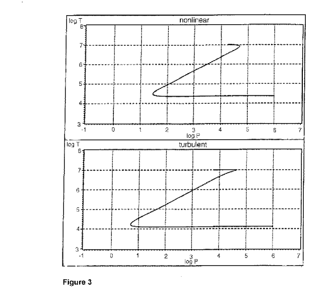
Figure 3: The $\log T\times\log P$ diagram ($H(T,n)\approx 0$), with $F_{A}=5\times 10^{3}$: nonlinear and turbulent Alfvenic heatings.

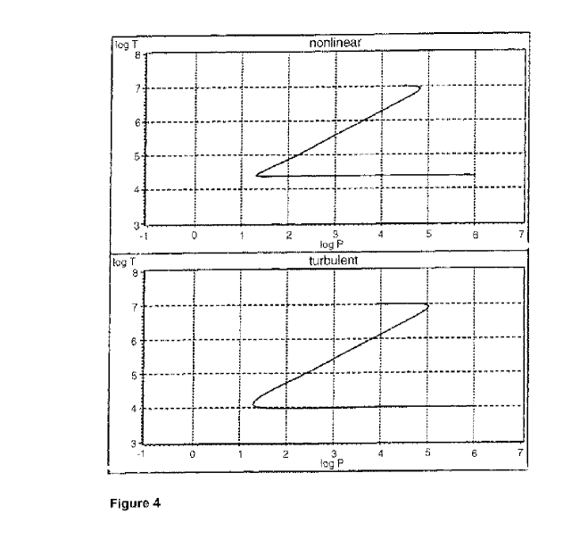
Figure 4: The $\log T\times\log P$ diagram ($H(T,n)\approx 0$), with $F_{A}=10^{4}$: nonlinear and turbulent Alfvenic heatings.

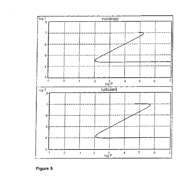
Figure 5: The $\log T\times\log P$ diagram ($H(T,n)\approx 0$), with $F_{A}=10^{5}$: nonlinear and turbulent Alfvenic heatings.

In Figures 2 – 5 we assume a single value of $F_{A}$ for the two Alfvenic heating terms, nonlinear ($F_{nl}$) and turbulent ($F_{t}$). In Figure 2, we have the equilibrium diagram in terms of pressure and temperature adopting $F_{A}=10^{2}$. This figure shows us the coexistence of the two-phase equilibrium at pressures lower than the characteristic pressure of the hot atmosphere (${\rm\log}P_{H}=4.74$). For this value of $F_{A}$, the nonlinear heating (in the case in which the Alfvenic heating contribution to the overall heating-cooling function is the nonlinear one), as well as the turbulent heating, are insufficient to permit the coexistence of the hot and cool atmospheres, at appropriate pressures. Analyzing Figure 3 ($F_{A}=5\times 10^{3}$), we observe that both cases (nonlinear and turbulent) are satisfactory, in order to permit cloud formation via thermal instability, since they reach the pressure desired. Finally, in Figure 4 ($F_{A}=10^{4}$) and Figure 5 ($F_{A}=10^{5}$), the cool and hot stable solution can be found at the pressure desired (the reference pressure and higher pressures) in the two cases. In addition, it is clear that turbulent Alfvenic heating does a better job than nonlinear heating, since the pressure range of the coexistence of both stable equilibria is bigger (see bottom panel in Figures 4 and 5) in the case of this Alfvenic heating.

5 Discussion and Conclusions

Our results can be discussed in terms of the efficacy of the Alfvenic heatings in forming condensations near the surface of WR stars due to thermal instability. This efficiency is included in the scaling factor $F_{A}$, that is equal $F_{nl}$ or $F_{t}$ in Figures 2 - 5.

We consider in this study a heuristic derivation of the expressions for Alfvenic heatings. The nonlinear and turbulent Alfvenic heatings represent extreme opposite dependencies of these heatings on density. Comparing this behavior we have: turbulent heating ($H_{t}\propto n^{7/12}$) which deposits more energy when the density is higher; on the other hand, nonlinear heating ($H_{nl}\propto n^{-1/2}$) deposits more energy when the density is lower. These behaviors also can be seen from Figure 1 in which cooler regions are denser than hotter ones (that figure was plotted for a fixed pressure ($P_{H}$), then, the nonlinear heating curve is a decreasing function of density, opposite to the case of turbulent heating). Due to the completely different behavior of these heatings, the results from each one are very different (see plots 2 to 5 with the equilibrium solution for our models). Despite the fact that the Alfvenic heatings do not work in the cool solution, as well as in the hot one, results with nonlinear heating produce the cool condensations at about $2.2\times 10^{4}{\rm K}$, while the results with turbulent heating show cooler low temperature solutions ($\sim 1.0\times 10^{4}{\rm K)}$. Noting also the way that each process scales with P, at fixed T, one can understand why the stable hot solution has a narrower range in pressure than the stable cool solution, in all figures of equilibrium (figures 2 - 5).

In the work of dos Santos et al. (1993a), the principal emphasis was to determine the terminal velocity of the Wolf-Rayet star winds, using a model which had radiation pressure and Alfvén waves driving the wind. The initial Alfvén wave flux, $\Phi_{w}$, required was $\approx 5.6\times 10^{12}{\rm erg/cm}^{2}{\rm s}$. Using this value for the wave flux, we can estimate the damping length for the Alfvén waves. As in the derivation of Alfvenic heatings (subsection 3.3), $\Phi_{w}$ is equal to $H_{A}L_{A}$. Adopting, for example, the maximum pressure in which the stable two-phase equilibrium exists, in Figure 5b, $P_{H}\simeq 5\times 10^{5}\;{\rm dyn/cm}^{2}$, the turbulent Alfvenic heating for the formed clouds is $\sim 1.9\times 10^{7}\;{\rm erg/cm}^{3}{\rm s}$. Then,

$$L_{t(min)}=\frac{\Phi_{w}}{H_{t}}\simeq{\frac{5.6\times 10^{12}}{1.9\times 10^{7}}}\simeq 3\times 10^{5}\;{\rm cm}.$$

Taking now the minimum value for the pressure in the cloud in Figure 5b, $P\simeq 3.9\times 10^{4}{\rm dyn/cm}^{2}$, the turbulent Alfvenic heating is $\sim 4\times 10^{6}{\rm erg/cm}^{3}{\rm s}$. We then have

$$L_{t(max)}=\frac{\Phi_{w}}{H_{t}}\simeq{\frac{5.6\times 10^{12}}{4\times 10^{6}}}\simeq 1.4\times 10^{6}\;{\rm cm}.$$

These values for the Alfvenic damping lengths can be understood as limits to the size of the formed clouds, since the cloud diameters ($d_{c}$) must be smaller than the damping lengths $(3\times 10^{5}\leq d_{c}\leq 1.4\times 10^{6}{\rm cm}$), in order to have turbulent damping of the Alfvén waves effective in this cloud formation process.

The Alfvén flux adopted here was the necessary value in order to accelerate the wind to the observed velocity, and obtain the necessary momentum in the wind, with minimum magnetic field. The ratio between this flux and the total one, at the star surface is

$$\xi=\frac{\Phi_{w}}{L_{*}/4\pi{R_{*}}^{2}}\;\;\;.$$

Assuming typical values for $L_{*}$ ($10^{5.5}L_{\odot}$) and $R_{*}$ (12 $R_{\odot}$), we obtain $\xi\approx 0.04$, which means that $\Phi_{w}$ is only a few percent of the total stellar flux at the star surface. (This flux of waves is lower than others used in the literature, for instance, Hartmann & Cassinelli 1981.)

It is interesting to estimate also the magnetic field before (in the diffuse medium, $B_{a}$) and after (in the clouds, $B_{c}$) the condensation process. During the collapse the density increases $10^{3}$ – $10^{4}$ times. Since $B\propto\rho^{2/3}$, the magnetic field increases $10^{2}$ – $10^{2.7}$ times during the cloud formation (we are considering the magnetic field frozen in the plasma). For a pressure of $\sim 5.5\times 10^{4}{\rm dyn/cm}^{2}$, the maximum magnetic field in the cloud, in order to have the magnetic field not dominating the pressure, is

$${\frac{B^{2}}{4\pi}}\leq 5.5\times 10^{4}\qquad{\rm or}\qquad B_{c}\leq 8.3\times 10^{2}\;{\rm G}.$$

In this way, the ambient magnetic field is then $B_{a}\leq(1.65-8.3)\;{\rm G}.$

Our treatment can be understood in the light of the model of dos Santos et al. (1993a,b) that focuses on the mass loss from WR stars due to radiation pressure and Alfvén waves. As radiation pressure line-driven models have difficulties in explaining some observational characteristics of these stars (such as the disagreement between the observational mass loss rates and the maximum predicted mass loss by radiation pressure), they proposed that a flux of Alfvén waves and radiation pressure act jointly. This fusion of an Alfvén wave wind model (Jatenco-Pereira & Opher 1989a) and the radiation pressure CAK model resulted in good agreement with observations. In the present model we adopted the Alfvén wave flux from the model of dos Santos et al. (1993a,b), and showed that the heating due to the Alfvén wave flux can cause a thermal instability which results in cold dense clumps coexisting with a hot diffuse gas. It is important to note also that near the star surface the magnetic force is more efficient than elsewhere (this is seen, for instance, in Figures 7 - 9 of dos Santos et al. 1993a). The thermal instability processes that we propose occurs just near the stellar surface.

Another important aspect to discuss here is the competition between the instabilities acting in the wind. In principle, any thermal instability of the wind material would have to compete against the intrinsic line-driven instability of the flow. Then, consider that the cooling time, or thermal instability time, in the unperturbed medium, is

$$t_{cool}\approx\frac{k_{B}T}{n\Delta}\simeq 1.6{\rm s}\qquad({\rm at}\qquad P_{H}=5.5\times 10^{4}{\rm dyn/cm}^{2})\frac{}{},$$

where $T\equiv T_{H}$, $k_{B}$ is the Boltzman constant, and $\Delta$ is the cooling rate dominated by radiative processes ($H_{b}+H_{rl}$). Consider also that the dynamical time, or the line-driven instability time, at the base of the wind (up to one stellar radius), is

$$t_{dyn}\approx\frac{R}{\left\langle v\right\rangle}\simeq 1.6\times 10^{3}{\rm s}\frac{}{},$$

where $R$ is the distance from the ionization source ($\sim 0.1R_{*}$) and $\left\langle v\right\rangle\simeq 5.04\times 10^{7}{\rm cm/s}$ (Owocki 1994; dos Santos et al.1993a) is the wind velocity in this region. The above estimates show that the cooling time is much smaller than the dynamical time, as is necessary in order to have the thermal instability predominate in this region (see Krolik 1988; Mathews & Doane 1990). Moreover, the analysis of what instability is the most relevant for the thermodynamic of the wind is related to the region in which each instability operates. For instance, following Owocki (1994), we know that in the line-driven instability a minor part of the material is actually accelerated to high speed, for most of the mass the dominant effect is clumping. Diffuse radiation plays an important role in reducing the line-driven instability, especially near the wind base. The competition between these two instabilities may be important far in the wind, but at the base it is not. In this region thermal instability works alone.

Thinking about the mass quantity involved in this condensation process, we can also note that if at a given pressure a thermal instability is indicated, namely matter at a high temperature and a low temperature is permitted, little can be said about the fraction of the matter that is at the high or low temperature. For example, for the Crab nebula observations we have that almost all the matter is found to be contained in the filaments (Wilson 1971). These filaments are generally attributed to have formed by a thermal instability (e.g., Gouveia Dal Pino & Opher 1989).

In spite of the presence of a gradient in the temperature, we did not consider the effect of thermal conduction in our model. We proceeded in this way because thermal conduction is extremely reduced in the gas, due to the presence of the magnetic field.This reduction occurs in the direction perpendicular to the field lines (Field 1965), and it is so important that even small magnetic fields are sufficient in eliminating this component of the thermal conduction (for some applications, see Begelman & McKee 1990 and McKee & Begelman 1990).

In conclusion, our principal goal in this study was to explore whether or not a thermal instability, assisted by Alfvenic heatings, can play a role in the base of early-star winds. In spite of the fact that a number of simplifications were adopted in this first investigation, our results limit the pressure range for the existence of the two-phase equilibrium at the base of these winds. Our calculations indicate that a thermal instability may be a viable mechanism to form clumps in the winds of early-type stars.

Acknowledgements We would like to thank the referees for helpful suggestions that improved the paper. One of the authors (D.R.G.) would like to thank the Brazilian agency FAPESP (92/1403-4) for support, and the other authors (V.J.P. and R.O.) would like to thank the Brazilian agency CNPq for partial support.

References

Abbott D.C., Telesco C.M., Wolf S.C., 1984, ApJ 279, 225

Barlow M.J., Smith L.J., Willis A.J., 1981, MNRAS 196, 101

Begelman M.C., McKee C.F., 1990, ApJ 358, 375

Bohlender D.A., 1994, in: Pulsation, Rotation and Mass Loss in Early-Type Stars, Symp. IAU 126, p. 155

B$\ddot{{\rm o}}$hm K.H., 1960, in: Stars and Stellar Systems, vol 6, J.L. Greenstein (ed.) – Chicago: University of Chicago Press, p. 101

Brown J.C., Richardson L.L, Antokhin I., Robert C., Moffat A.F.J., St-Louis N., 1995, A&A 295, 725

Cassinelli J.P., Olson G.L., 1979, ApJ 229, 304

Cassinelli J.P., van der Hucht K.A., 1987, in: Instabilities in Early–Type Stars, H. Lamers & C.M.H. de Loore (eds.), Dordrecht: Reidel, p. 231

Castor J.I., Abbott D.C., Klein R.I., 1975, ApJ 195, 157

dos Santos L.C., Jatenco-Pereira V., Opher R., 1993a, ApJ 410, 732

dos Santos L.C., Jatenco-Pereira V., Opher R., 1993b, A&A 270, 345

Dudorov A.E., 1994, in: Pulsation, Rotation and Mass Loss in Early-Type Stars, Symp. IAU 126, p. 184

Eversberg T., Lépine S., Moffat A.F.J., 1996, in: Wolf-Rayet Stars in the Framework of Stellar Evolution, $33^{rd}$ Liège Int. Astroph. Coll.

Field G.B., 1965, ApJ 142, 531

Friaça A.C.S., Gonçalves D.R., Jafelice L.C., Jatenco-Pereira V., Opher R., 1997, A&A 324, 449

Gonçalves D.R., Jatenco-Pereira V., Opher R., 1993a, ApJ 414, 57

Gonçalves D.R., Jatenco-Pereira V., Opher R., 1993b, A&A 279, 351

Gonçalves D.R., Jatenco-Pereira V., Opher R., 1996, ApJ 463, 489

Gouveia Dal Pino E.M., Opher R., 1989, MNRAS 240, 573

Hartmann L.W., Cassinelli J.P., 1981, BAAS 13, 785

Hillier D.J., 1991, A&A 247, 455

Hollweg J.V., 1986, J. Geophys. Res. 91, 4111

Hollweg J.V., 1987, in Proc. 21st ESLAB Symp. on Small-Scale Plasma Process (Esa SP - 275), p. 161

Jatenco-Pereira V., Opher R., 1989a, MNRAS 236, 1

Jatenco-Pereira V., Opher R., 1989b, A&A 209, 327

Krolik J.H., 1988, ApJ 325, 148

Lagage P.O., Cesarsky C.J., 1983, A&A 125, 249

Leer E., Holzer T.E., Fl$\dot{{\rm a}}$ T., 1982, Space Sci. Rev. 33, 161

Lucy L.B., Solomon P.M., 1970, ApJ 159, 879

MacGregor K.B., 1996, in Solar and Astrophysical MHD Flows, ed. Tsinganos (Dordrecht: Kluwer), p. 333

Mahesvaran M., Cassinelli J.P., 1988, ApJ 335, 931

Massa D. et al., 1995, ApJ 452, L53

Mathews W.G., Doane J.S., 1990, ApJ 352, 423

McKee C.F., Begelman M.C., 1990, ApJ 358, 392

Moffat A.F.J., 1994, Ap&SS 221, 467

Moffat A.F.J., 1996, in: Wolf-Rayet Stars in the Framework of Stellar Evolution, $33^{rd}$ Liège Int. Astroph. Coll.

Moffat A.F.J., Lépine S., Henriksen R.N., Robert C., 1994, Ap&SS 216, 55

Moffat A.F.J., Robert C., 1994, ApJ 421,310

Moss D., 1994, in Pulsation, Rotation and Mass Loss in Early-Type Stars, Symp. IAU 126, p. 173

Opher R., Pereira V.J.S., 1986, Astrophys. Lett. 25, 107

Owocki S.P., Rybicki G.B., 1984, ApJ 284, 337

Owocki S.P., Rybicki G.B., 1985, ApJ 299, 265

Owocki S.P., Rybicki G.B., 1986, ApJ 309, 127

Owocki S.P., 1994, Ap&SS 221, 3

Owocki S.P., Castor J.I., Rybicki G.B., 1988, ApJ 335, 914

Owocki S.P., Rybicki G.B., 1991, ApJ 368, 261

Parker E.N., 1953, ApJ 117, 431

Poe C.H., Friend D.B., Cassinelli J.P., 1989, ApJ 337, 888

Raymond J.C., Cox D.P., Smith B.W., 1976, ApJ 204, 290

Rybicki G.B., Owocki S.P., 1990, ApJ 349, 274

Robert C., 1994, Ap&SS 221, 137

Spitzer Jr L., 1978, Physics of Fully Ionized Gases, p. 148

van der Hucht, 1992, A&ARv 4, 123

Velli M., 1993, A&A 270, 304

V$\ddot{{\rm o}}$lk H.J., Cesarsky C.J., 1982, Z. Naturforsch 37a, 809

Willis A.J., 1991, in: WR Stars and Interrelations with Other Massive Stars in Galaxies, K.A. van der Hucht and B. Hidayat (eds.). Dordrecht: Kluwer, p. 265

Wilson A.S., 1971, The Crab Nebula, IAU Symp. No. 46, eds. Davies R.D. & Smith F.G., Reidel, Dordrecht