Solar neutrinos: where we are and what is next?

Abstract

We summarize the results of solar neutrino experiments and update a solar model independent analysis of solar neutrino data. We discuss the implications of helioseismology on solar models and predicted solar neutrino fluxes. Finally , we discuss the potential of new experiments for detecting specific signatures of the proposed solutions to the solar neutrino puzzle.

1 Introduction

The aim of this paper is to present the status of art concerning the solar neutrino physics, by addressing the following questions:

1) What has been measured? In Sec. 2 we summarize the results of the five solar neutrino experiments, all reporting a deficit in the signal with respect the prediction of Standard Solar Models (SSM).

2) What have we learnt, independently of SSMs? We update (Sec. 3) a solar model independent analysis of solar neutrino data and we show that experimental data are more and more against the hypothesis of standard neutrinos (i.e. without mass, mixing, magnetic moments…).

3)What has been calculated? Accurate predictions of solar neutrino fluxes are extremely important and thus refined solar models are necessary. These models have now to account for several solar properties determined by means of helioseismology. In Sec. 4 we quantitatively estimate the accuracy of solar properties as inferred from the measured frequencies through the so called inversion method and discuss SSMs in comparison with helioseismic results.

4)What is missing? Actually one now needs a direct footprint of some neutrino property, not predicted within the minimal standard model of electroweak interaction. In this respect, we discuss (Sec. 5) the potential of ongoing and future solar neutrino experiments.

2 Solar neutrino experiments

So far we have results from five solar neutrino experiments, see Table 1 for a summary and Refs. [1, 2, 3] for detailed reviews.

The KAMIOKANDE (termined in 1995) and SUPERKAMIOKANDE (data taking since April 1996) experiments [4, 5], located in the Japanese Alps, detect the Cerenkov light emitted by electrons that are scattered in the forward direction by solar neutrinos, through the reaction

$$\nu+e\rightarrow\nu+e\,.$$ (1)

These experiments, being sensitive to the neutrino direction, are the prototype of neutrino telescopes and are the only real-time experiments so far. The experiments are only sensitive to the high energy neutrinos from ⁸B decay. Within the observational uncertainties, the solar neutrino spectrum deduced from SUPERKAMIOKANDE (and first by KAMIOKANDE) agrees with that of neutrinos from ⁸B decay in the laboratory. Assuming that the spectra are the same (i.e. standard $\nu_{e}$), one gets for the ⁸B neutrino flux the results shown in Table 1. In the same table we also show the weighted average of Kamiokande and Superkamiokande results.

Table 1: The main characteristic of each neutrino experiment: type, detection reaction, energy threshold $E_{th}$, experimental results with statistical and systematical errors. In the last column the predictions of BP95 solar model are presented [6]. Errors are at $1\sigma$ level

Experiment	type	$E_{th}^{a)}$	resultb)	combinedb)	BP95b)
Homestake	radiochemical	0.814	2.54 $\pm 0.14\pm 0.14$		9.3${}^{+1.2}_{-1.4}$
	$\nu+^{37}$Cl$\rightarrow$ e${}^{-}+^{37}$Ar
KAMIOKANDE	$\nu+e^{-}\rightarrow\nu+e^{-}$	7	$(2.80\pm 0.19\pm 0.33)$
				$2.51\pm 0.16$	6.62$(1.00^{+0.14}_{-0.17})$
SUPERKAM.	$\nu+e^{-}\rightarrow\nu+e^{-}$	6.5	$(2.44\pm 0.06^{+0.25}_{-0.09})$
GALLEX	radiochemical	0.233	$76.2\pm 6.5\pm 5$
	$\nu+^{71}$Ga$\rightarrow$ e${}^{-}+^{71}$Ge
				$75\pm 7$	137${}^{+8}_{-7}$
SAGE	radiochemical	0.233	$72^{+12\,\,+5}_{-10\,\,-7}$
	$\nu+^{71}$Ga$\rightarrow$ e${}^{-}+^{71}$Ge
a) Energy in Mev
b) in SNU for radiochemical exp.; in 106 cm-2s-1 for electron scattering exp.

All other experiments use radiochemical techniques. The ³⁷Cl experiment of Davis and coll. [7] has been the first operating solar neutrino detector. The reaction used for neutrino detection is the one proposed by Pontecorvo in 1946[8]:

$$\nu_{e}+{}^{37}{\mbox{Cl}}\rightarrow e^{-}+{}^{37}{\mbox{Ar}}\,.$$ (2)

The energy threshold being 0.814 MeV, the experiment is sensitive mainly to ⁸B neutrinos, but also to ⁷Be neutrinos. The target, containing $10^{5}$ gallons of perchloroethylene, is located in the Homestake gold mine in South Dakota. Every few months a small sample of ³⁷Ar (typically some fifteen atoms!) was extracted from the tank and these radioactive atoms are counted in low background proportional counters. The result, averaged over more than 20 years of operation, is reported in Table 1. The theoretical expectation is higher by a factor three. For almost 20 years this discrepancy has been known as the “Solar Neutrino Problem”. About 75% of the total theoretical rate is due to ⁸B neutrinos and hence it was for a long time believed that the discrepancy was due to the difficulty in predicting this rare source.

Two radiochemical solar neutrino experiments using ⁷¹Ga have given data: GALLEX [9], located at the Gran Sasso laboratory in Italy and using 30 tons of Gallium in an aqueous solution, and SAGE [10], in the Baksan valley in Russia, which uses 60 tons of gallium metal. The neutrino absorption reaction is

$$\nu_{e}+^{71}{\mbox{Ga}}\rightarrow e^{-}+^{71}{\mbox{Ge}}\,.$$ (3)

The energy threshold is $E_{th}=0.233$ MeV, and most of the signal arises from pp neutrinos with a significant contribution from ⁷Be neutrinos as well. The Germanium atoms are removed chemically from the Gallium and the radioactive decays of ⁷¹Ge (half-life=11.4 days) are detected in small proportional counters. The results of the two experiments can be combined, see Table 1, and we use the weighted average as representative value of the Gallium signal. Again the value is almost a factor two below the theoretical prediction.

An overall efficiency test of the GALLEX and SAGE detector has been performed by using intense ⁵¹Cr neutrino sources [9, 10]. The number of observed neutrino events agrees with expectation to the 10% level. This result “provides an overall check of Gallium detectors, indicating that there are no significant experimental artifacts or unknown errors at the 10% level that are comparable to the 40% deficit of observed solar neutrino signal”[11].

3 Model independent analysis

The principal aim of this section is to extract information on the fluxes of solar neutrinos directly from solar neutrino experiments, with minimal assumptions about solar models, see also Refs. [12, 13, 14, 15, 16, 17, 1]

3.1 Where are Be and CNO neutrinos?

We make the assumption of stationary Sun (i.e. the presently observed luminosity equals the present nuclear energy production rate) and standard neutrinos, so that all the $\nu_{e}$ produced in the Sun reach Earth without being lost and their energy spectrum is unchanged. The relevant variables are thus the (energy integrated) neutrino fluxes, which can be grouped as:

$$\Phi_{\mbox{\footnotesize{pp+pep}}},\quad\Phi_{\mbox{\footnotesize{Be}}},\quad\Phi_{\mbox{\footnotesize{CNO}}}\quad{\mbox{and}}\quad\Phi_{\mbox{\footnotesize{B}}}\quad.$$ (4)

These four variables, see [13, 14, 1], are constrained by four relationships:

a) the luminosity equation, implying that the fusion of four protons (and two electrons) into one $\alpha$ particle is accompanied by the emission of two neutrinos, whichever is the cycle:

$$K_{\odot}=\sum_{i}\left(\frac{Q}{2}-\langle E\rangle_{i}\right)\Phi_{i}$$ (5)

where $K_{\odot}$ is the solar constant ($K_{\odot}=8.533\cdot 10^{11}$ MeV cm^-2 s^-1), Q=26.73 MeV and $\langle E\rangle_{i}$ is the average energy of the i-th neutrinos.

b)The Gallium signal $S_{G}$=$(75\pm 7)$ SNU can be expressed as a linear combination of the $\Phi_{i}$’s, the weighting factors $\sigma_{i,G}$ being the absorption cross section for the i-th neutrinos, averaged on their energy spectrum, see e.g.  Ref. [1] for updated values:

$$S_{G}=\sum_{i}\sigma_{i,G}\Phi_{i}$$ (6)

c)A similar equation holds for the Chlorine experiment, $S_{C}=(2.54\pm 0.20)$SNU:

$$S_{C}=\sum_{i}\sigma_{i,C}\Phi_{i}$$ (7)

d)The KAMIOKANDE and SUPERKAMIOKANDE experiment determine - for standard neutrinos - the flux of Boron neutrinos:

$$\Phi_{\mbox{\footnotesize{B}}}=(2.51\pm 0.16)\cdot 10^{6}{\mbox{cm${}^{-2}$s${}^{-1}$}}.$$ (8)

Figure 1: The ⁸B and ⁷Be+CNO neutrino fluxes, consistent with the luminosity constraint and experimental results for standard neutrinos. The dashed (solid) lines correpond to the central ($\pm 1\sigma$) experimental values for chlorine, gallium and $\nu-e$ scattering experiments. The dashed area corresponds to the physical region within $2\sigma$ from each experimental result. The predictions of solar models including element diffusion (full circles)  [18, 19, 6, 20, 21], and neglecting diffusion (open circles) [22] are also shown. The dotted lines indicate the behaviour of non standard solar models with low central temperature.

In order to understand what is going on, and to make clear the role of each experimental result, let us reduce the number of equations and of unknowns by the following tricks:
(a) one can eliminate $\Phi_{\mbox{\footnotesize{pp+pep}}}$ by using the luminosity equation (5);
(b) since $\langle E\rangle_{CNO}\geq\langle E\rangle_{Be}$, the corresponding cross section has to be larger than that of Be neutrinos. Thus the minimal CNO signal is obtained with the replacement $\sigma_{CNO}\rightarrow\sigma_{Be}$.

In this way, the above equations can be written in terms of two variables, $\Phi_{\mbox{\footnotesize{Be+CNO}}}$ and $\Phi_{\mbox{\footnotesize{B}}}$, and the results of each experiment can be plotted in the ($\Phi_{\mbox{\footnotesize{B}}}$, $\Phi_{\mbox{\footnotesize{Be+CNO}}}$) plane, see Fig. 1.

Clearly all experiments point towards $\Phi_{\mbox{\footnotesize{Be+CNO}}}<0$. This means that the statement “neutrinos are standard and experiments are correct” has lead us to an unphysical conclusion. Could the problem be with some experiment? It is clear from Fig. 1 that the situation is unchanged by arbitrarily disregarding one of the experiments, see also Ref. [23].

3.2 Reduced central temperature models

From Fig. 1 one easily understands why a reduction of the central solar temperature $T$ cannot solve the solar neutrino puzzle.

Non standard solar models with smaller central temperaure can be obtained by varying – well beyond the estimated uncertainties – a few parameters (the cross section of the pp reaction, chemical composition, opacity, age… [13, 24]). These models span the dotted area in Fig. 2, which can be clearly understood by simple considerations. As well knwon, all fluxes have approximately a power law dependence on the central temperature [2, 13, 24, 25, 1]:

$$\Phi_{\mbox{\footnotesize{Be}}} = \Phi_{\mbox{\footnotesize Be},0}(T/T_{0})^{10}$$

$$\Phi_{\mbox{\footnotesize{B}}} = \Phi_{\mbox{\footnotesize B},0}(T/T_{0})^{20}$$

$$\Phi_{\mbox{\footnotesize{CNO}}} = \Phi_{\mbox{\footnotesize CNO},0}(T/T_{0})^{20}\,,$$ (9)

where the subscript 0 refers here and in the following to the SSM predictions. By expressing the temperature as a function of $\Phi_{\mbox{\footnotesize{B}}}$, one has:

$$\Phi_{\mbox{\footnotesize{Be}}}+\Phi_{\mbox{\footnotesize{CNO}}} = \Phi_{\mbox{\footnotesize Be},0}(\Phi_{\mbox{\footnotesize{B}}}/\Phi_{\mbox{\footnotesize B},0})^{1/2}$$ (10)

$$+ \Phi_{\mbox{\footnotesize CNO},0}(\Phi_{\mbox{\footnotesize{B}}}/\Phi_{\mbox{\footnotesize B},0})\,,$$

and one sees in Fig. 1 the square root behaviour at small $\Phi_{\mbox{\footnotesize{B}}}$, which changes to linear for larger $\Phi_{\mbox{\footnotesize{B}}}$.

It is clear that all these model fail to reproduce the experimental results, essentially because they cannot reproduce the observed ratio $\Phi_{\mbox{\footnotesize{Be}}}/\Phi_{\mbox{\footnotesize{B}}}$, see also Ref. [26, 1].

3.3 Conclusions

In summary, we have demonstrated that, under the assumption of standard neutrinos:

• the available experimental results look inconsistent among themselves, even if one of the experiments were wrong;

• the flux of intermediate energy neutrinos (Be+CNO) as derived from experiments is significantly smaller than the prediction of SSM’s;

• the different reduction factors for ⁷Be and ⁸B neutrinos with respect to the SSM are essentially in contradiction with the fact that both ⁷Be and ⁸B neutrinos originate from the same parent ⁷Be nucleus.

4 Implications of helioseismology

Helioseismology allows us to look into the deep interior of the Sun, probably more efficiently than with neutrinos. The highly precise measurements of frequencies and the tremendous number of measured lines enable us to extract the values of sound speed inside the sun with accuracy better than 1%. Recently it was demonstrated that a comparable accuracy can be obtained for the inner solar core [27].

In this section we summarize the results of our group in the last year concerning a systematic analysis of helioseismic implications on solar structure and neutrino production. We quantitatively estimated the accuracy of solar structure properties as inferred from the measured frequencies through the so called inversion method. This analysis provided the base for quantitative tests of solar models. These tests are briefly presented here, see [27, 28, 29] for more details.

4.1 How accurate are solar properties as inferred from helioseismology?

We remind that solar observations provide measurements of the frequencies {$\nu$} of solar p-modes, and quantities $Q$ characterizing the solar structure are indirectly inferred from the {$\nu$}’s, through an inversion method. Schematically, the procedure is the following:

a)One starts with a solar model, giving values $Q_{mod}$ and predicting a set {$\nu_{mod}$} of frequencies. These will be somehow different from the measured frequencies, $\nu_{\odot}\pm\Delta\nu_{\odot}$.

b)One then searches for the corrections $\delta Q$ to the solar model which are needed in order to match the corresponding frequencies {$\nu_{mod}+\delta\nu$} with the observed frequencies {$\nu_{\odot}$}. Expression for $\delta\nu$ are derived by using perturbation theory, where the starting model is used as a zero-th order approximation. The correction factors $\delta Q$ are then computed, assuming some regularity properties, so that the problem is mathematically well defined and/or unphysical solutions are avoided.

c)The “helioseismic value” $Q_{\odot}$ is thus determined by adding the starting value and the correction :

$$Q_{\odot}=Q_{mod}+\delta Q\,.$$ (11)

For each quantity $Q$ we have determined the partial errors corresponding to each uncertainty of the helioseismic method. In fact, there are three independent sources of errors in the inversion process:

i)Errors on the measured frequencies, which – for a given inversion procedure – propagate on the value of $Q_{\odot}$.

ii)Residual dependence on the starting model: the resulting $Q_{\odot}$ is slightly different if one starts with different solar models. This introduces an additional uncertainty, which can be evaluated by comparing the results of several calculations.

iii)Uncertainty in the regularization procedure. Essentially this is a problem of extrapolation/parametrization. Different methods, equally acceptable in principle, yield (slightly) different values of $Q_{\odot}$.

Figure 2: The estimated global relative uncertainty on $U=P/\rho$ (thick line) and that due to the observational errors (thin line).

It has to be remarked that, in view of the extreme precision of the measured frequencies[30, 31, 32, 33], $\Delta\nu_{\odot}/\nu_{\odot}\mathrel{\mathop{\hbox{\lower 2.15277pt\hbox{$\sim$}\kern-8.00003pt\lower-3.01385pt\hbox{$<$}}}}10^{-4}$, uncertainties corresponding to ii) and iii) are extremely important.

For deriving a global uncertainty, we took a very conservative approach. May be that the parameter variation was not exhaustive, and what we found as extrema are not really so, but actually are quite acceptable values. In view of this, let us double the interval we found and interpret $\pm(\Delta Q)_{k}$, as partial errors. Furthermore, let us be really conservative assuming that errors add up linearly. In conclusion, this gives:

$$\Delta Q=\pm\sum_{k}|(\Delta Q)_{k}|\,.$$ (12)

With this spirit, we analysed several physical quantities $Q$ characterizing the solar structure. Concerning the outer part of the sun, we discussed the photospheric helium abundance Y_ph, the depth of the the convective envelope $R_{b}$, and the density at its bottom $\rho_{b}$. Then we considered the “intermediate” solar interior ($x$=$R/R_{\odot}=0.2-0.65$), analysing the behaviour of the squared isothermal sound speed, $U$=$P/\rho$. Finally we investigated the inner region ($x\leq 0.2$), where nuclear energy and neutrinos are produced.

Table 2: For the indicated quantities $Q$ we present the helioseismic values $Q_{\odot}$ and the relative errors from Eqs. (12,13). All uncertainties are in ${}^{\circ}/_{\circ\circ}$. In the fifth and sixth row, for $U=P/\rho$ the values of the uncertainties are the maxima in the indicated interval.

$Q$			$Q_{\odot}$			$\left(\frac{\Delta Q}{Q}\right)$		$\left(\frac{\Delta Q}{Q}\right)_{1\sigma}$
Yph			0.249			42		14
$R_{b}/R_{\odot}$			0.711			4		2
$\rho_{b}$ [g/cm3]			0.192			37		9.4
$U$($0.2<x<0.65$ )						5		1.4
$U$($0.1<x<0.2$ )						9.4		2.3
$U$(0) [$10^{15}$ cm2 s-2]			1.54			35		10

From Table 2 one can see that the three independent physical properties of the convective envelope (Y_ph, $R_{b}$ and $\rho_{b}$) are determined very accurately by seismic observations . We remark that for all these quantities the uncertainty resulting from propagation of the frequency measurement errors is of minor importance with respect to the “systematic” errors, intrinsic to the inversion method [27].

In the intermediate solar region, the helioseismic determination is extremely accurate: $|\Delta U/U|\leq 5{\mbox{${}^{\circ}/_{\circ\circ}$}}$ throughout the explored region, where most of the error again is from uncertainties in the inversion method, see Fig. 2.

As well known, most of the energy and of solar neutrinos originate from the innermost part of the sun. According to SSM calculations, see e.g. Refs. [1, 6], about 94% of the solar luminosity and 93% of the pp neutrinos are produced within $x<0.2$. Clearly the helioseismic precision worsens in this region, due to the fact that the observed p-modes do not penetrate in the solar core, and consequently the information one can extract from available experimental results is limited, but still important. Even at the solar centre, the accuracy is still 3.5%.

In conclusion, helioseismology provides significant insight even on the solar innermost core.

Figure 3: The difference between $U$ as predicted by selected solar models, $U_{mod}$, and the helioseismic determination, $U_{\odot}$, normalized to this latter. The dotted area corresponding to $\left(\frac{\Delta U}{U}\right)$. SUN24 is the “model 0” of Ref. [36]; FRANEC96 is the “best” model with He and heavier elements diffusion of Ref. [21]; BP95 is the model with metal and He diffusion of Ref. [6]; JCD is the “model S” of Ref. [37].

Concerning error estimate, we remark that we have been extremely conservative using Eq. (12), which should provide a sort of reliable “$3\sigma$ error”. By combining the partial errors in quadrature, the resulting global error

$$(\Delta Q)_{1\sigma}=\pm\frac{1}{2}\sqrt{\sum_{k}(\Delta Q)_{k}^{2}}$$ (13)

is clearly reduced, see again Table 2. This estimate is similar to that quoted in Ref. [38].

4.2 Helioseismology and SSMs

Figure 4: Helioseismic determinations and solar model predictions about the convective envelope. The box defines the region allowed by helioseismology. Open circles denote models without diffusion, squares models with He diffusion, full circles models with He and heavier elements diffusion, see Ref. [27].

The comparison between the predictions of a few recent SSM calculations and helioseismic information is shown in Figs. 3 and 4.

Concerning the (isothermal) sound speed profile, see Fig. 3, all models look generally good. Also SUN24, a model which neglects elemental diffusion, passes this test. The study of the convective envelope is illuminating, see Fig. 4. All models neglecting diffusion are in clear contradiction with helioseismic constraint. On the other hand, calculations where diffusion is included look in substantial agreement with helioseismology. All this shows that the two approaches (profile of $U$ and properties of the convective envelope) are complementary and both important.

The previous arguments show that SSMs are in good shape. Actually, helioseismology provides a new perspective/definition of SSMs. Before the advent of helioseismology a SSM had three essentially free parameters, $\alpha$, Y_in and (Z/X)_in for producing three measured quantities: the present radius, luminosity and heavy element content of the photosphere. This may not look as a too big accomplishment, in itself. Nowadays, by using the same number of parameters a SSM has to reproduce many additional data, such as Y_ph, $R_{b}$, $\rho_{b}$, $U(R)$, provided by helioseismology.

Alternative solar models have to be confronted with these data too, see e.g.  Refs. [28, 29].

Table 3: Predictions for neutrino fluxes and signals in the Cl and Ga detectors from HCSMs. Uncertainties corresponding to $(\Delta T/T)=\pm 1.4\%$ are shown together with those from nuclear cross sections at 3$\sigma$. The $1\sigma$ estimated error (see text) is shown in the last column.

		$Q_{HCSM}$	$\Delta Q_{T}$	$\Delta Q_{nuc}$	$\Delta Q_{1\sigma}$
$\Phi_{\mbox{\footnotesize{Be}}}$	$[10^{9}$/cm2/s$]$	4.81	$\pm 0.53$	$\pm 0.59$	$\pm$0.3
$\Phi_{\mbox{\footnotesize{B}}}$	$[10^{6}$/cm2/s$]$	4.90	$\pm 1.22$	$\pm 0.94$	$\pm$0.5
Cl	$[$SNU$]$	7.2	$\pm 1.7$	$\pm 1.2$	$\pm$0.7
Ga	$[$SNU$]$	130	$\pm 10$	$\pm 7$	$\pm$4

4.3 Helioseismically constrained solar models and neutrino fluxes

Actually, one can exploit helioseismology within a different strategy. One can relax some assumptions on the most controversial ingredients of solar models (e.g.  opacity and metal abundance) and determine them by requiring that helioseismic constraints are satisifed. These Helioseismically Constrained Solar Models (HCSM) all yield the same central temperature within about one percent $T=1.58\times 10^{7}$K, see Ref. [39]. Depending on the error definition (see Eqs. (12,13)) one has:

$$\Delta T/T=\pm 1.4\%\quad\quad(\Delta T/T)_{1\sigma}=\pm 0.5\%$$ (14)

The predicted neutrino fluxes and signals are shown in Table 3, which is obtained by using the most recent determination of nuclear cross sections, in particular we use now $S_{17}=(18.4\pm 0.9)$eV b [40]. This table updates the corresponding one in Ref. [39].

Note that the astrophysical uncertainties (calculated with the conservatively estimated $\Delta T/T$) and the nuclear physics uncertainties (estimated as $3\sigma$ errors) are now quite similar. The same conclusion holds if one uses $(\Delta T/T)_{1\sigma}$ together with $1\sigma$ errors on nuclear cross sections. Of course, there is some freedom about how to combine astrophysical and nuclear physics uncertainties. As an example, the result of adding in quadrature the effect of $(\Delta T)_{1\sigma}$ and of $1\sigma$ nuclear cross section errors is shown in the last column of Table 3.

4.4 Conclusions

As a summary of this section, let us outline the main points:

• Helioseismology provides significant information about the solar structure, even at the solar innermost core, a conservative error estimate giving: $\Delta U/U(0)=3.5\%$.

• Recent SSMs calculations, including element diffusion, are in agreement with helioseismology.

• Helioseismically constrained solar models predict the central solar temperature with a “$1\sigma$” accuracy of 0.5%. This result is essentially independent on uncertainties of solar opacity, which is used as a free parameter, fixed by helioseismic results.

Table 4: The proposed solutions, their fingerprints and the experiments looking at them.

Proposed solution	Signatures
	Oscillation	Spectral	Day-night	Seasonal	CC/NC
	at reactor	deformation	variation	modulation	events
MSW small angle	NO	TINY	TINY	NO	YES
MSW large angle	NO	TINY	YES	NO	YES
JUST-SO	NO	YES	NO	YES	YES
Universal oscil.	YES	NO	NO	NO	YES
Experiment	CHOOZ	SUPERKAM.	SUPERKAM.	BOREXINO	SNO
Data	now	now	now	2000	2000

5 Future prospects

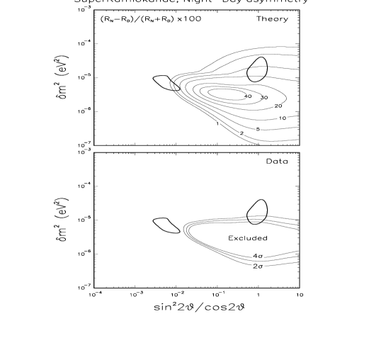
Figure 5: Constraint on the MSW solutions as derived by the measured value of the asymmetry of nihttime ($R_{N}$) and daytime ($R_{D}$) event rates. Upper panel: theoretical expectations for $(R_{N}-R_{D})/(R_{N}+R_{D})$. Lower panel: Regions excluded at 2, 3 and 4 standard deviations by the SUPERKAMIOKANDE data. (From Ref. [41].)

In the prophetical paper of 1946 [8] Bruno Pontecorvo wrote: “direct proof of the existence of the neutrino … must be based on experiments the interpretation of which does not require the law of conservation of energy, i.e. on experiments in which some characteristic process produced by free neutrinos … is observed”.

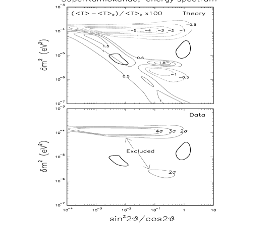
Figure 6: Constraints on the MSW solutions as derived by the measured value of the average electron kinetic energy $<T>$. Upper panel: theoretical expectations for the fractional shifts of $<T>$from its standard (no oscillation) value $<T>_{o}$.Lower panel: region excluded at 2, 3, and 4 standard deviations by SUPERKAMIOKANDE determination of $<T>$. (From Ref. [41].)

The situation now looks very similar, just change existence with non standard properties, in that the strongest argument for a particle physics solution to the SNP arises from energy conservation (the luminosity constraint) and actually we need a direct footprint of some neutrino property, not predicted within the minimal standard model of electroweak interactions.

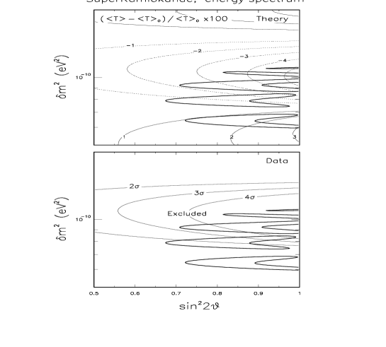
Figure 7: Constraints on the vacuum oscillation solutions as derived by the measured value of the average electron kinetic energy $<T>$. Upper panel: theoretical expectations for the fractional shifts of $<T>$ from its standard (no oscillation) value $<T>_{o}$. Lower panel: region excluded at 2, 3, and 4 standard deviations by SUPERKAMIOKANDE determination of $<T>$. (From Ref. [41].)

The four most popular particle physics solutions (small and large angle MSW effect, just so oscillations and universal oscillations) all predict specific signatures which are being or will be tested by the new generation of experiments (Superkamiokande, Borexino, SNO…), see Table 4.

The universal oscillation solution particularly substained by Perkins et al.  [42] ($\Delta m^{2}\approx 10^{-2}$ eV² and threefold maximal mixing) might account for both the KAMIOKANDE atmospheric neutrino anomaly and the results of solar neutrino experiments (possibly with some stretching of error bars).

This hypothesis has just been falsified by the recent negative result of CHOOZ [43]. This nice and small (in comparison with the gigantic solar neutrino devices) experiment at a nuclear reactor is cleaning some of the fog in the air.

The large angle MSW solution ($\Delta m^{2}\approx 10^{-5}$ eV², twofold maximal mixing) is being under the attack of SUPERKAMIOKANDE [41]. The absence so far of a day-night modulation

$$\frac{N-D}{N+D}=0.017\pm 0.026\,{\mbox{(stat.)}}\,\pm 0.017\,{\mbox{(syst.)}}$$ (15)

clearly excludes a significant portion of the parameter space for this solution, see Fig. 5 and Ref. [41]. On the other hand, the electron spectrum deformations are very small [44, 41], see Fig. 6, and hardly detectable with SUPERKAMIOKANDE.

The small angle MSW solution ($\Delta m^{2}\approx 10^{-5}$ eV², $sen^{2}2\theta\approx 10^{-(2\div 3)}$) is perhaps the most elusive one. As shown in Figs. 5 and 6 both day-night effect and spectrum deformations are very tiny and can escape to SUPERKAMIOKANDE. Possibly, the only detectable signature in future esperiments is in the ratio of Charged Current to Nuclear Current events (CC/NC), see below.

The Just So solution ($\Delta m^{2}\approx 10^{-10}$ eV² and maximal mixing) implies spectral deformation which can be detected with SUPEKAMIOKANDE (see Fig. 7) and seasonal modulations of the ⁷Be signal which will be the realm of BOREXINO [45, 46].

The SNO experiment [47] looks to us, in many respect, as the final remedy/last hope. SNO will be capable of detecting neutral current events, which are produced by any active neutrino. The measurement of the active neutrino flux ($\Phi_{e}+\Phi_{\mu}$) in the ⁸B energy region, combined with the SUPERKAMIOKANDE information ($\Phi_{e}+1/7\,\Phi_{\mu}$), and/or with the charghed current signal of SNO ($\Phi_{e}$), can provide a define proof of neutrino oscillation.

This holds for any of the proposed solutions, unless nature decides that $\nu_{e}$ convert into sterile neutrinos.

Let us wait and wish that (at least) one of the fingerprints of neutrino oscillations is detected by the new experiments.

References

References

- [1] V. Castellani, S. Degl’Innocenti, G. Fiorentini, M. Lissia and B. Ricci, Phys. Rep. 281 (1997) 309.
- [2] J. N. Bahcall, Neutrino Astrophysics, Cambridge University Press, Cambridge, 1989.
- [3] M. Koshiba, Phys. Rep. 220 (1992) 229.
- [4] Kamiokande Collaboration, Phys. Rev. Lett. 77 (1996) 1683.
- [5] SuperKamiokande Collaboration, TAUP97, Laboratori Nazionali del Gran Sasso, September 1997 to appear on Nucl. Phys. B (Proc. Suppl.)
- [6] J.N. Bahcall and M.H. Pinsonneault, Rev. Mod. Phys. 67 (1995) 781.
- [7] B.T. Cleveland, Neutrino 96, Helsinki, June 1996. to appear on Nucl. Phys. B (Proc. Suppl.)
- [8] B. Pontecorvo, Chalk River Report, PD 205 (1946).
- [9] Gallex Collaboration, TAUP97, Laboratori Nazionali del Gran Sasso September 1997. to appear on Nucl. Phys. B (Proc. Suppl.)
- [10] Sage Collaboration, Neutrino 96, Helsinki June 1996 to appear on Nucl Phys. B (Proc. Suppl.)
- [11] GALLEX Collaboration, Phys. Lett. B 342 (1995) 440.
- [12] V. Castellani, S. Degl’Innocenti and G. Fiorentini, Astr. Astroph. 271 (1993) 601.
- [13] V. Castellani, S. Degl’Innocenti, G. Fiorentini, M. Lissia and B. Ricci, Phys. Rev. D 50 (1994) 4749.
- [14] S. Degl’Innocenti, G. Fiorentini and M. Lissia, Nucl. Phys. B (Proc. Suppl.) 43 (1995) 67.
- [15] N. Hata, Solar Modeling, A.B. Balantekin and J.N. Bahcall eds., World Scientific, Singapore 1995.
- [16] N. Hata, S. A. Bludman and P. Langacker, Phys. Rev. D 49 (1994) 3622.
- [17] E. Calabresu, G. Fiorentini, M. Lissia and B. Ricci, Nucl. Phys.. B. (Proc. Suppl.) 48 (1996) 343.
- [18] A. Dar and G. Shaviv, Ap. J. 468 (1996) 933.
- [19] C. R. Proffit, Ap. J. 425 (1994) 849
- [20] O. Richard, S. Vauclair, C. Charbonnel and W. A. Dziembowski, Astron. Astrophys. 312 (1996) 1000.
- [21] F. Ciacio, S. Degl’Innocenti and B. Ricci, Astr. Astroph. Suppl. Series 123 (1997) 1.
- [22] S. Turck-Chieze and I. Lopes, Ap. J. 408 (1993) 347.
- [23] J. N. Bahcall, Phy. Lett. B 338 (1994) 276.
- [24] V. Castellani, S. Degl’Innocenti, G. Fiorentini, M. Lissia and B. Ricci, Phys. Lett. B 324 (1994) 425.
- [25] J. N. Bahcall and A. Ulmer, Phys. Rev. D 53 (1996) 4802.
- [26] V. Berezinsky, Comm. Nucl. Part. Phys. 21 (1994) 249.
- [27] S. Degl’Innnocenti, W.A. Dziembowski , G. Fiorentini and B. Ricci, Astrop. Phys. 7 (1997) 77.
- [28] S. Degl’Innocenti, G. Fiorentini and B. Ricci, astro-ph/9707133, to appear on Phys. Lett. B (1998).
- [29] S. Degl’Innocenti and B. Ricci, astro-ph/9710292, 1997, to appear on Astr. Phys. (1998)
- [30] K.G. Libbrecht, M.F. Woodard and J.M. Kaufman, Ap. J. Suppl. 74 (1990) 1129. F.P. Pijpers and M.J. Thompson,Astron. Astr. 262 (1992) L33.
- [31] Y. Elsworth, R. Howe, G. Isaak and C.P. McLeod, R. New, Ap. J. 434, (1994) 801.
- [32] S. Tomczyk, K. Streander, G. Card, D. Elmore, H. Hull and A. Cacciani, Sol. Phys. 159 (1995) 1.
- [33] J.E. Harvey et al., Science 272 (1996) 1284.
- [34] J. Christensen-Dalsgaard, Nucl. Phys. B (Proc. Suppl.) 48 (1996) 325.
- [35] J. Christensen-Dalsgaard, D.O. Gough and M.J. Thompson Ap. J. 378 (1991) 413.
- [36] W.A. Dziembowski, Bull. Astr. Soc. India 24 (1996) 133.
- [37] J. Christensen-Dalsgaard et al.., Science 272 (1996) 1286.
- [38] J. N. Bahcall, M. H. Pinsonneault, S. Basu and J. Christensen-Dalsgaard, Phys. Rev. Lett. 78 (1997) 171.
- [39] B. Ricci, V. Berezinsky, S. Degl’Innocenti, W.A. Dziembowski and G. Fiorentini, Phys. Lett. B 407 (1997) 155.
- [40] F. Hammache et al., nucl-ex/9712003, to appear on Phys. Rev. Lett. (1998).
- [41] G.L. Fogli, E. Lisi and D. Montanino, hep-ph/9709473
- [42] P.F. Harrison, D.H. Perkins and W.G. Scott, Phys. Lett. B 349 (1995) 137.
- [43] M. Apollonio et al., hep-ex/9711002.
- [44] G. Fiorentini, M. Lissia, G. Mezzorani, M. Moretti and D. Vignaud, Phys. Rev. D 49 (1994) 6298.
- [45] C. Arpesella et al., “Borexino at Gran Sasso: proposal for a real time detector for low energy solar neutrinos”, internal report INFN, Milano, 1992. C. Arpesella et al., Nucl. Phys. B (Proc. Suppl.) 48 (1996) 375.
- [46] E. Calabresu, N. Ferrari, G. Fiorentini and M. Lissia, Astrop. Phys. 4 (1995) 159.
- [47] G. Ewang, Nucl. Instr. and Meth. A 314 (1992) 373.