Obscuration of Quasars by
Dust and the Reddening Mechanism in Parkes-Quasars

by
Franco John Masci

A thesis submitted in total fulfillment of the requirements
for the degree of Doctor of Philosophy

September 1997

School of Physics
The University of Melbourne

I dedicate this thesis to my mother,
whose love and support has made everything possible

Declaration

I hereby declare that my thesis entitled ‘Obscuration of Quasars by Dust and the Reddening Mechanism in Parkes-Quasars’ is the result of my own work and contains nothing which is the outcome of work done in collaboration, with the exception of certain observations. Where work by others has been used, appropriate acknowledgement and references are given. This thesis is not substantially the same, as a whole or in part, as anything I have submitted for a degree or diploma or any other qualification at any other University.

This thesis is less than 100,000 words in length, exclusive of figures, tables, appendices and bibliographies.

Franco J. Masci

Acknowledgements

What a pleasure it is to wake up on this beautiful Spring Melbourne day with a finished thesis, and the thoughts of all those people who have made it possible.

Firstly, I thank my official supervisor, Rachel Webster and my unofficial supervisor, Paul Francis for their enthusiasm and guidance throughout the last four years. I feel I have been very lucky to have had two supervisors both of whom have been generous with their time and ideas. I owe an enormous debt of gratitude to Rachel Webster who has taught me the benefits of a careful and rigorous approach to research. I thank her for shortening my sentences and dealing with all those administrative issues in the University. I extend my warmest thanks to her for everything she has done for me.

Paul Francis’ contribution to this thesis has been incalculable. He displayed enormous patience in teaching me the techniques of observing and data reduction with IRAF. I also thank him for his seemingly boundless knowledge of statistics. I wish to say grazie molto.

This work has benefited enormously from many conversations, long and short, both with numerous visitors to the department and at various conferences and meetings. I wish to extend a special thanks to Michael Drinkwater, Dick Hunstead, Bev Wills, Anne Kinney, Loredana Bassani, Bill Priedhorsky, Bruce Peterson, Kurt Liffman and Vic Kowalenko.

I am also indebted to the graduate students of ‘Room 359’ (the ‘Astro Room’) for discussions and suggestions which only rarely were concerned with the field of astrophysics. Thanks in particular for all the chess games and all the help with my computer-related traumas and spelling dilemmas. I wish you all a prosperous future. A warm thanks to our school librarian Kamala Lekamge for her patience and gratitude. I specially thank Maurizio Toscano and Mathew Britton for lifting my spirits with the finest of Melbourne’s cuisine.

A special thanks to various members of the Melbourne University Mountaineering Club for rejuvenating my academic life with numerous expeditions, far and close, and for sharing my appreciation of the natural environment.

I would particularly like to thank my mother for her tremendous love and support throughout my entire scholastic life. Given the hardships faced following the passing away of my father in 1977, my academic position would not of been possible without her enormous help. I thank her wholeheartedly for making my life possible – grazie molto e non ti dimentico mai. I also thank my brother Kevin and his family for providing constant support and encouragement.

I gratefully acknowledge the University of Melbourne for its financial support.

September 25, 1997

Melbourne

Abstract

A majority of quasar surveys have been based on criteria which assume strong blue continua or a UV-excess. Any amount of dust along the line-of-sight is expected to drastically extinguish the optical/UV flux leading to a selection bias. Radio surveys however should suffer no bias against extinction by dust. Recently, a large complete sample of radio-selected quasars has become available (the ‘Parkes sample’). A majority of these sources exhibit optical–to–near-infrared continua that are exceedingly ‘red’, very unlike those of quasars selected optically. The purpose of this thesis, broadly speaking, is to explore the problem of incompleteness in optical quasar surveys due to obscuration by dust, and to interpret the relatively ‘red’ continua observed in the Parkes quasar sample.

The first part of this thesis explores the observational consequences of an intervening cosmological dust component. A preliminary study explores the effects of different foreground dust distributions (on galaxy-cluster scales to the visible extent of normal galaxies) on obscuration of background sources. Numerical simulations of dusty-galaxies randomly distributed along the line-of-sight with simplified assumptions are then performed, and implications on optical counts of quasars and absorption-line statistics are explored. This foundation is extended by considering the effects of more complicated models of foreground obscuration where the dust content evolves with redshift. The Parkes sample is used to constrain evolutionary and physical properties of dust in intervening systems. The contribution of line-of-sight galactic dust to the reddening observed in this sample is also constrained.

The second part examines the continuum properties of Parkes quasars in the framework of a number of absorption and emission mechanisms to assess the importance of extinction by dust. Three classes of theories are explored: ‘intrinsically red’ AGN emission models, dust extinction models, and host-galaxy light models. Simple models are developed and tested against the available data. Several new correlations between spectral properties are predicted and identified observationally. For the dust model, we explore the effects of dust on soft X-rays and compare our predictions with ROSAT data. Possible physical dust properties are constrained. I then consider the possibility that a ‘red’ stellar component from the host galaxies contributes to the observed reddening. This contribution is quantified using a novel spectral fitting technique. Finally, an observational study of near-infrared polarisation is presented to distinguish between two models for the reddening: the intrinsic ‘synchrotron emission model’, and the dust model. Combined with spectral and photometric data, these observations are used to constrain various emission and dust absorption models.

Preface

Some of my work which has been published, or is due to be published, and that which is not my own, but is extensively used and of substantial importance in this thesis is outlined as follows:

Chapter 1: this chapter involves an introduction and review and thus is not original.

Chapter 2: to be published as Masci & Francis (1997):
Masci,F.J. & Francis,P.J., “Diffuse Dust and Obscuration of the Background Universe.” Publications of the Astronomical Society of Australia, (1997, submitted).
The Cluster-QSO two-point angular correlation data used in section 2.3 is from the literature.

Chapter 3: published as Masci & Webster (1995):
Masci,F.J. & Webster,R.L., “Dust Obscuration in the Universe.” Publications of the Astronomical Society of Australia, 12, p.146 (1995).
The initial stages of the derivation for the probability distribution function in dust optical depth follows from Wright (1986). Except where specifically stated in this and all chapters that follow, all photometric and spectroscopic observations (and their reduction) for the Parkes quasar sample are the result of the following collaborations: Drinkwater $et\,al.$ (1997) and Francis $et\,al.$ (1997).

Chapter 4: to be published as Masci & Webster (1997):
Masci,F.J. & Webster,R.L., “Constraining the Dust Properties of Galaxies Using Background Quasars” (1997, in preparation).
The parameterisation assumed for our evolutionary dust model is partially based on previous indirect studies of the global evolution in heavy metals.

Chapter 5: various aspects of the material presented in section 5.3 was published in Masci & Webster (1996):
Masci,F.J. & Webster,R.L., “Red Blazars”: Evidence Against a Synchrotron Origin. In Proceedings of IAU Conference 163: ‘Accretion Phenomena and Related Outflows.’ ASP Conference Series, 121, p.764 (1996).
The mathematical formalism used to model the synchrotron process (section 5.3.3), and explore diagnostics for X-ray absorption (section 5.6.1) is from the literature. The observational tests presented in sections 5.4.1, 5.5.1 and 5.5.3 were devised in collaboration with Dr. P. Francis, and will appear in Francis $et\,al.$ (1997). Soft X-ray data for Parkes quasars was provided by Siebert $et\,al.$ (1997), and my analysis will appear in Masci $et\,al.$ (1998; in preparation).

Chapter 6: this chapter consists of original research and will be published as Masci & Webster (1998):
Masci,F.J. & Webster,R.L., “Host Galaxy Contribution to the Colours of ‘Red’ Quasars.” Monthly Notices of the Royal Astronomical Society, (1998; submitted).

Chapter 7: Dr. P. Francis assisted generously in the polarimetry observations. A loose description of the reduction procedure was provided by Dr. J. Bailey of which no published material exists. Modelling of the polarimetry data is based on extensions of existing models from a number of independent studies.

Contents

1. Acknowledgements
2. Abstract
3. Preface
4. 1 Introduction
   1. 1.1 Background
      1. 1.1.1 Plan of this Thesis
   2. 1.2 The Study of Cosmic Dust
   3. 1.3 The Interaction of Radiation with Dust and Observational Diagnostics
      1. 1.3.1 Extinction
      2. 1.3.2 Other Diagnostics
   4. 1.4 The Cosmological Distribution of Dust
      1. 1.4.1 Dust in Local Galaxies
      2. 1.4.2 High Redshift Dust and Evolution
   5. 1.5 Dust and Quasars
      1. 1.5.1 Obscuration of Quasars by Intervening Dust
      2. 1.5.2 Dust in the Quasar Environment
      3. 1.5.3 Optically Dust-Obscured Quasars
   6. 1.6 Radio-Selected, Optically Reddened Quasars
5. I Cosmologically Distributed Dust
   1. 2 Diffuse versus Compact Dust Distributions
      1. 2.1 Introduction
      2. 2.2 Compact versus Diffuse Dust Distributions
      3. 2.3 Diffuse Dust in Galaxy Clusters
         1. 2.3.1 Spatial Distribution of Cluster Dust?
         2. 2.3.2 Spatial Distribution of Dust Optical Depth and Background Source Deficits
         3. 2.3.3 Summary
      4. 2.4 Diffuse Intergalactic Dust?
         1. 2.4.1 Comoving Dust Mass Density
         2. 2.4.2 Obscuration by Diffuse Intergalactic Dust
         3. 2.4.3 Summary
      5. 2.5 Discussion
      6. 2.6 Conclusions
   2. 3 Modelling the Obscuration of Quasars by Foreground Dusty Galaxies
      1. 3.1 Introduction
      2. 3.2 Optical Depth Distribution
      3. 3.3 Model Parameters and Results
         1. 3.3.1 Results and Analysis
      4. 3.4 Effect on Quasar Number Counts
         1. 3.4.1 Dust Reddening and Bias in Optically-Selected Samples
      5. 3.5 Comparison with ‘Reddened’ Parkes Quasars
      6. 3.6 Conclusions
   3. 4 Time Evolution of Galactic Dust and the Obscuration of Quasars
      1. 4.1 Introduction
      2. 4.2 The Evolutionary Dust Model
         1. 4.2.1 Evolution
      3. 4.3 Model Parameters and Results
         1. 4.3.1 Model Parameters
         2. 4.3.2 Results and Analysis
      4. 4.4 Implications
         1. 4.4.1 Quasar Absorption Line Systems
         2. 4.4.2 Quasar Evolution and Statistics
      5. 4.5 Constraining Model Parameters
         1. 4.5.1 Observed Reddening Distribution
         2. 4.5.2 Fitting the Data
         3. 4.5.3 Results
      6. 4.6 Comparison With Existing Observations
         1. 4.6.1 Independent Constraints On $\tau_{B}$ and $r_{0}$
         2. 4.6.2 Evolutionary Parameters
      7. 4.7 Discussion
      8. 4.8 Summary and Conclusions
6. II The Reddening Mechanism in Parkes Quasars
   1. 5 The Reddening Mechanism in Parkes Quasars
      1. 5.1 Introduction
         1. 5.1.1 Intrinsically Red Emission Models
         2. 5.1.2 Dust Extinction
      2. 5.2 The Sample
      3. 5.3 The Synchrotron Model
         1. 5.3.1 Radio Core Dominance
         2. 5.3.2 Emission Line Equivalent Widths
         3. 5.3.3 Synchrotron Spectral Shapes
         4. 5.3.4 Summary
      4. 5.4 Other ‘Intrinsically Red’ Emission Models
         1. 5.4.1 ‘Weak’ Optical/UV Emission?
         2. 5.4.2 Emission from Hot Dust
      5. 5.5 Preliminary Tests of the Dust Model
         1. 5.5.1 Emission Line Equivalent Widths
         2. 5.5.2 Optical Continuum Slope versus $B-K$ Colour
         3. 5.5.3 Balmer Decrements
         4. 5.5.4 Summary
      6. 5.6 Soft X-ray Absorption
         1. 5.6.1 Theoretical Investigation
         2. 5.6.2 Analysis of ROSAT Data
         3. 5.6.3 Dust Location: Extrinsic or Intrinsic?
         4. 5.6.4 Summary
      7. 5.7 Implications on Soft X-ray QSO surveys
      8. 5.8 Discussion
         1. 5.8.1 Dust Mass and Thermal Emission?
         2. 5.8.2 Physical Dust Properties
         3. 5.8.3 Further Predictions of the Dust Model
      9. 5.9 Conclusions
   2. 6 Contribution From the Host Galaxy
      1. 6.1 Introduction
      2. 6.2 Preliminary Investigation
      3. 6.3 Outline of Method
         1. 6.3.1 Assumptions
         2. 6.3.2 The Algorithm
         3. 6.3.3 Error Determination
         4. 6.3.4 Summary
      4. 6.4 Data and Input Parameters
         1. 6.4.1 Applying the Algorithm
      5. 6.5 Results
         1. 6.5.1 Spectral Fits
         2. 6.5.2 Systematic vs. Random Errors
         3. 6.5.3 Galactic Contribution to the Observed Optical-Near IR Continuum.
      6. 6.6 A Test for the Unified Model
      7. 6.7 Discussion
      8. 6.8 Conclusions
   3. 7 A Search for Near-Infrared Polarisation
      1. 7.1 Introduction
      2. 7.2 The Observations
         1. 7.2.1 Measuring the Polarisation with IRIS
         2. 7.2.2 Observational Strategy
      3. 7.3 Data Reduction
         1. 7.3.1 Instrumental Effects and Measuring the Polarisation
      4. 7.4 Results
         1. 7.4.1 Polarisation versus Variability and $B-K$ Colour?
      5. 7.5 Origin of the Polarisation?
         1. 7.5.1 Polarisation from Dust
         2. 7.5.2 Polarisation from the Synchrotron Mechanism
      6. 7.6 The Two Component Model: Fits to Observations
         1. 7.6.1 Model Assumptions
         2. 7.6.2 Model Fits and Results
         3. 7.6.3 Summary
      7. 7.7 Discussion
         1. 7.7.1 Further Predictions
      8. 7.8 Conclusions
   4. 8 Conclusions and Future Prospects
      1. 8.1 Conclusions
         1. 8.1.1 Part I: Cosmologically Distributed Dust
         2. 8.1.2 Part II: The Reddening Mechanism in Parkes Quasars
      2. 8.2 Further Work and Future Prospects
         1. 8.2.1 Intervening Cosmological Dust
         2. 8.2.2 Dust Geometry and Location in the Quasar Environment
         3. 8.2.3 Some Theoretical Considerations
         4. 8.2.4 Reddened Radio-Quiet quasars?
      3. 8.3 Summary
   5. A References
   6. B Cosmology
   7. C Derivations in Evolutionary Dust Model

List of Figures

1. 1.1 Extinction curves of the Milky Way, LMC, and SMC
2. 1.2 Observed $B-K$ colour as a function of redshift
3. 2.1 Dependence of background source deficit on radial dust extent
4. 2.2 Extinction by a ‘rich’ galactic cluster
5. 3.1 Optical depth probability distribution functions
6. 3.2 Probability that $\tau_{dust}>1$ as a function of redshift
7. 3.3 Mean optical depth as a function of redshift
8. 3.4 QSO fraction missing from a flux-limited sample vs. $z$
9. 3.5 “True” vs. “Observed” mean optical depth as a function of $z$
10. 4.1 “Observed” optical depth through a single model absorber
11. 4.2 Optical depth probability distribution functions in evolutionary model
12. 4.3 Mean optical depth as a function of $z$ in evolutionary model
13. 4.4 Variance in optical depth as a function of redshift
14. 4.5 Predicted equivalent width distribution and incompleteness in metal absorption line studies
15. 4.6 Comoving number density of quasars with $M_{B}<-26$ as a function of redshift
16. 4.7 Evolutionary model fit to mean reddening of Parkes quasars
17. 4.8 Observed and predicted relative metallicity vs. redshift
18. 5.1 Distribution of $B_{J}-K_{n}$ and optical continuum slope
19. 5.2 $B_{J}-K_{n}$ colour as a function of radio-core dominance
20. 5.3 Prediction for $B-K$ vs. equivalent width in the synchrotron model
21. 5.4 Observed emission line equivalent widths as a function of $B-K$
22. 5.5 Comparisons with the monoenergetic synchrotron model
23. 5.6 Prediction for $B-K$ vs. equivalent width in the ‘weak blue-bump’ model
24. 5.7 Optical spectral slope as a function of near-IR–to–optical continuum slope
25. 5.8 Observed Balmer decrements as a function of optical slope
26. 5.9 X-ray attenuation as a function of observed energy
27. 5.10 Observed and predicted relations between continuum slopes involving the soft X-ray band
28. 5.11 Observed versus predicted 4400Å-to-1keV spectral slope
29. 5.12 QSO fraction lost in soft X-rays due to intrinsic absorption
30. 6.1 Hubble diagram for radio-loud galaxies and Parkes sources
31. 6.2 Composite spectrum of spatially extended Parkes sources
32. 6.3 Spectral evolution of a 1Gyr burst model
33. 6.4 Definition of our “figure of merit” $A$
34. 6.5 Examples of our figure of merit function $A$
35. 6.6 Observed and reconstructed model spectra
36. 6.7 Fractional galaxy contributions for different model assumptions
37. 6.8 Distribution of $1\sigma$ random errors in the fractional galaxy contribution
38. 6.9 Distribution in fractional galaxy contributions in $B_{J}$ and $K_{n}$
39. 6.10 Galaxy contribution in resolved and unresolved sources
40. 6.11 Galaxy contribution to observed $B_{J}-K_{n}$ colours
41. 6.12 Host galaxy $K$ magnitude as a function of redshift
42. 7.1 Schematic of the components of the polarisation vector
43. 7.2 Setup of optical components in the IRIS polarimeter
44. 7.3 Vectorial representation of polarimetric images
45. 7.4 Observed wavelength dependence of percentage polarisation and total flux spectra
46. 7.5 $K_{n}$ polarisation versus variability in $K_{n}$ flux
47. 7.6 $K_{n}$-band polarisation as a function of $B_{J}-K_{n}$ colour
48. 7.7 Predicted wavelength dependence of polarisation from dust
49. 7.8 Predicted polarisation in the monoenergetic synchrotron model
50. 7.9 Polarisation vs. wavelength for a simple two-component model
51. 7.10 Model fits to polarisation and total flux spectra
52. 8.1 Schematic showing possible locations of the dusty medium

List of Tables

1. 3.1 Adopted model parameters for calculation of the distribution functions $p(\tau|z)$.
2. 4.1 Best fit parameters with $1\sigma$ and $2\sigma$ ranges
3. 5.1 Contemporaneous photometry for red quasars and BL-Lacs
4. 7.1 Summary of observations
5. 7.2 Properties of sources in polarimetry study
6. 7.3 Contemporaneous photometry of sources in polarimetry study
7. 7.4 Polarimetry results
8. 7.5 Observed and dust model predictions for polarisation in three ‘moderately reddened’ quasars
9. 7.6 Parameter fits for the ‘two-component model’

Chapter 1 Introduction

“Undoubtedly one of the greatest difficulties, if not the greatest of all, in the way of obtaining an understanding of the real distribution of the stars in space, lies in our uncertainty about the amount of loss suffered by the light on its way to the observer.”

— Jacobus Cornelius Kapteyn, 1909

1.1 Background

Quasars are the most luminous and exotic objects known in the universe and are the only objects observable in large numbers at sizeable redshifts. The most distant quasars known at present have redshifts of $\sim 5$, corresponding to epochs at which the universe was less than 10% of its present age. The standard model (Lynden-Bell, 1969) of a possible supermassive ($\sim 10^{8}M_{\odot}$) black hole fueled by an accretion disk, provides a laboratory for studying the physical processes of matter under extreme conditions.

Quasars are of great importance in astronomy. The fact that they can be seen at early epochs in the universe provides constraints on models for galaxy formation and evolution of the large scale structure. Recently, Katz $et\,al.$ (1994) have shown that the inferred quasar number density at high redshifts can be easily accommodated in hierarchical galaxy formation theories such as CDM in which galaxies form first followed by larger scale structures. As shown by Loeb (1993), the existence of quasars at high redshift implies rapid collapse and very efficient cooling of high mass, dark matter haloes to form black holes on relatively short timescales of $\raisebox{-3.01385pt}{\mbox{$\stackrel{{\scriptstyle\textstyle<}}{{\sim}}$}}1$Gyr.

High redshift quasars provide background light sources to probe the nature and matter content of the intervening medium. This has been achieved through two means. First, the existence of galaxies, proto-galaxies and gas clouds absorb the light from background quasars giving rise to absorption-line features in quasar spectra. Absorption-line studies have provided important constraints on a wealth of physical parameters, including evolution of the neutral hydrogen content in the universe. Second, gravitational lensing of background quasars where light is deflected by intervening matter, can be used to probe mass concentrations in galaxies, haloes and on galaxy cluster scales. Quasars therefore remain an important tool in cosmology for examining the distribution and evolutionary history of matter in the universe.

Despite recent attempts for improving selection techniques for finding quasa- rs, a majority of quasar surveys have been based on criteria which assume strong blue continua or a UV-excess (eg. Schmidt & Green, 1983). Such surveys however are believed to be seriously incomplete as indicated by the increasing numbers of quasars being discovered in X-ray and radio surveys (see Crampton, 1991 for a review). Optical studies are biased against quasars with weak optical continuum emission. Strong evidence for a population of optically-weak quasars has recently been provided by optical follow-up observations of complete radio-selected samples (eg. Kollgaard $et\,al.$ 1995 and references therein; Webster $et\,al.$ 1995). A significant proportion of these sources also have optical continuum slopes much redder than those quasars selected by standard optical techniques. We hypothesise that the most probable explanation is reddening by dust (Webster $et\,al.$ 1995).

Any given amount of dust along the line-of-sight is expected to drastically extinguish the observed UV-optical flux leading to a selection bias. Such dust may be located in the local quasar environment, somewhere along the line-of-sight; for example in intervening dusty galaxies, or a combination of both. If a majority of quasars are obscured by line-of-sight dust, say in intervening galaxies, then studies which use bright optical quasars to detect absorption lines and gravitational lens systems will have underestimated their true abundance. Therefore, an understanding of the effects of dust on quasars is essential. Whatever the mechanism for the optical reddening, if the bulk of quasars remain undetected, then all statistical studies of evolution in the early universe may be seriously incomplete.

In this thesis, I will explore two issues: the problem of incompleteness in optical quasar surveys due to obscuration by dust, and the interpretation of the relatively red optical continua observed in a complete sample of radio quasars (the ‘Parkes sample’). The amount of dust involved, both along the line-of-sight and in the quasar environs is investigated. A number of predictions of the dust reddening hypothesis for Parkes quasars are presented and compared with observations. A more specific outline of the thesis follows.

1.1.1 Plan of this Thesis

This thesis is divided into two parts. Part I (Chapters 2, 3 and 4) is concerned with the observational consequences of an intervening cosmological dust component and uses the Parkes sample to constrain the amount of dust involved. Chapter 2 explores the dependence of the spatial extent of foreground dust distributions on obscuration of background sources. We show that ‘large-scale’ diffusely distributed dust (eg. on galaxy cluster scales) is more effective at obscuring background sources than dust confined to the visible extent of normal galaxies. In Chapter 3, we simulate obscuration by dust located in galaxies randomly distributed along the line-of-sight. We use a range of parameters that may describe the dust properties of galaxies to explore implications on optical counts of quasars. In Chapter 4, we explore the effects of more complicated models of dusty line-of-sight galaxies where the dust content evolves. Implications on quasar and absorption-line statistics are investigated. We use the Parkes sample to constrain evolutionary and physical properties of dust in intervening systems. The contribution of line-of-sight galactic dust to the reddening observed in this sample is quantified.

Part II (Chapters 5, 6 and 7) examines the continuum properties of Parkes quasars in the framework of a number of absorption and emission mechanisms to assess the importance of extinction by dust. Chapter 5 explores two classes of theories to explain the reddening observed: ‘intrinsically red’ AGN emission models, and dust extinction models. Simple models are developed and tested against the available data. For the dust model, we explore the effects of dust on soft X-rays and compare our predictions with soft X-ray data for Parkes sources. Possible physical dust properties are also discussed. In Chapter 6, we consider the possibility that a ‘red’ stellar component from the host galaxies of Parkes quasars contributes to the observed reddening. We quantify this contribution using a new, unbiased spectral fitting method. In Chapter 7, we present a near-infrared polarisation study of Parkes quasars to distinguish between two models for the reddening: the synchrotron emission model and the dust model. Combined with spectral and photometric data, the observations are used to constrain various emission and dust absorption models.

All key results are summarised in Chapter 8. Some avenues for further research suggested from my work on Parkes quasars is also discussed.

1.2 The Study of Cosmic Dust

The first indications that photometric observations of astronomical objects were affected by dust date back to the 1930s when stellar observations by Trumpler (1930) and Stebbins $et\,al.$ (1934) showed that distant parts of the galaxy were obscured by interstellar dust. Since then, observations have established that dust is an important constituent of galaxies. Its presence has significantly contributed to our understanding of star formation rates and on the evolution of galaxy populations with cosmic time (Franceschini $et\,al.$ 1994; De Zotti $et\,al.$ 1995). Recent observations of local galaxies that are suspected of having intense regions of star formation are also observed to be very dusty (see Rieke & Lebofsky, 1979 for a review). Dust is crucial in star forming regions in that it strongly absorbs the UV radiation responsible for molecular dissociations and provides the site for the formation of $\rm{H_{2}}$ - the most abundant molecule in star forming clouds. Dust also controls the temperature of the interstellar medium (ISM). The initial cooling of dense molecular clouds through dust-gas interactions enhances gravitational collapse allowing star formation to occur.

The main questions about dust refer generally to its composition, grain size and temperature. Our knowledge primarily comes from observations of the ISM of our Galaxy and simulations in the laboratory. The grains forming cosmic dust consist of silicates, graphite, dirty ices and heavy metals and range in size from $0.005$-$1\mu$m (Draine, 1981). Grains typical of the ISM of our galaxy form from the condensation of heavy elements initially synthesised in supernovae and grow by accretion in dense molecular clouds, depending crucially on the environment in the ISM. Grains are expected to be efficiently destroyed by supernova shocks in the ISM of galaxies (McKee $et\,al.$ 1987). Recently however, studies have shown that molecular star forming clouds can supply the total ISM dust in less than $10^{8}$ years, at a rate faster than it is destroyed by supernovae (Wang, 1991a and references therein).

Dust absorbs the UV-optical radiation in star-forming regions and re-radiates absorbed energy in the far-infrared part of the spectrum ($10\mu$m-1mm). Observations by the Infrared Astronomy Satellite (IRAS) have shown that radiation by dust from galaxies is comparable to what we see in the visual band (Soifer, Houck & Neugebauer, 1986). Since dust in mostly made of heavy elements, its evolution is directly connected to chemical evolution in the ISM of galaxies. Consequently, observations at infrared wavelengths have contributed significantly towards our understanding of the evolutionary properties of galaxies and their contribution to the integrated background radiation (Wang 1991a; 1991b).

1.3 The Interaction of Radiation with Dust and Observational Diagnostics

The two major processes in which dust grains can alter the transmission of electromagnetic radiation are absorption and scattering. These effects, collectively referred to as extinction, are the best studied property of cosmic dust since they can be accurately determined over a range of wavelengths. A determination of the extinction properties are essential for correcting astronomical measurements for the effects of dust. Other very important diagnostics of dust are its emission properties, both in spectral features and continuum emission in the infrared, and its polarisation properties. These properties are briefly discussed below. An excellent and thorough analysis of the physics can be found in Hoyle & Wickramasinghe (1991).

1.3.1 Extinction

Extinction of radiation at optical wavelengths by dust is largely due to scattering, with the effects of absorption becoming important at shorter wavelengths. Light from a source shining through dust along the line-of-sight has its flux reduced according to

$$F_{\lambda}\,=\,F_{\lambda 0}e^{-\tau_{\lambda}},$$ (1.1)

where $F_{\lambda 0}$ is the flux that would be received at Earth in the absence of dust, $F_{\lambda}$ is the actual flux observed and $\tau_{\lambda}$ is defined as the optical depth at the wavelength observed. This is derived by solving the radiative transfer equation for a homogeneous slab of dust. The extinction in magnitudes is related to the optical depth by $A_{\lambda}=2.5\log(F_{\lambda}/F_{\lambda 0})\equiv 1.086\tau_{\lambda}$. The extinction law is defined by specified values of $\tau_{\lambda}$ at a range of wavelengths and can generally be expressed as

$$\tau_{\lambda}\,=\,C\,f(\lambda),$$ (1.2)

where $C$ relates to the amount of dust and the function $f(\lambda)$ depends on the optical properties of grains.

Extinction laws in our galaxy are primarily determined from observations of stars by comparing the spectral energy distribution of a reddened star with that of an unreddened star of similar spectral-type. The galactic interstellar extinction laws of Savage & Mathis (1979) and Seaton (1979) are commonly used to model the effects of dust and correct astronomical observations. Pei (1992) has obtained excellent empirical fits for extinction curves derived from previous studies for the Milky Way, LMC and SMC. These are shown in Fig. 1.1, where the extinction is measured relative to that observed in the $B$-band, ie. $\xi(\lambda)=\tau_{\lambda}/\tau_{B}$. The striking feature is the almost universal behaviour at wavelengths $\lambda>2500$Å . The “mean” interstellar extinction curve derived in our galaxy varies by a factor of $\sim 10$ in extinction over the range $1000{\rm\AA}<\lambda<2\mu$m and exhibits both continuous extinction and a strong feature known as the “2175Å  bump” over which the extinction varies appreciably. This feature decreases in strength going from the Milky Way to the LMC and SMC. This bump is believed to be due to graphite, however its origin is not as yet well understood.

Figure 1.1: Empirical fits to the extinction curves of the Milky Way, LMC, and SMC from Pei (1992). The extinction $\xi$ is measured relative to that observed in the $B$-band ($\equiv\tau_{\lambda}/\tau_{B}$). Also shown (dashed) is the extinction law derived by Calzetti $et\,al.$ (1994) for external galaxies.

It is remarkable that a recent study by Calzetti $et\,al.$ (1994) finds no evidence for a 2175Å  bump feature in the extinction curves of nearby galaxies (see dashed curve in Fig. 1.1). These authors also find the extinction laws for a number of galaxies to be considerably flatter as a function of wavelength in the UV, with extinction measures smaller by factors of $\raisebox{-3.01385pt}{\mbox{$\stackrel{{\scriptstyle\textstyle>}}{{\sim}}$}}3$ at $\lambda\raisebox{-3.01385pt}{\mbox{$\stackrel{{\scriptstyle\textstyle<}}{{\sim}}$}}1590$Å  than those in the Milky Way. This behaviour is commonly referred to as “gray extinction”. They attribute the “grayness” as being due to their method of derivation. Their method relies on examining correlations between the Balmer line ratio ($H\alpha/H\beta$; see section 5.5.3) and optical continuum reddening. Each of these quantities is expected to arise from different physical regions in the galaxies: the hydrogen lines from hot ionizing stars associated with dusty regions, and the continuum from older stellar populations which may have had time to drift away from the dustier regions. Thus, the continuum measurements may be weighted mostly by regions of lowest extinction. The absence of the 2175Å  bump feature has been interpreted as being either due to effects of scattering of light within extended dust-regions into the line-of-sight (therefore reducing the effective extinction in the UV), or to a chemical composition of grains different from that in the Milky Way.

There have been many efforts devoted to the understanding of the composition and optical properties of dust grains giving rise to the various extinction laws, in particular that of the Milky Way (Mathis, Rumpl & Nordsiek, 1977; Drain & Lee, 1984). These authors have studied different chemical mixtures to reproduce the Milky Way extinction law and as yet no definite agreement exists. Draine & Lee (1984) find that for a $1:1.12$ graphite and silicate mixture, the extinction (or the function $f(\lambda)$ in Eqn. 1.2) at optical wavelengths varies as a function of wavelength as $f(\lambda)=\lambda^{-n}$, where $n\sim 1$-2. This is derived using the optical properties of grains and the theory of light scattering which involves a solution of Maxwell’s equations. The index $n$ depends on the characteristic grain size “$a$”, and its dependence has been studied via the extinction efficiencies $Q_{ext}(a,\lambda)$ of spherical dielectric grains (eg. Greenberg, 1968). In the optical–to–near-infrared, the extinction law in our galaxy approaches the characteristic behaviour $\lambda^{-1}$. This is expected when the sizes of individual grains become comparable with the wavelength of light ($\lambda\sim a$), where the extinction efficiency is given by $Q_{ext}\propto\lambda^{-1}$. For comparison, when the grain sizes are very small compared with the wavelength ($a\ll\lambda$), the extinction efficiency varies as $Q_{ext}\propto\lambda^{-4}$, known as the Rayleigh scattering regime. When $a\gg\lambda$, $Q_{ext}$ levels off asymptotically to about twice the geometric cross-section of the grain. Hence, larger grain sizes produce a flatter dependence with wavelength.

Approaching higher energies such as X-rays, and depending on the grain size, grains become somewhat transparent. Using graphite and silicate mixtures, Laor & Draine (1993) show that the extinction decreases by at least two orders of magnitude from 0.1-10keV (see Fig. 5.9). At energies $\raisebox{-3.01385pt}{\mbox{$\stackrel{{\scriptstyle\textstyle>}}{{\sim}}$}}1$keV, the dust extinction law becomes the same as if all grains were composed of neutral atoms in the gas phase rather than possibly being ionized. In this case, atomic X-ray absorption will dominate the optical depth. At soft energies ($\raisebox{-3.01385pt}{\mbox{$\stackrel{{\scriptstyle\textstyle<}}{{\sim}}$}}0.5$keV), the X-ray absorption cross-section is dominated mostly by H and He which, given a large neutral fraction, can attenuate the X-ray flux by more than 80%, even for relatively low values of the hydrogen column density (ie. $N_{H}\raisebox{-3.01385pt}{\mbox{$\stackrel{{\scriptstyle\textstyle>}}{{\sim}}$}}10^{18}{\rm cm}^{-2}$). At $\raisebox{-3.01385pt}{\mbox{$\stackrel{{\scriptstyle\textstyle>}}{{\sim}}$}}1$keV however, absorption becomes dominated by metals (primarily the K-edges of oxygen and carbon and to a lesser extent Ne, Mg, Si, S and Fe - Morrison & McCammon, 1983). See section 5.6.1 for more details. Metals in dust grains can be shielded from the effects of X-ray absorption, however, modifications of only a few percent to their absorption cross-section are expected, even at soft X-ray energies (Fireman, 1974).

1.3.2 Other Diagnostics

In addition to general extinction over a continuous wavelength range, the presence of spectral absorption features can be used to confirm the presence of dust, and also provide information regarding the compositions and nature of the grains. Apart from the 2175Å  bump in our galaxy, strong $9.7\mu$m and $18\mu$m absorption/emission features are almost always seen in our ISM and the ISM of a number of external galaxies when the dust is optically thin to its own emission, ie. $\tau_{10\mu{\rm m}}\ll 1$. These features have been attributed to silicate grains with sizes $a\raisebox{-3.01385pt}{\mbox{$\stackrel{{\scriptstyle\textstyle<}}{{\sim}}$}}3\mu$m (Laor & Draine, 1993). These authors also show that their absence in the near-infrared spectra of active galaxies (including luminous quasars) provides important constraints on the chemical and physical properties of dust in such sources (see section 1.5.2 for more details).

Infrared (IR) continuum emission from dust grains can arise through two means. First, by absorption and heating by UV photons and subsequent re-radiation at infrared wavelengths and second, by steady state emission or fluorescence. The latter process occurs for far-infrared wavelengths, $\lambda>100\mu$m. An important diagnostic of this emission is in the determination of dust temperatures and/or masses. These can be calculated by assuming that dust grains are in thermal equilibrium with their surroundings so that the emission can be approximated as a blackbody. The blackbody radiation law can be written

$$B(\nu,T_{d})\,=\,\frac{2h\nu^{3}}{c^{2}}\frac{1}{\exp(h\nu/kT_{d})-1}\,\,\,{\rm erg\,cm^{-2}sec^{-1}Hz^{-1}ster^{-1}}.$$ (1.3)

Given measurements of the infrared flux at two or more frequencies, the dust temperature $T_{d}$ can be determined by fitting equation 1.3. In the determination of dust masses however, we define an additional quantity called the dust emissivity, $\kappa_{\nu}$, with units ${\rm cm^{2}}$ per gram of dust. From galactic observations at sub-mm wavelengths, $\kappa_{\nu}\propto\nu^{2}$ (Chini & Krügel, 1994). As an example, let us consider an IR-source at some redshift $z$, whose observed IR flux is due to thermal dust emission. The dust mass, assuming the dust is optically thin to its own emission with effective temperature $T_{d}$ is given by

$$M_{dust}=\frac{S_{\nu_{o}}D_{L}^{2}}{(1+z)\kappa_{\nu_{r}}B(\nu_{r},T_{d})},$$ (1.4)

where $\nu_{o}$ and $\nu_{r}$ are the observed and rest frame frequencies respectively, $\kappa_{\nu_{r}}$ is the dust emissivity defined above, $D_{L}$ the luminosity distance and $S_{\nu_{o}}$ the observed flux. The factor $(1+z)$ is due to the decrease in frequency bandpass in the observer’s frame with increasing redshift. Depending on the temperature $T_{d}$ and emission frequency $\nu$, there are two limiting behaviours for the blackbody radiation law (Eqn. 1.3) which are commonly used to simplify calculations. One limit is the well known Rayleigh-Jean’s law and is applicable in the low frequency limit:

$$B(\nu,T_{d})\,\approx\,2\left(\frac{\nu}{c}\right)^{2}kT_{d}\,{\rm\hskip 28.45274ptfor\hskip 5.69054pt}\,\frac{h\nu}{kT_{d}}\ll 1.$$ (1.5)

In the high frequency limit, we have Wien’s law:

$$B(\nu,T_{d})\,\approx\,\frac{2h\nu^{3}}{c^{2}}\exp\left(-\frac{h\nu}{kT_{d}}\right)\,{\rm\hskip 28.45274ptfor\hskip 5.69054pt}\,\frac{h\nu}{kT_{d}}\gg 1.$$ (1.6)

As a general rule, the blackbody law allows us to approximate the effective dust temperature through the relation:

$$T_{d}\,\simeq\,2898\left(\frac{\lambda_{max}}{\mu{\rm m}}\right)^{-1}{\rm K},$$ (1.7)

where $\lambda_{max}$ is the wavelength at which the emission peaks (ie. where $B(\nu,T_{d})$ is a maximum). If dust is to survive, it is estimated that grains cannot exceed a temperature of $\sim 1500$K after which evaporation or sublimation will occur. Thus, we expect dust to emit only at wavelengths $\lambda\raisebox{-3.01385pt}{\mbox{$\stackrel{{\scriptstyle\textstyle>}}{{\sim}}$}}2\mu$m. Evidence for hot dust approaching the limiting temperature $T_{d}\sim 1500$K is believed to exist in the environments of quasars and other active galaxies, giving rise to the characteristic near-IR bump observed in the range $1-3\mu$m (Sanders $et\,al.$ 1989).

Polarisation of radiation produced by scattering or transmission through aligned dust particles provides a useful diagnostic for determining the size distribution of dust grains, the conditions under which grains can be aligned (eg. magnetic field geometry) and most importantly, the geometry of scattering regions (Whittet, 1992 and references therein). In the Milky Way, where the most accurate determinations of dust-polarisation have been made, the polarisation is of order a few percent. The polarisation properties of dust are less well determined than those of extinction, however, optical polarisation coincident with extinction or IR emission may confirm that the latter processes are due to dust.

To summarise, the difficulties in drawing a consistent picture of the interaction of dust grains with radiation lie in their chemical and physical properties, such as composition and grain size distribution. These properties, which are primarily determined from extinction measures, are very sensitive to the geometrical distribution of dust in galaxies and hence subject to considerable uncertainty.

1.4 The Cosmological Distribution of Dust

Infrared and optical studies of local galaxies have provided a good description of their dust content, however, the study of dust at high redshift has yet to produce conclusive results. Despite many efforts for detecting high redshift ($z>1$) galaxies in the optical, it is suspected that large numbers are obscured by dust associated with intense star formation activity (Djorgovski $et\,al.$ 1993; Franceschini, 1994). Our knowledge regarding high redshift dust (at $z>2$) has primarily come from two sources. First, by direct imaging of intrinsically luminous, high redshift radio galaxies at far-IR to mm wavelengths, and second, from studies of QSO absorption line systems. The observational status is given below.

1.4.1 Dust in Local Galaxies

Various morphological and spectral studies of nearby galaxies have demonstrated that the bulk of their IR luminosity originates from extended emission by dust. The local far-infrared luminosity density is estimated to be about one-third of the optical luminosity density (eg. Saunders $et\,al.$ 1990). This emission has lead to estimates of galactic dust masses in the range $10^{7}$-$10^{9}M_{\odot}$, ie. $\raisebox{-3.01385pt}{\mbox{$\stackrel{{\scriptstyle\textstyle<}}{{\sim}}$}}0.5\%$ of the total mass in a typical galaxy (Rieke & Lebofsky, 1979). Furthermore, Zaritsky (1994a) has provided strong evidence for diffuse dust haloes extending to distances $\sim 60h_{75}^{-1}$ kpc from the centers of galaxies. This was provided by studies of the colours of distant galaxies seen through the haloes of nearby spirals, where background galaxies at smaller projected separations were statistically redder than those in outer regions. If such a diffuse component proves to be common, then the local dust content is expected to be greater by almost an order of magnitude than previously estimated using IR emission alone.

In cases where IR emission is not observed, measures of the dust optical depth using surface photometry can provide a useful diagnostic for determining the dust content of galaxies. This method is based on statistical studies of the dependence of optical surface brightness on the viewing angle of a spiral disk. For a transparent disk, the surface brightness depends sensitively on inclination, while for an opaque “dusty” disk it does not (Holmberg, 1958). This allows limits to be placed on the dust optical depth. One caveat however is that this method is limited to galaxies of relatively high surface brightness. Recent studies predict central $B$-band optical depths for spiral galaxies in the range $0.5\raisebox{-3.01385pt}{\mbox{$\stackrel{{\scriptstyle\textstyle<}}{{\sim}}$}}\tau_{B}\raisebox{-3.01385pt}{\mbox{$\stackrel{{\scriptstyle\textstyle<}}{{\sim}}$}}2$ (Giovanelli $et\,al.$ 1994 and references therein). In E/SO galaxies, extinction is not as well studied, though not believed to be as large. Goudfrooij $et\,al.$ (1994a; 1994b; 1995) suggest there is a diffuse component with $0.1\raisebox{-3.01385pt}{\mbox{$\stackrel{{\scriptstyle\textstyle<}}{{\sim}}$}}\tau_{B}\raisebox{-3.01385pt}{\mbox{$\stackrel{{\scriptstyle\textstyle<}}{{\sim}}$}}0.9$. These optical depth properties still remain an open question.

1.4.2 High Redshift Dust and Evolution

Luminous radio galaxies can be studied out to large cosmological distances. Recently, a number of radio galaxies at redshifts $z\raisebox{-3.01385pt}{\mbox{$\stackrel{{\scriptstyle\textstyle>}}{{\sim}}$}}3$ have been observed to emit a strong far-IR to mm continuum. If the emission is assumed to be thermal emission from dust, then dust masses comparable to those of local galaxies are implied (Chini & Krügel, 1994 and references therein). The detection of dusty objects at $z\sim 4$ is puzzling. One might expect that the majority of objects at high redshifts (corresponding to epochs only $5-10\%$ of the age of the universe) still contain a large reservoir of primordial gas. The presence of dust implies an early episode of star formation and provides a step towards understanding the interstellar medium, and hence formation and evolution of galaxies at high redshift.

Strong evidence for the existence of dust at high redshift is provided by studies of QSO absorption line systems. The highest neutral hydrogen column density systems known as the damped Ly-$\alpha$ absorbers are believed to be the progenitors of present day galactic disks. Observations of trace metals such as Ni, Cr and Zn in these systems have provided an opportunity to study chemical and dust evolution in galaxies at high redshift (Meyer & Roth, 1990; Pettini $et\,al.$ 1994; 1997).

The relative strengths of various metal ions in the spectra of background quasars have been used to infer the amount of metal depletion in the gas phase and hence the amount of dust assuming depletion onto grains. Recent studies of metal absorption line systems towards redshifts $z\sim 2$ have indicated metallicities which are $\sim 10\%$ solar and dust-to-gas ratios less than $8\%$ of the galactic value (Meyer, Welty and York, 1989; Pettini $et\,al.$ 1994). This constraint on the dust-to-gas ratio is also in agreement with studies by Fall $et\,al.$ (1989) who compared the spectra of quasars that have damped Ly-$\alpha$ with those that do not. They found that quasars with damped Ly-$\alpha$ absorption in their spectra had spectral slopes somewhat redder than those without absorption.

The lower metal abundances in QSO absorption systems relative to those in the galaxy have been interpreted as evidence for less chemical enrichment at high $z$. It is important to note however that such measurements may be subject to considerable observational bias. Existing observations of QSOs with damped Ly-$\alpha$ absorption lines are drawn mostly from optically-selected, magnitude-limited samples and hence, it is possible than an unrecognised population of highly reddened QSOs may escape detection due to heavy obscuration by dust in damped Ly-$\alpha$ systems. Thus, present QSO absorption line studies may only preferentially pick out chemically unevolved gas. Fall & Pei (1993) have attempted to correct for this bias, estimating that the true metal and dust content may be on average 2-3 times greater than that deduced observationally.

There seems to be considerable difficulty in applying the results of QSO absorption line studies and high redshift radio galaxy surveys to the study of primeval galaxies and evolution of their ISM. It may be some time before large enough, complete statistical samples can be compiled so to obtain a consistent picture of chemical and dust evolution in the universe. At present, we must resort to dynamical modelling of stellar processes in galaxies to gain some insight into this problem (eg. Wang 1991a and references therein).

1.5 Dust and Quasars

In my study of the effects of dust on the properties and identification of quasars in the optical, I shall investigate two possibilities for its location. First, I will consider extrinsic or line-of-sight dust associated with foreground galaxies and second, intrinsic dust or dust physically associated with the quasars themselves. A brief review of the status on each of these studies is given below.

1.5.1 Obscuration of Quasars by Intervening Dust

Studies investigating the effects of intervening, cosmologically distributed dust on background quasars were initially motivated by the apparent lack of high redshift quasars in the optical (McKee & Petrosian, 1974; Cheney & Rowan-Robinson, 1981). Based on observations of individual quasar spectra, colours and counts as a function of redshift, it was concluded that uniformly distributed intergalactic dust as distinct from galactic dust was not likely to be a large source of extinction. From thereon, modelling of this problem assumed all dust to be situated in clumps or hypothesised dusty galaxies along the line-of-sight.

Various theoretical studies by Ostriker & Heisler (1984); Heisler & Ostriker (1988), Fall & Pei (1989, 1993) and Wright (1986, 1990) conclude that at least $70\%$ of bright quasars at redshifts $z\raisebox{-3.01385pt}{\mbox{$\stackrel{{\scriptstyle\textstyle>}}{{\sim}}$}}3$ may be obscured by intervening galactic dust in the optical. A more refined treatment was undertaken by Wright (1990) who stressed the importance of galaxy “hardness” on the properties of a quasar sample subject to both flux and colour selection effects. The term “hardness” depends on the assumed spatial distribution for dust optical depth through an individual galaxy. For optical depth profiles which are smooth or “fuzzy” around the edges (eg. an exponential or King model), the “hardness” is defined by the magnitude of the central optical depth. For central $B$-band optical depths $\tau_{B}\gg 1$, galaxies were defined as being “hard-edged” up to a typical scale radius, while for $\tau_{B}\raisebox{-3.01385pt}{\mbox{$\stackrel{{\scriptstyle\textstyle<}}{{\sim}}$}}1$, galaxies were defined as “soft-edged”. For “sharp-edged” optical depth profiles (eg. an optical depth which is uniform throughout a finite projected area and zero outside - as considered by Ostriker & Heisler, 1984), the hardness is defined by the magnitude of this optical depth. Wright (1990) found that galaxies which are “soft” around the edges will cause many background quasars to ‘appear’ reddened without actually removing them from a flux-limited sample.

It is important to note that these studies are extremely model dependent. The most crucial parameters are the number of absorbing galaxies involved and their dust properties (eg. individual optical depths and dust spatial extent). These parameters are presently known to within a factor of three. Further studies to determine these parameters are therefore necessary before plausible conclusions regarding the effects of foreground dust on optical observations of high redshift quasars can be made.

If published estimates of the effects of foreground dust on optical studies of quasars are correct, then implications for present cosmological studies are immense. Studies which use bright optical quasars to count absorption line systems and gravitational lenses may have severely underestimated their true abundance. Studies involving damped Ly-$\alpha$ absorption systems to determine a wealth of physical parameters such as chemical composition, dust and gas content, and star formation rates at high redshift, are also likely to be affected (Fall & Pei, 1993; Pei & Fall, 1995). If substantial numbers of quasars remain undetected, then a significant fraction of the observed $\gamma$- and X-ray background may arise from dust obscured quasars (Heisler & Ostriker, 1988). More importantly, these quasars would significantly contribute to the UV photon density at high redshifts, thereby altering the nature and physical state of the intergalactic medium at early epochs.

1.5.2 Dust in the Quasar Environment

There are two major lines of study investigating the existence and properties of dust in the neighbourhood of quasars. The first class of studies is based on the observed IR emission. It is suggested that the near-IR “bump” at $1-3\mu$m and spectral turnover at $\lambda>100\mu$m in a majority of optically-selected quasars can be attributed to emission by dust (Neugebauer $et\,al.$ 1979; McAlary & Rieke, 1988; Sanders $et\,al.$ 1989). In fact, about a third of the total luminosity from quasars is emitted in the $1-100\mu$m range (Sanders $et\,al.$ 1989). The most attractive explanation for this emission is thermal radiation from dust heated by a central UV-optical continuum source. This is supported by a significant lack of variability and polarisation in the IR compared to the emission properties at $\lambda<1\mu$m (Sitko & Zhu, 1991). The IR continuum emission can be fitted with a variety of models: optically thin dust in a spherical distribution (Barvainis, 1987), optically thick dust in a torus with equatorial optical depths $A_{V}\sim 100$ on scales less than a few hundred parsecs (Pier & Krolik, 1992), or dust in a highly warped disk on much larger scales (Sanders $et\,al.$ 1989). These studies are consistent with a significant number of quasars having their optical emission substantially reduced, preventing their detection in the optical.

The second class of studies involve searching for dust from differential extinction of emission lines in the optical-UV spectra of quasars (Draine & Bahcall, 1981; MacAlpine, 1985; Netzer & Laor, 1993). MacAlpine (1985) and Netzer & Laor (1993) conclude that much of the absorbing dust is likely to be embedded within the narrow line emitting gas (the NLR) on scales no larger than about a kiloparsec, ie. on scales a little larger than that of a possible dusty torus. Dust in the NLR is expected to modify the physical conditions of the emitting gas and consequently, the continuum spectral slope (see MacAlpine, 1985 for a review).

Together with studies of the IR continuum, these studies have provided strong constraints on the possible location for dust in quasars and other lower luminosity active galactic nuclei (AGN). For quasars, it is predicted that dust grains are heated to high evaporation temperatures. Barvainis (1987) has estimated an “evaporation radius” greater than $\sim 1$pc, ie. scales much larger than the hypothesised broad line emitting region (BLR). Furthermore, the characteristic turnover at $\lambda\sim 100\mu$m has been shown to imply that a significant fraction of the thermal IR radiation may be emitted from scales $\raisebox{-3.01385pt}{\mbox{$\stackrel{{\scriptstyle\textstyle>}}{{\sim}}$}}100$pc (Edelson, Malkan & Rieke, 1987). This leaves two possible options for the location of the dust: a torus and/or NLR clouds, or the quasar host galaxy.

There is remarkable similarity between quasars and other nearby, less luminous AGN such as Seyferts. The growing importance of dust in Seyfert galaxies may suggest that at least some quasars should also exhibit similar properties. Recently, optically thick dust with azimuthal symmetry such as a torus, has been invoked to explain the difference between broad and narrow-line AGN in the framework of unified schemes (Antonucci, 1993). The distribution of this material in a torus can obscure the central UV-optical continuum source and BLR from direct view, while emission from the larger scale NLR is unaffected. This is supported by spectropolarimetric observations showing broad emission lines in polarized light in narrow line (type-II) Seyfert galaxies. Further evidence for a torus-shaped dust region is provided by the observation of ionization cones in several Seyfert galaxies, demonstrating that the gas in the host galaxy sees an anisotropic ionizing source. Evidence for dust tori in high redshift quasars is scarce. However, spectropolarimetric observations revealing the presence of a hidden BLR, combined with a reddened UV-optical continuum has been found in two quasars (Hines & Wills, 1992 and Wills $et\,al.$ 1992).

1.5.3 Optically Dust-Obscured Quasars

One drawback in the above studies investigating “intrinsic” dust, is that almost all are based on optically-selected quasar samples. Optical studies are expected to be heavily biased against significant extinction by dust. These inevitably show that dust is present and an important constituent of quasars, however, it is possible that a large population remains undetected optically due to obscuration by dust. Evidence for such a population may be provided by studies at wavelengths where no bias against dust obscuration is expected. There are three possible wavelength regimes of interest: The infrared, X-rays and the radio. I shall consider each in turn below.

Near or far-infrared surveys may provide a useful means of detecting dust obscured quasars. The ideal strategy is to look for intrinsically luminous point like sources in the IR. Follow-up IR-spectroscopy is then required for further identification of standard characteristics such as broad emission lines. The ultraluminous infrared sources detected by the Infrared Astronomy Satellite (IRAS) are likely candidates for dust-obscured quasars. These sources have IR luminosities comparable to those of quasars ($L_{IR}\raisebox{-3.01385pt}{\mbox{$\stackrel{{\scriptstyle\textstyle>}}{{\sim}}$}}10^{11}L_{\odot}$) and there is debate about whether such objects host buried quasars (Hines $et\,al.$ 1995 and references therein). Evidence for such a population has been presented by Hill $et\,al.$ (1987) and Sanders $et\,al.$ (1988). Moreover, a large abundance of faint, possibly dust-obscured quasars is suggested by the IRAS selected sample of Low $et\,al.$ (1989). In this study, FeII emission was shown to be prominent in quasars with strong IR luminosity relative to their optical emission, suggesting a medium significantly enriched in metals and dust. Through an investigation of their radio properties, Lonsdale $et\,al.$ (1995) claim that it is physically plausible for dust enshrouded quasars to power the IR emission observed from IRAS sources.

X-ray selected samples may provide stronger evidence for an optically obscured quasar population. Soft X-rays ($\raisebox{-3.01385pt}{\mbox{$\stackrel{{\scriptstyle\textstyle<}}{{\sim}}$}}0.5$keV) are subject to considerable absorption by hydrogen and heavy metals (see section 5.6.1), and hence soft X-ray surveys are expected to be heavily biased. Hard X-rays ($\raisebox{-3.01385pt}{\mbox{$\stackrel{{\scriptstyle\textstyle>}}{{\sim}}$}}5$keV) however penetrate the dust, and absorption may become significant only when the gas column density is sufficiently high, ie. $\raisebox{-3.01385pt}{\mbox{$\stackrel{{\scriptstyle\textstyle>}}{{\sim}}$}}10^{23}{\rm cm}^{-2}$ (Awaki $et\,al.$ 1990). Stocke $et\,al.$ (1991) found a factor of almost two orders of magnitude dispersion in the X-ray-to-optical ratios of an X-ray selected sample as compared to those selected optically. This scatter may be caused by variable dust extinction in the optical and in fact supports the claim by McDowell $et\,al.$ (1989) for a possible a correlation between X-ray-to-optical flux ratio and $B-K$ colour.

There have been numerous X-ray spectroscopic studies claiming soft X-ray absorption in excess of that expected from the galaxy in the spectra of radio-selected quasars (Madejski $et\,al.$ 1991; Wilkes $et\,al.$ 1992; Elvis $et\,al.$ 1994). Absorptions corresponding to $\raisebox{-3.01385pt}{\mbox{$\stackrel{{\scriptstyle\textstyle>}}{{\sim}}$}}10^{22}$ atoms ${\rm cm}^{-2}$ were deduced in a majority of cases. These studies however failed to detect any associated extinction by dust in the optical. A correlation is expected at some level, however as will be discussed in section 5.6.1, these separate processes may critically depend on the physical conditions, locations and geometry of the absorbing gas and dust.

Optical identification of radio-selected sources probably provides the best technique for detecting dust-obscured quasars, being subject to fewer possible selection effects than surveys based at X-ray or IR wavelengths. Criteria for selecting quasars in the radio is primarily based on their characteristic “flat” spectral energy distribution at GHz frequencies; $\alpha\raisebox{-3.01385pt}{\mbox{$\stackrel{{\scriptstyle\textstyle<}}{{\sim}}$}}0.5$ where $S_{\nu}\propto\nu^{-\alpha}$. Most of the bright (ie. $\raisebox{-3.01385pt}{\mbox{$\stackrel{{\scriptstyle\textstyle>}}{{\sim}}$}}0.1$Jy) radio surveys based on this criterion have $\raisebox{-3.01385pt}{\mbox{$\stackrel{{\scriptstyle\textstyle>}}{{\sim}}$}}70\%$ of sources identified with quasars which have optical properties extremely similar to those selected optically. More than 10% also comprise sources which are highly polarised and strongly variable at radio to optical wavelengths. These sources belong to the “Blazar” class of AGN (Angel & Stockman, 1980). There have been very few radio-surveys specifically aimed towards finding quasars. Most surveys did not include criteria based on radio spectral-slope. Both steep and flat-spectrum sources were selected, where the former comprised the majority of sources and were usually identified with galaxies. For instance, an optical study of a complete radio sample with $S_{2.7{\rm GHz}}>0.1$Jy by Dunlop $et\,al.$ (1989) found a quasar fraction $\raisebox{-3.01385pt}{\mbox{$\stackrel{{\scriptstyle\textstyle<}}{{\sim}}$}}30\%$. Their spectroscopic identifications however are also significantly incomplete.

Recently, the largest and most complete radio-selected quasar sample has been compiled by Drinkwater $et\,al.$ (1997), initially selected from the Parkes Catalogue. All sources have flat radio spectra ($\alpha<0.5$) and 2.7GHz fluxes $S>0.5$Jy at the epoch of the Parkes survey. Based on a high identification rate in the optical and near-infrared, this study may provide crucial evidence for a substantial population of dust-reddened quasars. A broad and flat distribution in optical–to–near-IR colour with $2\leq B-K\leq 10$ as compared to $B-K\sim 2-3$ for an optically selected sample was found (see Fig. 1.2). It is important to note however that only $\sim 10\%$ of sources in optical-quasar surveys are radio-loud. It is uncertain then whether the distribution of reddening in this sample is applicable to samples of radio-quiet QSOs. If so, then this sample predicts that existing optical quasar-samples may be only $\sim 20\%$ complete (Webster $et\,al.$ 1995).

Figure 1.2: Distribution in $B_{J}-K$ colour as a function of redshift for quasars from a complete sample of radio-loud, flat spectrum sources (filled circles; Drinkwater $et\,al.$ 1996), and a subsample of optically selected quasars from the Large Bright Quasar Survey (LBQS-open circles; Hewett $et\,al.$ 1995). Sources with unknown redshifts are shown at right.

1.6 Radio-Selected, Optically Reddened Quasars

Radio-selected quasars have optical characteristics very similar to those selected optically. Recent studies however have found one exception: as seen from Fig. 1.2, the large spread in optical–near-IR colour suggests that not all quasars can be characterised by the lower envelope cutoff of $B-K\sim 2.5$. This section gives a brief review of the previous work aimed at disentangling the nature of this “red” population.

In previous studies, flat-spectrum radio sources where no optical counterpart was detected were often classified as “Empty Fields”. Deep optical and near-infrared observations in fact showed that many were very red in optical–near-IR colour. They were characterised by spectral indices, $\alpha\raisebox{-3.01385pt}{\mbox{$\stackrel{{\scriptstyle\textstyle>}}{{\sim}}$}}2$, where $S_{\nu}\propto\nu^{-\alpha}$ (Spinrad & Smith, 1975; Rieke, Lebofsky & Kinman, 1979; Bregman $et\,al.$ 1981; Rieke $et\,al.$ 1982). For comparison, optically-selected quasars (see Fig. 1.2) are characterised by optical–near-IR spectral indices $\sim 0.2-0.3$.

Possible causes for the relatively red optical–to–near-IR continua have been discussed, but no consensus exists. Some authors have claimed that since a majority of these flat-spectrum radio sources were also associated with “blazar-like” activity, the redness may be a characteristic of the synchrotron emission mechanism. (Cruz-Gonzalez & Huchra 1984; Bregman $et\,al.$ 1981; Rieke $et\,al.$ 1982). Other explanations such as optical continuum reddening by dust somewhere along the line-of-sight have been suggested, but evidence has been scarce. Some of the observational tests (eg. Ledden & O’Dell, 1983) included searching for metal absorption-line systems, X-ray absorption, or effects of gravitational lensing if the absorbing material lies in an unrelated intervening system. In a study by Ledden & O’Dell (1983) and more recently by Kollgaard $et\,al.$ (1995), evidence for soft X-ray absorption was presented for a few of the reddest sources. The numbers however were too low to draw any firm conclusion.

The difficulty in obtaining a self-consistent picture of radio-loud optically reddened quasars lies in the lack of sufficient knowledge of the sources themselves. There appear to be no additional characteristics which correlate with optical reddening that may provide a hint about the physics.

More than 40% of the 323 sources in the complete, flat spectrum radio sample of Drinkwater $et\,al.$ (1997) have optical–near-IR colours $B-K\,\raisebox{-3.01385pt}{\mbox{$\stackrel{{\scriptstyle\textstyle>}}{{\sim}}$}}\,5$. This corresponds to optical–near-IR spectral indices $\alpha\,\raisebox{-3.01385pt}{\mbox{$\stackrel{{\scriptstyle\textstyle>}}{{\sim}}$}}\,1.8$, very much redder than those of optically selected quasars where $\alpha\sim 0.2-0.3$. At present, it remains unclear whether these sources represent one extreme of the flat spectrum radio population or a fundamentally new class of AGN. Their faint identifications and red colours suggest that significant numbers of quasars may be severely under-represented in current optical surveys. The last chapters of this thesis shall explore possible physical mechanisms to explain the anomalous properties of sources in this sample.

Part I Cosmologically Distributed Dust

Chapter 2 Diffuse versus Compact Dust Distributions

Who can number the clouds by wisdom
Or who can pour out the bottles of heaven,
When the dust runneth into a mass,
And the clods cleave fast together?

— Job, 38:37

2.1 Introduction

There are number of studies claiming that dust in foreground galaxies has a substantial effect on the colours and counts of optically selected quasars (Ostriker & Heisler, 1984; Heisler & Ostriker, 1988; Fall & Pei, 1992 and Wright, 1990). It is estimated that more than 50% of bright quasars at a redshift of $z\sim 3$ may be obscured by dust in intervening galaxies and hence missing from optical samples. These studies assumed that dust was confined only within the visible extent of normal massive galaxies. However, distant populations such as faint field galaxies and quasars may also be observed through foreground diffuse dust distributions. Such distributions may be associated with galaxy clusters and extended galactic haloes.

A truly diffuse, intergalactic dust distribution is ruled out based on the counts of quasars and reddening as a function of redshift (eg. Rudnicki, 1986; Ostriker & Heisler, 1984). Such observations indicate that if a significant amount of dust exists, it must be patchy and diffuse with relatively low optical depth so that quasars will appear reddened without being removed from flux limited samples.

Galaxy clusters provide a likely location for ‘large-scale’ diffusely distributed dust. Indirect evidence is provided by several studies which reported large deficits of distant quasars or clusters of galaxies behind nearby clusters (Boyle $et\,al.$ 1988; Romani & Maoz, 1992 and references therein). These studies propose that extinction by intracluster dust is the major cause. Additional evidence for diffuse dust distributions is provided by observations of massive local galaxies where in a few cases, dust haloes extending to scales $\raisebox{-3.01385pt}{\mbox{$\stackrel{{\scriptstyle\textstyle>}}{{\sim}}$}}50$kpc have been confirmed (Zaritsky, 1994 and Peletier $et\,al.$ 1995; see the review in section 1.4.1).

It is possible that a uniformly distributed dust component exists in the intergalactic medium (IGM). Galactic winds associated with prodigious star formation activity at early epochs may have provided a likely source of metal enrichment and hence dust for the IGM (eg. Nath & Trentham, 1997). Observations of metal lines in Ly$\alpha$ absorption systems of low column density ($N_{HI}\raisebox{-3.01385pt}{\mbox{$\stackrel{{\scriptstyle\textstyle<}}{{\sim}}$}}10^{15}{\rm cm^{-2}}$) indeed suggest that the IGM was enriched to about $Z\sim 0.01Z_{\odot}$ by redshift $z\sim 3$ (Womble $et\,al.$ 1996; Songaila & Cowie, 1996). A source of diffuse dust may also have been provided by an early generation of pre-galactic stars (ie. population III stars) associated with the formation of galactic haloes (McDowell, 1986). Later in this thesis, it will be shown that possible reddening from uniformly distributed IGM dust is limited by observations of radio-selected quasars. Since radio-selected quasars should have no bias against reddening by dust (see section 1.5.3), such a component must be of sufficiently low optical depth to avoid producing a large fraction of ‘reddened’ sources at high redshift (see Fig. 1.2).

In this chapter, we show that a given quantity of dust has a much greater effect on the background universe when diffusely distributed. We shall investigate the effects of diffuse dust from, firstly, the existence of a diffuse component in galaxy clusters and secondly, from a hypothesised uniformly distributed component in the IGM.

This chapter is organised as follows: in the next section, we explore the dependence of background source counts observed through a given mass of dust on its spatial extent. In section 2.3, we investigate the spatial distribution of dust optical depth through galaxy clusters and its effect on the counts and colours of background sources. Section 2.4 explores the consequences if all dust in the local universe were assumed uniformly distributed in the IGM. Further implications are discussed in section 2.5 and all results are summarised in section 2.6. All calculations use a Friedmann cosmology with $q_{0}=0.5$ and Hubble parameter $h_{50}=1$ where $H_{0}=50h_{50}\,\rm km\,s^{-1}\,Mpc^{-1}$.

2.2 Compact versus Diffuse Dust Distributions

In this section, we explore the dependence of obscuration of background sources on the spatial distribution of a given mass of dust. For simplicity, we assume the dust to be associated with a cylindrical face-on disk with uniform spatial dust mass density. We quantify the amount of obscuration by investigating the number of background sources behind our absorber that are missed from an optical flux-limited sample.

The fraction of sources missing to some luminosity $L$ relative to the case where there is no dust extinction is simply $1-N_{obs}(>L)/N_{true}(>L)$, where $N_{obs}(>L)$ represents the observed number of sources in the presence of dust. For a uniform dust optical depth $\tau$, $N_{obs}(>L)\equiv N_{true}(>e^{\tau}L)$. For simplicity, we assume that background sources are described by a cumulative luminosity function that follows a power-law: $\Phi\propto L^{-\beta}$, where $\beta$ is the slope. With this assumption, the fraction of background sources missing over a given area when viewed through our dusty absorber with uniform optical depth $\tau$ is given by

$$f_{miss}(\tau)\,=1\,-\,e^{-\beta\tau}.$$ (2.1)

If the ‘true’ number of background sources per unit solid angle is $n_{true}$, then the total number of background sources lost from a flux limited sample within the projected radius $R$ of our absorber can be written:

$$N_{lost}(\tau)\,=\,n_{true}\frac{\pi R^{2}}{D^{2}}(1\,-\,e^{-\beta\tau}),$$ (2.2)

where $D$ is the distance of the absorber from us.

To investigate the dependence of background source counts on the spatial dust distribution, we need to first determine the dependence of $\tau$ in Eqn. 2.2 on the spatial extent $R$ for a fixed mass of dust $M_{d}$. This can be determined from the individual properties of grains as follows. The extinction optical depth at a wavelength $\lambda$ through a slab of dust composed of grains with uniform radius $a$ is defined as

$$\tau_{\lambda}\,=\,Q_{ext}(\lambda,a)\pi a^{2}n_{d}l_{d},$$ (2.3)

where $Q_{ext}$ is the extinction efficiency which depends on the grain size and dielectric properties, $n_{d}$ is the number density of grains and $l_{d}$ is the length of the dust column along the line-of-sight. Assuming our cylindrical absorber (whose axis lies along the line-of-sight) has a uniform dust mass density: $\rho_{dust}=M_{d}/\pi R^{2}l_{d}$, where $R$ is its cross-sectional radius, we can write, $n_{d}=\rho_{dust}/\frac{4}{3}\pi a^{3}\rho_{d}$, where $\rho_{d}$ is the mass density of an individual grain. We use the extinction efficiency $Q_{ext}$ in the $V$-band as parameterised by Goudfrooij $et\,al.$ (1994) for a graphite and silicate mixture (of equal abundances) with mean grain size $a\sim 0.1\mu$m characteristic of the galactic ISM. The value used is $Q_{ext}(V,0.1\mu m)=1.4$. We use a galactic extinction curve to convert to a $B$-band extinction measure, where typically $\tau_{B}\sim 1.3\tau_{V}$ (eg. Pei, 1992). Combining these quantities, we find that the $B$-band optical depth, $\tau_{B}$, through our model absorber can be written in terms of its dust mass and cross-sectional radius as follows:

$$\tau_{B}\,\simeq\,1\left(\frac{M_{d}}{10^{8}M_{\odot}}\right)\left(\frac{R}{20{\rm kpc}}\right)^{-2}\left(\frac{a}{0.1\mu{\rm m}}\right)^{-1}\left(\frac{\rho_{d}}{2{\rm gm}\,{\rm cm}^{-3}}\right)^{-1},$$ (2.4)

where we have scaled to a dust mass and radius typical of local massive spirals and ellipticals (eg. Zaritsky, 1994). This measure is consistent with mean optical depths derived by other means (eg. Giovanelli $et\,al.$ 1994 and references therein).

From Eqn. 2.4, we see that the dust optical depth through our model absorber for a fixed dust mass varies in terms of its cross-sectional radius $R$ as $\tau\propto 1/R^{2}$. For the nominal dust parameters in Eqn. 2.4, the number of sources missed behind our model absorber (Eqn. 2.2) can be written

$$N_{lost}(<R)\,=\,N_{true}(<20{\rm kpc})\,R_{20}^{2}(1-e^{-\beta R_{20}^{-2}}),$$ (2.5)

where $R_{20}=R/20{\rm kpc}$ and

$$N_{true}(<20{\rm kpc})\,\equiv\,n_{true}\frac{\pi(20{\rm kpc})^{2}}{D^{2}}$$ (2.6)

is the ‘true’ number of background sources falling within the projected scale radius $R=20$kpc.

From the functional forms of Eqns. 2.2 and 2.5, there are two limiting cases:

1. For optical depths $\tau\gg 1/\beta$, the factor $1-e^{-\beta\tau}$ in Eqn. 2.2 is of order unity. This corresponds to values of $R$ such that $0<R_{20}\ll\beta^{1/2}$ for the nominal parameters in Eqn. 2.4. For values of $R$ in this range, we have $N_{lost}\propto R^{2}$ and the obscuration of background sources will depend most strongly on $R$.

2. For $\tau\ll 1/\beta$ or equivalently $R_{20}\gg\beta^{1/2}$, $N_{lost}$ will approach a constant limiting value, independent of the dust extent $R$. From Eqn. 2.5, this limiting value can be shown to be $N_{lost}(<R)\,=\,N_{true}(<20{\rm kpc})\beta$.

As a simple illustration, we show in Fig. 2.1 the dependence of the number of background sources missing behind our model dust absorber on $R$, for a fixed dust mass of $10^{8}M_{\odot}$ as defined by Eqn. 2.5. We assumed a cumulative luminosity function slope of $\beta=2.5$, typical of that for luminous galaxies and quasars. From the above discussion, we see that when $R_{20}\raisebox{-3.01385pt}{\mbox{$\stackrel{{\scriptstyle\textstyle>}}{{\sim}}$}}\beta^{1/2}$, ie. $R\raisebox{-3.01385pt}{\mbox{$\stackrel{{\scriptstyle\textstyle>}}{{\sim}}$}}30{\rm kpc}$ (or when $\tau\raisebox{-3.01385pt}{\mbox{$\stackrel{{\scriptstyle\textstyle<}}{{\sim}}$}}1/\beta=0.4$), the obscuration will start to approach its maximum value and remain approximately constant as $R\rightarrow\infty$.

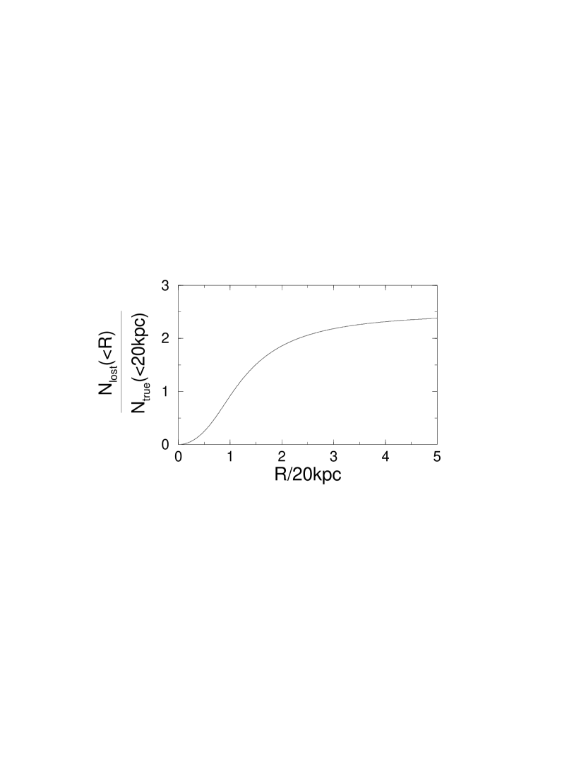
Figure 2.1: The number of sources missing from an optical flux limited sample behind a face-on dusty disk with fixed mass $M_{dust}=10^{8}M_{\odot}$ as a function of its radial extent $R$. This number is normalised against the ‘true’ number of background sources (in the absence of the absorber) that fall within the solid angle $\pi(20{\rm kpc})^{2}/D^{2}$ subtended by our nominal radius of 20kpc at distance $D$. See Eqn. 2.5.

We conclude that when dust becomes diffuse and extended on a scale such that the mean optical depth $\tau$ through the distribution satisfies $\tau<1/\beta$, where $\beta$ is the cumulative luminosity function slope of background sources, obscuration will start to be important and is maximised for $\tau\ll 1/\beta$. The characteristic spatial scale at which this occurs will depend on the dust mass through Eqn. 2.4. For the typical grain values in Eqn. 2.4, this characteristic radius is given by

$$R\,\simeq\,31\left(\frac{\beta}{2.5}\right)^{1/2}\left(\frac{M_{d}}{10^{8}M_{\odot}}\right)^{1/2}{\rm kpc}.$$ (2.7)

The simple model in Fig. 2.1 shows that the obscuration of background sources due to a normal foreground galaxy will be most effective if dust is distributed over a region a few times its optical radius. This prediction may be difficult to confirm observationally due to possible contamination from light in the galactic absorber. In the following sections, we explore two examples of possible diffuse dust distributions on relatively large scales that can be explored observationally.

2.3 Diffuse Dust in Galaxy Clusters

A number of studies have attributed the existence of large deficits of background sources behind nearby galaxy clusters as due to extinction by dust. Bogart & Wagner (1973) found that distant rich Abell clusters were anticorrelated on the sky with nearby ones. They argued for a mean extinction of $A_{V}\approx 0.4$mag extending to $\sim 2.5$ times the optical radii of the nearby clusters. Boyle, Fong & Shanks (1988) however claimed a $\sim 30\%$ deficit of background quasars within $4^{\prime}$ of clusters consisting of tens of galaxies. These authors attribute this to an extinction $A_{V}\approx 0.15$mag, and deduce a dust mass of $\sim 10^{10}M_{\odot}$ within 0.5Mpc of the clusters. Romani & Maoz (1992) found that optically-selected quasars from the Véron-Cetty & Véron (1989) catalogue avoid rich foreground Abell clusters. They also found deficits of $\sim 30\%$ out to radii $\sim 5^{\prime}$ from the clusters, and postulate a mean extinction, $A_{V}\approx 0.4$mag.

The numbers of background sources behind clusters is also expected to be modified by gravitational lensing (GL) by the cluster potential. Depending on the intrinsic luminosity function of the background population, and the limiting magnitude to which the sources are detected, GL can cause either an enhancement or a deficit in the number of background sources. The GL effect has been used to explain various reports of overdensities of both optically and radio-selected quasars behind foreground clusters (Bartelmann & Schneider, 1993; Bartelmann $et\,al.$ 1994; Rodrigues-Williams & Hogan, 1994; Seitz & Schneider, 1995). The reported overdensities for optically-selected QSOs are contrary to the studies above where anticorrelations with foreground clusters are found. These overdensities however are claimed on angular scales $\sim 10^{\prime}-30^{\prime}$ from the cluster centers, considerably larger than scales on which most of the underdensities have been claimed, which are of order a few arcminutes. One interpretation is that dust obscuration bias may be greater towards cluster centers due to the presence of greater quantities of dust. On the other hand, the reported anticorrelations on small angular scales can perhaps be explained by the optically crowded fields, where QSO identification may be difficult. At present, the effects of clusters on background source counts still remains controversial.

More direct evidence for the existence of intracluster dust was provided by Hu $et\,al.$ (1985) and Hu (1992) who compared the Ly-$\alpha$ flux from emission line systems in “cooling flow” clusters with Balmer line fluxes at optical wavelengths. Extinctions of $A_{V}\sim 0.2-1$mag towards the cluster centers were found, in good agreement with estimates from the quasar deficits above. Intracluster dust has been predicted to give rise to detectable diffuse IR emission (eg. Dwek $et\,al.$ 1990). The most extensive search was conducted by Wise $et\,al.$ (1993), who claimed to have detected excess diffuse 60-100$\mu$m emission at the 2$\sigma$ level from a number of rich Abell clusters. They derived dust temperatures in the range 24-34 K and dust masses $\sim 10^{10}M_{\odot}$ within radii of $\sim 1$Mpc. Recently, Allen (1995) detected strong X-ray absorption and optical reddening in ellipticals situated at the centers of rich cooling flow clusters, providing strong evidence for dust. These studies indicate that intracluster dust is certainly present, however, the magnitude of its effect on producing background source deficits remains a controversial issue.

In this section, we give some predictions that may be used to further constrain cluster dust properties, or help determine the dominant mechanism (ie. GL or extinction) by which clusters affect background observations.

2.3.1 Spatial Distribution of Cluster Dust?

X-ray spectral measurements show the presence of hot, metal enriched gas in rich galaxy clusters with $\sim 0.5-1$ solar metallicity. This gas is believed to be both of galactic and primordial origin (ie. pre-existing IGM gas), with the bulk of metals being ejected from cluster galaxies (see Sarazin, 1986 for a review). Ejection from galaxies may occur abruptly through collisions between the cluster galaxies, ‘sudden’ ram-pressure ablation, or through continuous ram-pressure stripping by intracluster gas (eg. Takeda $et\,al.$ 1984). The lack of significant amounts of dust (relative to what should have been produced by stellar evolution) and interstellar gas in cluster ellipticals provides evidence for a mass loss process. On the other hand, in ellipticals that avoid dense cluster environments, significant quantities of neutral hydrogen, molecular gas and dust have been detected (eg. Lees $et\,al.$ 1991).

If the dust-to-gas ratio of intracluster gas in rich clusters were similar to that of the Milky Way, then a radial gas column density of typically $\raisebox{-3.01385pt}{\mbox{$\stackrel{{\scriptstyle\textstyle>}}{{\sim}}$}}10^{22}{\rm cm}^{-2}$ with metallicity $Z=0.5Z_{\odot}$ would produce an extinction $A_{V}\raisebox{-3.01385pt}{\mbox{$\stackrel{{\scriptstyle\textstyle>}}{{\sim}}$}}4$mag. This however is much greater than the value observed. The likely reason for the deficiency of dust in the intracluster medium is its destruction by thermal sputtering in the hot gas, a process which operates on timescales $t_{sputt}\raisebox{-3.01385pt}{\mbox{$\stackrel{{\scriptstyle\textstyle<}}{{\sim}}$}}10^{8}n_{-3}a_{0.1}$ yr, where $n_{-3}=n_{H}/10^{-3}{\rm cm}^{-3}$ is the gas density and $a_{0.1}=a/0.1\mu{\rm m}$ the grain radius (Draine & Salpeter, 1979). Dust injection timescales from galaxies is typically of order a Hubble time (eg. Takeda $et\,al.$ 1984) and hence, grains are effectively destroyed, with only the most recently injected still surviving and providing possibly some measurable extinction.

The spatial distribution in dust mass density remains a major uncertainty. A number of authors have shown that under a steady state of continuous injection from cluster galaxies, destruction by thermal sputtering at a constant rate, and assuming instantaneous mixing with the hot gas, the resulting mass density in dust will be of order

$$\rho_{dust}\,\sim\,10^{-31}\left(\frac{a}{0.1\mu{\rm m}}\right)\left(\frac{Z_{d}}{0.01}\right)h_{50}\,\,{\rm gm}\,{\rm cm}^{-3},$$ (2.8)

(eg. Dwek $et\,al.$ 1990) where $Z_{d}$ is the injected dust-to-gas mass ratio, assumed to be equal to the mean value of the galactic ISM, $Z_{d}\simeq 0.01$ (Pei, 1992). According to this simple model, the dust mass density is independent of gas density and position in the cluster. If we relax the assumption of instantaneous mixing of dust with the hot gas however, so that the spatial distribution of gas is different from that of the injected dust, the radial distribution of dust can significantly differ from uniformity throughout a cluster. Such a non-uniform spatial dust distribution may be found in clusters exhibiting cooling flows. If, as suggested by Fabian $et\,al.$ (1991), most of the cooled gas remains cold and becomes molecular in cluster cores, then a relatively large amount of dust may also form, resulting in a dust distribution which peaks within the central regions.

We explore the radial dependence of extinction optical depth through a cluster, and the expected deficit in background sources by assuming that dust is diffusely distributed and follows a spatial density distribution:

$$\rho_{dust}(R)\,=\,\rho(0)\left[1-\left(\frac{R}{R_{c}}\right)^{2}\right]^{-n},$$ (2.9)

where $R_{c}$ is a characteristic radius which we fix and $n$ is our free parameter. Eqn. 2.9 with $n=3/2$ is the usual King profile which with $R_{c}\simeq 0.25$Mpc, represents a good approximation to the galaxy distribution in clusters. Thus for simplicity, we keep $R_{c}$ fixed at $R_{c}=0.25$Mpc and vary $n$. To bracket the range of possibilities in the distribution of intracluster dust, we shall consider the range $0\,<\,n\,<\,3/2$. $n=0$ corresponds to the simple case where $\rho_{dust}(R)=\rho(0)=$constant, which may describe a situation where injection of dust is balanced by its destruction by hot gas as discussed above. The value $n=3/2$ assumes that dust follows the galaxy distribution. This profile may arise if grain destruction by a similar distribution of hot gas were entirely absent.

2.3.2 Spatial Distribution of Dust Optical Depth and Background Source Deficits

To model the spatial distribution of optical depth, we assume that intracluster dust is distributed within a sphere of radius $R_{max}$. The central dust mass density $\rho(0)$ in Eqn. 2.9 is fixed by assuming values for the total dust mass $M_{dust}$ and $R_{max}$ such that

$$M_{dust}=\int^{R_{max}}_{0}{4\pi R^{2}\rho(R)\,dR}.$$ (2.10)

We assume a cluster dust radius of $R_{max}=1$Mpc, which represents a radius containing $\raisebox{-3.01385pt}{\mbox{$\stackrel{{\scriptstyle\textstyle>}}{{\sim}}$}}90\%$ of the virial mass of a typical dense cluster characterised by galactic velocity dispersion $\sigma_{V}\sim 800{\rm kms}^{-1}$ (Sarazin, 1986 and references therein). We assume that the total dust mass within $R_{max}=1$Mpc is $M_{dust}=10^{10}M_{\odot}$. This value is consistent with that derived from extinction measures by Hu, Cowie & Wang (1985), IR emission detections by Wise $et\,al.$ (1993) and theoretical estimates of the mean intracluster dust density as given by Eqn. 2.8.

Using Eqn. 2.3, the $B$-band optical depth through our spherical intracluster dust distribution at some projected distance $r$ from its center can be written:

$$\tau_{B}(r)\,=\,\frac{3Q_{ext}}{4a\rho_{d}}\int^{2(R_{max}^{2}-r^{2})^{1/2}}_{0}{\rho_{dust}\left([r^{2}+R^{\prime 2}]^{1/2}\right)\,dR^{\prime}},$$ (2.11)

where $\rho_{dust}(R)$ is our assumed radial density distribution (Eqn. 2.9) and $\rho_{d}$ the mass density of an individual dust grain. For a uniform dust density ($\rho_{dust}(R)=\rho_{dust}(0)=$constant), and our assumed values of $R_{max}$ and $M_{dust}$ given above, the radial dependence in dust optical depth can be written:

$$\tau_{B}(r)\,=\,\tau_{B}(0)\left[1-\left(\frac{r}{R_{max}}\right)^{2}\right]^{1/2},$$ (2.12)

where $\tau_{B}(0)$ is the optical depth through the center of our cluster, which with grain properties characteristic of the galactic ISM, will scale as

$$\tau_{B}(0)\,\simeq\,0.06\left(\frac{M_{dust}}{10^{10}M_{\odot}}\right)\left(\frac{R_{max}}{{\rm Mpc}}\right)^{-2}\left(\frac{a}{0.1\mu{\rm m}}\right)^{-1}\left(\frac{\rho_{d}}{2{\rm gm}\,{\rm cm}^{-3}}\right)^{-1}.$$ (2.13)

This value is about a factor three times lower than estimates of the mean extinction derived from the deficit of QSOs behind foreground clusters (eg. Boyle $et\,al.$ 1988), and that implied by the Balmer decrements of Hu $et\,al.$ (1985). For a fixed dust mass of $10^{10}M_{\odot}$ however, we can achieve larger values for the central optical depth by steepening the radial dust-density distribution profile, determined by the slope $n$ in Eqn. 2.9.

Fig. 2.2a shows the optical depth as a function of projected cluster radius for the cases $n=0$, 0.5, 1, and 1.5. The case $n=0.5$ approximately corresponds to the model of Dwek $et\,al.$ (1990), which included effects of mild sputtering by hot gas in order to fit for the observed IR emission from the Coma cluster. As shown, the case $n=0$ ($\rho_{dust}(R)=$constant) predicts that the dust optical depth should be almost independent of projected radius $r$. Within all projected radii, the optical depths predicted by our diffuse dust model lie in the range $0<\tau_{B}<0.3$. Turning back to the discussion of section 2.2 where we show that background obscuration by diffuse dust reaches its maximum for $\tau_{B}<1/\beta$, these optical depths satisfy this condition for $\beta\raisebox{-3.01385pt}{\mbox{$\stackrel{{\scriptstyle\textstyle<}}{{\sim}}$}}2.5$, typical of luminous background galaxies and quasars.

Figure 2.2: a. Optical depth as a function of projected cluster radius for various dust density distributions as parameterised by Eqn. 2.9. b. Differential number of background sources lost from a flux-limited sample (arbitrary scale). c. Total fraction of background sources missing to some $r$ and d. Cluster-QSO two-point angular correlation function, filled circles: Boyle $et\,al.$ (1988), squares: Romain & Maoz (1992), open circles: Rodrigues-Williams & Hogan (1994), triangles: Rodrigues-Williams & Hawkins (1995).

We now explore the effects of these models on background source counts as a function of projected cluster radius. We first give an estimate of the projected radius at which the numbers of background sources lost from a flux-limited sample is expected to be a maximum. This is determined by investigating the dependence in the differential number of sources missing, $dN_{lost}$, within an interval ($r,r+dr$) as a function of projected radius $r$. From Eqn. 2.2, this differential number will scale as

$$dN_{lost}(r)\,\propto\,r\,dr\left[1-e^{-\beta\tau(r)}\right],$$ (2.14)

where $\tau(r)$ is given by Eqn. 2.11. Fig. 2.2b plots $dN_{lost}/dr$ as a function of $r$ for our various models, where we have assumed $\beta=2.5$. Thus from observations, an identification of the projected radius at which the background source deficit peaks can be used to constrain the spatial distribution of intracluster dust.

The cumulative fraction of background sources missing within a projected cluster radius is given by

$$f_{miss}(<r)\,=\,\frac{N_{lost}(<r)}{N_{true}(<r)}\,=\,\frac{1}{\pi r^{2}}\int^{r}_{0}{2\pi r^{\prime}\left[1-e^{-\beta\tau(r^{\prime})}\right]\,dr^{\prime}}.$$ (2.15)

This fraction is shown in Fig. 2.2c. As expected, the $n=3/2$ model which contains the largest amount of dust within the inner few hundred kiloparsecs predicts the strongest trend with $r$, while the opposite is predicted if the dust density were completely uniform. These predictions can be compared with a number of existing studies of the observed two-point angular correlation function between clusters and optically-selected QSOs. This function is usually defined as

$$w_{cq}(\theta)\,=\,\frac{\langle N_{obs}(<\theta)\rangle}{\langle N_{ran}(<\theta)\rangle}\,-\,1,$$ (2.16)

where $\langle N_{obs}(<\theta)\rangle$ is the average number of observed cluster-QSO pairs within an angular radius $\theta$ and $\langle N_{ran}(<\theta)\rangle$ is that expected in a random distribution. For our purposes, $\langle N_{ran}(<\theta)\rangle$ can be replaced by the “true” number of cluster-QSO pairs expected in the absence of dust, and hence, we can re-write Eqn. 2.16 as

$$w_{cq}(\theta)\,\equiv\,-\frac{\langle N_{lost}(<\theta)\rangle}{\langle N_{true}(<\theta)\rangle}\,=\,-f_{miss}(<\theta).$$ (2.17)

We compare our models with a number of studies of $w_{cq}(\theta)$ for optically selected QSOs in Fig. 2.2d. These studies considerably differ from each other in the selection of the QSO and cluster samples, and as seen, both anticorrelations and correlations on different angular scales are found. The former have been interpreted in terms of extinction by intracluster dust, while the latter with the GL phenomenon. In most cases, the reported overdensities are too large to be consistent with GL models given our current knowledge of cluster masses and QSO distributions.

It is interesting to note that the studies which have reached the smallest angular scales ($\raisebox{-3.01385pt}{\mbox{$\stackrel{{\scriptstyle\textstyle<}}{{\sim}}$}}5^{\prime}$) are also those in which anticorrelations between QSOs and foreground clusters have been reported. This can be understood in terms of a larger dust concentration and hence extinction towards cluster centers. These studies however may not be free of selection effects, such as in the detection of QSOs from the visual inspection of objective prism plates. From a cross-correlation analysis of galactic stars with their cluster sample however, Boyle $et\,al.$ (1988) found that such selection effects are minimal.

The maximum dust radial extent assumed in our models, $R_{max}=1$Mpc, corresponds to angular scales $\sim 5^{\prime}$ at the mean redshift of the clusters ($\langle z_{c}\rangle\sim 0.15$) used in these studies. Thus, as shown in Fig. 2.2d, our model predictions only extend to $\sim 5^{\prime}$. As shown in this figure, the $n=3/2$ model which corresponds to the case where the dust density is assumed to follow the galaxy distribution, provides the best fit to the Boyle $et\,al.$ (1988) data. We must note that this is the only existing study performed to angular scales $\sim 1^{\prime}$ with which we can compare our models. Further studies to such scales are necessary to confirm the Boyle $et\,al.$ result, and/or provide a handle on any selection effects.

2.3.3 Summary

To summarise, we have shown that for a plausible value of the dust mass in a typical rich galaxy cluster, obscuration of background sources will be most effective if dust is diffusely distributed on scales $\sim 1$Mpc. This conclusion is based on our predicted optical depths ($\tau_{B}<0.3$) satisfying our condition for ‘maximum’ obscuration: $\tau_{B}<1/\beta$ (see section 2.2), where typically $\beta\raisebox{-3.01385pt}{\mbox{$\stackrel{{\scriptstyle\textstyle<}}{{\sim}}$}}2.5$ for luminous background galaxies and QSOs.

We have explored the spatial distribution in dust optical depth and background source deficits expected through a typical rich cluster by assuming different radial dust density profiles. These predictions can be used to constrain cluster dust properties. A dust density distribution with $n=3/2$ (Eqn. 2.9) appears to best satisfy the ‘small scale’ cluster-QSO angular correlation study of Boyle $et\,al.$ (1988).

2.4 Diffuse Intergalactic Dust?

There have been a number of studies claiming that the bulk of metals in the local universe had already formed by $z\sim 1$ (eg. Lilly & Cowie, 1987; White & Frenk, 1991; Fall & Pei, 1995). Similarly, models of dust evolution in the galaxy show that the bulk of its dust content was formed in the first few billion years (Wang, 1991). These studies suggest that the global star formation rate peaked at epochs $z\raisebox{-3.01385pt}{\mbox{$\stackrel{{\scriptstyle\textstyle>}}{{\sim}}$}}2$ when the bulk of galaxies were believed to have formed. Supernova-driven winds at early epochs may thus have provided an effective mechanism by which chemically enriched material and dust were dispersed into the IGM. As modelled by Babul & Rees (1992), such a mechanism is postulated to be crucial in the evolution of the ‘faint blue’ galaxy population observed to magnitudes $B\sim 28$. Nath & Trentham (1997) also show that this mechanism could explain the recent detection of metallicities $Z\sim 0.01Z_{\odot}$ in low density Ly$\alpha$ absorption systems at $z\sim 3$. Another source of diffuse IGM dust may have been provided from an epoch of population III star formation associated with the formation of galactic haloes (eg. McDowell, 1986).

What are the effects expected on background sources if all dust formed to the present day was completely uniform and diffuse throughout the IGM? In this section, we show that such a component will have a low optical depth and have an insignificant effect on the colours of background sources, but will be high enough to significantly bias their number counts in the optical.

2.4.1 Comoving Dust Mass Density

To explore the effects of a diffuse intergalactic dust component, we need to assume a value for the mean mass density in dust in the local universe. This density must not exceed the total mass density in heavy metals at the present epoch. An upper bound for the local mass density in metals (hence dust) can be derived from the assumption that the mean metallicity of the local universe is typically: $Z\sim\Omega_{metals}/\Omega_{gas}\sim 0.01$ (ie. the ratio of elements heavier than helium to total gas mass), as found from galactic chemical evolution models (eg. Tinsley, 1976) and abundance observations (Grevesse & Anders, 1988). Combining this with the upper bound in the baryon density predicted from big-bang nucleosynthesis (Olive $et\,al.$ 1990) where $\Omega_{gas}\raisebox{-3.01385pt}{\mbox{$\stackrel{{\scriptstyle\textstyle<}}{{\sim}}$}}\Omega_{baryon}<0.06h_{50}^{-2}$, it is apparent that

$$\Omega_{metals}(z=0)\,<\,6\times 10^{-4}h_{50}^{-2}.$$ (2.18)

Let us now compute the total mass density in dust used in previous studies that modelled the effects of dust in individual galaxies on background quasars. Both Heisler & Ostriker (1988) and Fall & Pei (1993) modelled these effects by assuming that dust in each galaxy was distributed as an exponential disk with scale radius $r_{0}\simeq 30$kpc and central face-on optical depth, $\tau_{B}=0.5$. The comoving mean mass density in dust (relative to the critical density) in these studies, given a comoving galaxy number density $n_{0}=0.002h_{50}^{3}{\rm Mpc}^{-3}$, can be shown to be

$$\Omega_{dust0}\,\simeq\,7.3\times 10^{-6}h_{50}\left(\frac{n_{0}}{0.002{\rm Mpc}^{-3}}\right)\left(\frac{r_{0}}{30{\rm kpc}}\right)^{2}\left(\frac{\tau_{B}}{0.5}\right)$$ (2.19)

(see section 4.2.1). This is consistent with the constraint in Eqn. 2.18. Thus, as a working measure, we assume the comoving mass density defined by Eqn. 2.19 in the calculation that follows.

2.4.2 Obscuration by Diffuse Intergalactic Dust

If the dust mass density given by Eqn. 2.19 is assumed uniformly distributed and constant on comoving scales to some redshift, the $B$-band optical depth through a dust sheet of width d$l$ at redshift $z$ in an observer’s frame can be written (see Eqn. 2.3)

$$d\tau_{B}\,\simeq\,7.2\times 10^{-6}h_{50}\left(\frac{\Omega_{dust0}}{7.3\times 10^{-6}}\right)\left(\frac{a}{0.1\mu{\rm m}}\right)^{-1}\left(\frac{\rho_{d}}{2{\rm gm}\,{\rm cm}^{-3}}\right)^{-1}\left(\frac{{\rm d}l}{{\rm Mpc}}\right)(1+z),$$ (2.20)

where we have assumed dust properties characteristic of the galactic ISM. The factor $(1+z)$ is due to our assumption of a $1/\lambda$ dependence for the dust extinction law. This arises from the fact that light received in the $B$-band corresponds to light of wavelength $\lambda_{B}/(1+z)$ at redshift $z$, which consequently suffers greater extinction. With $dl/dz=6000h_{50}^{-1}(1+z)^{-5/2}$Mpc (for a $q_{0}=0.5$ and $\Lambda=0$ cosmology), the total mean optical depth to some redshift in an observer’s $B$-band will scale as

$$\tau_{B}(z)\,\simeq\,0.1\left(\frac{\Omega_{dust0}}{7.3\times 10^{-6}}\right)\left(\frac{a}{0.1\mu{\rm m}}\right)^{-1}\left(\frac{\rho_{d}}{2{\rm gm}\,{\rm cm}^{-3}}\right)^{-1}\left[1-(1+z)^{-1/2}\right].$$ (2.21)

This represents the total optical depth if all dust in the intervening galaxy model of Heisler & Ostriker (1988) were assumed uniformly distributed throughout the universe.

Assuming dust is uniformly distributed to $z=2$, the observed $B$-band optical depth from Eqn. 2.21 will be of order

$$\tau_{B}({\rm U})(z=2)\,\simeq\,0.04.$$ (2.22)

Using a galactic extinction law (Pei, 1992), this corresponds to an extinction in $B-R$ colour of $E_{B-R}\sim 0.02$mag. Thus, if background faint field galaxies and QSOs are observed through a uniform intergalactic dust distribution, their observed colours are not expected to be significantly affected. We now show however that the numbers of sources missing at such redshifts could be significantly greater than that claimed by previous studies which assume all dust to be associated with massive galaxies alone.

If dust to some distance $D$ covers an area of sky $A$ and hence, has covering factor $C_{d}=A/4\pi D^{2}$, the number of background sources lost from a flux-limited sample can be estimated from Eqn. 2.2. In general, the number of background sources at some redshift lost from an area of sky with dust covering factor $C_{d}$ will scale as:

$$N_{lost}(\tau,z)\,\propto\,C_{d}f_{miss}(\tau,z),$$ (2.23)

where $f_{miss}\equiv 1-e^{-\beta\tau_{B}(z)}$ is the fraction of sources missing per unit area. For a completely uniform dust distribution, $C_{d}({\rm U})=1$, and to redshift $z=2$, $f_{miss}\simeq 10\%$ for $\beta=2.5$.

If dust were confined to individual galaxies along the line-of-sight however, their covering factor, assuming they follow a Poisson distribution is typically $C_{d}\simeq\bar{N}_{z}\exp{(-\bar{N}_{z})}$, where $\bar{N}_{z}$ is the mean number of absorber intersections to redshift $z$:

$$\bar{N}_{z}\,\simeq\,0.01h_{50}^{2}\left(\frac{n_{0}}{0.002{\rm Mpc}^{-3}}\right)\left(\frac{r_{0}}{30{\rm kpc}}\right)^{2}\left[(1+z)^{1.5}-1\right]$$ (2.24)

(see Appendix C). We have scaled to the nominal parameters assumed in the intervening galaxy model of Heisler & Ostriker (1988) (hereafter HO). In this model, we find a covering factor of only $C_{d}({\rm HO})\simeq 0.04$ to $z=2$. We can estimate the mean effective optical depth observed in the $B$-band through an individual absorber to $z\simeq 2$ in the HO model by using the formalism of section 2.2. For a fixed mass of dust, Eqn. 2.4 implies that the product of the area (or covering factor) and optical depth of a dust distribution: $\tau\times C_{d}$, is a constant, depending on grain properties and dust mass alone. Using this relation, the observed effective absorber optical depth to $z\simeq 2$ in the HO model, $\tau_{B}({\rm HO})$, can be estimated by scaling from our values of $\tau_{B}({\rm U})$ and $C_{d}({\rm U})$ above for uniformly distributed dust:

$$\tau_{B}({\rm HO})\,\simeq\,\tau_{B}({\rm U})C_{d}({\rm U})/C_{d}({\rm HO})\,=\,\frac{0.04\times 1}{0.04}\,=1.$$ (2.25)

Using this value, the fraction of background sources missed by obscuration from an individual absorber is ‘effectively’ $f_{miss}=1-\exp(-2.5\times 1)\simeq 91\%$. Combining these results, we find using Eqn. 2.23 that the number of sources missing at $z\simeq 2$ due to a uniform foreground dust distribution to be greater by a factor of $\frac{1\times 0.1}{0.04\times 0.91}\,\sim\,3$ than that predicted by Heisler & Ostriker (1988).

We must note that this estimate makes no allowance for possible evolution in dust content. Effects of foreground diffuse dust on source counts at $z>2$ may be significantly reduced if appreciable evolution has occured. Effects of models where the dust content evolves will be considered in Chapter 4.

2.4.3 Summary

We conclude that the existence of a significant amount of diffusely distributed dust (eg. with mass density on comoving scales of order that observed in local galaxies) can enhance the number of background sources missing in optical samples. Due to its relatively large covering factor, diffuse dust predicts a reduction in optical counts at $z>2$ about three times greater than that claimed by previous studies.

The colours of background sources are not expected to be significantly affected. This implies that the use of background populations to measure a diffuse IGM dust component will be extremely difficult.

2.5 Discussion

In this section, we discuss some further uncertainties and implications regarding the existence of diffuse dust in the universe.

First, the effects of intracluster dust on background sources critically depends on the amount of dust present, and its spatial distribution. Regardless of the mechanism by which grains are injected into the intracluster medium from galaxies, it is possible that a significant fraction are destroyed in the injection process. Significant amounts of hot gas are also believed to exist in the ISM of cluster ellipticals (eg. Forman $et\,al.$ 1985). This gas is expected to destroy grains on timescales $\raisebox{-3.01385pt}{\mbox{$\stackrel{{\scriptstyle\textstyle<}}{{\sim}}$}}10^{8}$yr (Draine & Salpeter, 1979), much shorter than injection timescales. Such destruction mechanisms can thus prevent the formation of significant quantities of dust.

It is possible that the spatial distribution of intracluster dust is not ‘diffuse’ and uniformly distributed, but inhomogeneous. For example, Fabian $et\,al.$ (1991) propose that if most of the cooled gas resulting from cluster cooling flows remains cold and becomes molecular, then this may provide suitable conditions for large amounts of dust to form. A clumpy dust distribution that follows cooling flow filaments may result, reducing the effective dust covering factor and hence background source deficit. These issues need to be addressed before attributing such deficits to extinction by dust.

The existence of a smooth IGM dust component also remains a major uncertainty. Due to their deep gravitational potential, Margolis & Schramm (1977) showed that it is unlikely for supernovae-driven winds to expel significant quantities of dust from a massive galaxy to large scales. For low mass galaxies however (eg. dwarfs), Babul & Rees (1992) show that this mechanism can be effective. Such systems are believed to comprise a majority of the ‘faint-blue population’ which show an excess $\sim 20-30$ times that predicted from non-evolving galaxy models for $B>24$ (eg. Tyson, 1988). Simulations based on star-formation rates that assume yields in metallicity from local observations, predict that the amount of metals (and hence dust, assuming a fixed fraction of metals condense into grains at a constant rate) produced from such a population will be smaller than local estimates by an order of magnitude (eg. White & Frenk, 1991). If the only source of IGM dust was from these ‘low-mass’ galaxies, then the total optical depth to $z\raisebox{-3.01385pt}{\mbox{$\stackrel{{\scriptstyle\textstyle>}}{{\sim}}$}}2$ would be insignificant, and effects on the background universe would be minimal.

2.6 Conclusions

In this chapter, we have shown that dust is more effective at obscuring background sources when diffuse or extended. We find that obscuration of background sources by a given dust distribution with optical depth $\tau_{B}$ will be most effective when $\tau_{B}<1/\beta$, where $\beta$ is the cumulative luminosity function slope of the sources.

We have explored the effects of diffuse dust from, firstly, galaxy clusters and secondly, from a hypothesised uniform IGM component. By assuming different radial dust density profiles in a typical rich cluster, we have predicted the optical depth and background source deficit as a function of projected cluster radius. These predictions can be compared with future observations to constrain the properties of intracluster dust. Our predicted optical depth measures ($\tau_{B}\raisebox{-3.01385pt}{\mbox{$\stackrel{{\scriptstyle\textstyle<}}{{\sim}}$}}0.3$) satisfy the above criterion ($\tau_{B}<1/\beta$) for background luminous QSOs and galaxies. Existing studies claiming anticorrelations in the distribution of QSOs with foreground clusters down to scales $\sim 1^{\prime}$ are consistent with a dust density profile that follows the galaxy distribution.

As a further illustration, we have explored the effects of a diffuse IGM dust component with cosmic mass density equal to that observed in local galaxies. Assuming this density is constant on comoving scales to $z=2$, we find a deficit in background sources about three times greater than that predicted assuming dust in normal galaxies alone.

The ‘diffuseness’ of the dust is the key parameter which we claim determines the effectiveness of obscuration of the background universe. Although such dust distributions may be difficult to detect, we must not neglect their possible presence. Further studies of spatial dust distributions, preferably via the counts and colours of background sources will be essential in confirming our predictions.

Chapter 3 Modelling the Obscuration of Quasars by Foreground Dusty Galaxies

Images of broken light which dance before me
Like a million eyes,
…They tumble blindly as they make their way across the universe.

— Across the Universe,

John Lennon & Paul McCartney, 1970

3.1 Introduction

As early as 1930, Trumpler showed that optical observations of distant stellar clusters were affected by dust, which he suggested was in a thin absorbing layer in the galactic plane. Similarly, sources at large redshift might be severely affected by dust in intervening galaxies, thus biasing our knowledge of the distant universe. An historical review of cosmological studies of obscuration by dust is given by Rudnicki (1986).

We are motivated by recent observations of a large radio-selected sample of quasars (Drinkwater $et\,al.$ 1997), which is optimal for the study of the effects of dust. A large fraction of the sources have optical–to–near-infrared colours and optical continuum slopes much redder than is characteristically assumed in optical searches for quasars. Webster $et\,al.$ (1995) have argued that the reddening is due to dust, although the location of the dust is uncertain. There are two obvious possibilities: either the dust is in the local quasar environment or else it is extrinsic and lies along the line-of-sight. In this and the following chapter, we investigate the effects of an intervening dust component which is located in galaxies along the line-of-sight.

The effect of intergalactic dust on observations of objects at cosmological distances has been discussed by Ostriker & Heisler (1984); Heisler & Ostriker (1988); Fall & Pei (1989; 1992) and Wright (1986; 1990). These authors show that the line-of-sight to a high-redshift quasar has a high probability of intercepting a galaxy disk, particularly if the dusty disk is larger than the optical radius of the galaxy. The principle issue in these calculations is that realistic dust distributions, which are “soft” around the edges, will cause many quasars to ‘appear’ reddened without actually removing them from a flux limited sample. There has been little evidence for a population of reddened quasars in the past. This has been considered a strong constraint on models postulating that dust might obscure a large fraction of the high-redshift universe. The new observations of Drinkwater $et\,al.$ (1997) remove this constraint, and will provide a distribution of reddening as a function of redshift against which intervening models can be measured.

Ostriker & Heisler (1984) and Heisler & Ostriker (1988), have suggested that intervening dusty galaxies would individually produce enough extinction to remove background quasars from a flux-limited sample. In order to avoid the problem of generating too many (unobserved) reddened quasars, these authors suggest that the dusty regions are ‘hard-edged’: either a quasar is reddened out of the sample or it is not reddened at all. They find that existing quasar observations (at optical, X-ray and radio wavelengths) are consistent with significant obscuration setting in by $z\sim 3$. They estimate that more than $80\%$ of bright quasars at this redshift may be obscured by dust in intervening galaxies and hence missing in optically-selected samples.

Similar conclusions were reached by Fall & Pei (1989; 1992) who modelled the obscuration of quasars by dust in damped Ly-$\alpha$ absorption systems. These intervening systems have column densities of neutral hydrogen in excess of $10^{20}\,\rm cm^{-2}$ and are believed to be the progenitors of present day galactic disks. Fall & Pei (1992) estimate that $10\%$-$70\%$ of bright quasars at $z=3$ are obscured by dust in damped Ly-$\alpha$ systems. They find that the ‘true’ comoving density of bright quasars can exceed the observed comoving density by factors of up to 4 at $z=3$ and by more than an order of magnitude at $z=4$.

Wright (1986) has described a numerical method to compute the total optical depth in intervening dusty galaxies. In a later paper, Wright (1990) examined the relationship between the reddening observed in the colours of optically-selected quasars and total $B$-band optical depth along the line-of-sight. He finds that individual galaxies with “soft” edges and large central optical depths (compared to those previously assumed) are required to satisfy the range of colours observed. This model also predicts a reduction in the numbers of quasars in optical flux-limited samples similar to that previously claimed.

In almost all of the studies above, only a relatively small region of parameter space defining the dust properties of galaxies has been explored. Most of the parameters assumed describe galaxies which are dustier than those observed locally (eg. Giovanelli $et\,al.$ 1994; Byun 1993). In this chapter, we repeat these calculations using a range of parameters that may describe the dust properties of galaxies. We modify a statistical method introduced by Wright (1986) to calculate the distribution in net optical depth in dust as a function of redshift. Implications of the results of our simulations on optical QSO number counts, and on the recently detected reddening in the radio-quasar sample of Drinkwater $et\,al.$ (1997) are explored.

This chapter is organised as follows: in section 3.2, we describe the method used to compute the optical depth distribution. Section 3.3 presents the galaxy parameters for four different models and the results of our calculations. Section 3.4 investigates the effects of intervening galactic dust on the counts of quasars in the optical. We also quantify the bias introduced from using ‘optically-selected’ quasars to infer the amount of dust reddening in the line-of-sight. A comparison of our predictions with observations in the radio sample of Drinkwater $et\,al.$ (1997) is given in section 3.5. All results are summarised in section 3.6. Throughout, all calculations assume a Friedmann cosmology with $q_{0}=0.5$ and Hubble parameter $h_{100}=1$ where $H_{0}=100h_{100}\,\rm km\,s^{-1}\,Mpc^{-1}$.

3.2 Optical Depth Distribution

We explore the effect of dust in intervening galaxies on quasar observations by computing the probability distribution of optical depth $\tau$ as a function of redshift along any random line-of-sight. The optical depth for photons emitted at a redshift $z$ is the sum of optical depths from all galaxies intercepted to redshift $z$. We define $\tau$ to be the total optical depth that is encountered by the emitted photons which are observed at $z=0$ in the $B$-passband ($\lambda\simeq 4400$Å).

The method used is based on Wright (1986). We initially follow Wright by modelling the universe as a series of concentric thin shells. The observed extinction $\tau$ between redshifts 0 and $z$ can be represented as a sum of extinctions over intermediate redshifts,

$$\tau(0,z)=\tau(0,z_{1})+\tau(z_{1},z_{2})+\cdots+\tau(z_{n},z).$$ (3.1)

For a uniform dust distribution, the $\tau$’s in each redshift bin are all definite numbers, but if the absorption is due to dusty galaxies then each $\tau$ is treated as an independent random variable. The probability density function $p(\tau\,|\,0,z)$ for optical depth $\tau$ over some redshift range $0\rightarrow z$ can thus be written as a repeated convolution of probabilities $p(\tau\,|\,z_{i},z_{i+1})$ over the intermediate redshift bins:

$$p(\tau\,|\,0,z)=p(\tau\,|\,0,z_{1})\otimes\cdots\otimes p(\tau\,|\,z_{n},z),$$ (3.2)

where $\otimes$ represents convolution. A Fourier transform method can then be used to calculate $p(\tau\,|\,0,z)$ in terms of model dependent galaxy parameters to be discussed later. We wish to obtain an explicit expression for $p(\tau\,|\,0,z)$ that may be computed for any set of model parameters. Details of the derivation are as follows.

If we denote $p_{i}(\tau)\equiv p(\tau\,|\,z_{i},z_{i+1})$ as the probability density that a photon passing through the $i^{th}$ shell encounters an optical depth $\tau$, then the Fourier transform, $\tilde{p}_{i}(s)$ of $p_{i}(\tau)$ is defined

$$\tilde{p}_{i}(s)=\int{e^{2\,i\,\pi\,s\,\tau}}\,p_{i}(\tau)\,d\tau.$$ (3.3)

By convolving the $n$ thin shells as in Eqn. 3.2 and taking the Fourier transform of this convolution, we have the following

$$\tilde{p}(s\,|\,0,z)=\tilde{p}(s\,|\,0,z_{1})\otimes\cdots\otimes\tilde{p}(s\,|\,z_{n},z),$$ (3.4)

$$\Rightarrow\,\,\tilde{p}(s\,|\,0,z)=\int{e^{2\,i\,\pi\,s\,\tau}}\,p(\tau\,|\,0,z)\,d\tau.$$ (3.5)

Since the shells are considered to be thin ($\tau\sim 0$), the probability that the optical depth $\tau$ within any one shell is nonzero is small. Hence for the $i^{th}$ shell we have

$$p_{i}(\tau)\approx 1\quad\hbox{for}\;\tau\sim 0$$

$$\Rightarrow\,\,\tilde{p}_{i}(s)\sim\int{e^{2\,i\,\pi\,s\,\tau}}\,d\tau=1\quad\hbox{from Eqn.~{}\ref{pis}}.$$ (3.6)

Thus we may write using Eqn. 3.4,

$$\ln\tilde{p}(s\,|\,0,z) = \sum_{i=1}^{n}\ln\tilde{p}_{i}(s)\approx\sum_{i=1}^{n}\bigl{[}\tilde{p}_{i}(s)-1\bigr{]}$$ (3.7)

$$= \sum_{i=1}^{n}\biggl{[}\int{e^{2\,i\,\pi\,s\,\tau}}\,p_{i}(\tau)\,d\tau-\int{p_{i}(\tau)\,d\tau}\biggr{]}$$

$$= \sum_{i=1}^{n}\int{(e^{2\,i\,\pi\,s\,\tau}-1)\,p_{i}(\tau)\,d\tau}.$$

Taking the limit where the shell size reduces to zero ($\Delta z\rightarrow 0$ and hence $n\rightarrow\infty$) we have from Eqn. 3.7,

$$\ln\tilde{p}(s\,|\,0,z)=\int_{0}^{z}{dz^{\prime}\,\int{(e^{2\,i\,\pi\,s\,\tau}-1)\,p(\tau,z^{\prime})\,d\tau}}.$$ (3.8)

The function $p(\tau,z^{\prime})$ in the integrand of Eqn. 3.8 gives the probability density distribution for $\tau$ for some interval $z^{\prime}\rightarrow z^{\prime}+dz^{\prime}$. Thus, the quantity $p(\tau,z^{\prime})\,d\tau\,dz^{\prime}$ gives the probability that the optical depth $\tau$ lies within the range $\tau,\,\tau+d\tau$ for the interval $dz^{\prime}$.

Our method for calculating the final result $p(\tau\,|\,0,z)$ now differs from Wright (1986). We wish to express $p(\tau,z^{\prime})$ in Eqn. 3.8 in terms of observables, such as the mean number and optical depth of individual galaxies within any interval $\Delta z$. We can do this by noting that the mean optical depth for the interval $dz$ in which $\tau$ lies within $\tau,\,\tau+d\tau$ can be written

$$\bar{\tau}_{dz}=\tau\,p(\tau,z)\,d\tau\,dz.$$ (3.9)

We can also write this mean optical depth in terms of the mean galaxy number, $d\bar{n}$, within $dz$ and their individual optical depths. Assuming each galaxy within $dz$ has a uniform dust distribution with optical depth $\tau_{0}$, so that $p_{gal}(\tau)=\delta(\tau-\tau_{0})$, we have

$$\bar{\tau}_{dz}=d\bar{n}\,\tau_{0}\,\delta(\tau-\tau_{0})\,d\tau.$$ (3.10)

The mean number of galaxies, $d\bar{n}$, along a line of sight at some redshift within the range $z\rightarrow z+dz$, is defined by (Weinberg, 1972)

$$d\bar{n}=\sigma\,n_{0}\,\frac{c}{H_{0}}(1+z)(1+2q_{0}z)^{-1/2}dz,$$ (3.11)

where $\sigma$ is the cross-sectional area of a typical face-on galaxy, and $n_{0}$ the local comoving number density of galaxies which is assumed to be constant. In other words we will assume a non-evolving galaxy population. Combining Eqns. 3.9, 3.10 and  3.11 we have, for any interval $dz$,

$$p(\tau,z)\,d\tau\,dz\,\approx\,\sigma\,n_{0}\,\frac{c}{H_{0}}(1+z)(1+2q_{0}z)^{-1/2}\tau_{0}\,\delta(\tau-\tau_{0})\,\frac{d\tau}{\tau}dz.$$ (3.12)

Substituting Eqn. 3.12 into Eqn. 3.8 and evaluating the integral with respect to $\tau$, we arrive at

$$\ln\tilde{p}(s\,|\,0,z)=\sigma\,n_{0}\,\frac{c}{H_{0}}\int_{0}^{z}{dz^{\prime}\,(1+z^{\prime})(1+2q_{0}z^{\prime})^{-1/2}(e^{2\,i\,\pi\,s\,\tau_{0}(z^{\prime})}-1)}.$$ (3.13)

Equation 3.13 holds for the case of uniform galactic disks where the optical depth of an individual galaxy, $\tau_{0}$, is constant throughout the disk. Note that $\tau_{0}$ in Eqn. 3.13 is a function of redshift $z$. This is a consequence of the increase in absorber rest-frame frequency with increasing redshift. The observed optical depth in a fixed bandpass will therefore have a redshift dependence that exactly corresponds to the frequency dependence of dust extinction in the absorber frame.

For galaxies with a non-uniform dust distribution, the optical depth is a function of the impact parameter $r$, so that $\tau_{0}(z)$ in Eqn. 3.13 is replaced by $\tau(r,z)$, where $r$ is the distance from the galaxy’s center. Following Wright (1986) and as confirmed observationally by Zaritsky (1994), we will model the absorbers as exponential galactic disks, where the optical depth through a face-on disk decreases exponentially with distance $r$ from the center;

$$\tau(r,z)\,=\,\tau_{0}(z)\,e^{-r/r_{0}},$$ (3.14)

where $r_{0}$ is a characteristic galactic radius and $\tau_{0}(z)$, now, is the value of $\tau$ through the centre of the galaxy $(r=0)$. This profile is supported by similar observations for the light distribution in nearby spirals (Freeman, 1970), and the existence of near-exponential radial metallicity gradients (Vila-Costas & Edmunds, 1992; Oey & Kennicutt, 1993). Given the exponential profile (Eqn. 3.14), the cross-section $\sigma$ in Eqn. 3.13 is replaced by an integral over $r$. Making these replacements, Eqn. 3.13 becomes

$$\ln\tilde{p}(s\,|\,0,z)\,=\,n_{0}\,\frac{c}{H_{0}}\int_{0}^{z}{dz^{\prime}\,(1+z^{\prime})(1+2q_{0}z^{\prime})^{-1/2}}\,$$

$$\times\int_{0}^{\infty}{(\exp\,[2\,i\,\pi\,s\,\tau_{0}(z^{\prime})\,e^{-r/r_{0}}]-1)\,2\pi rdr}.$$ (3.15)

Furthermore, we will allow the disks of galaxies to be tilted with respect to the line of sight by some random inclination angle $(\frac{\pi}{2}-\theta)$ ($\theta$ being the angle between the plane of the disk and the plane of the sky). To introduce tilts we will need to consider a random inclination factor $\mu$, where

$$\mu\,=\,\cos\,\theta\,\rm{\hskip 14.22636pt}(0\,\leq\,\mu\,\leq\,1).$$ (3.16)

As a consequence, optical depths $\tau(r,z)$, will be increased by this factor and cross-sectional areas, $\sigma$, decreased by the same amount. Thus with the substitutions:

$$\tau(r,z)\rightarrow\frac{\tau(r,z)}{\mu}\,=\,\frac{\tau_{0}(z)}{\mu}\,e^{-r/r_{0}}$$

$$\rm{and\hskip 14.22636pt}\,\sigma\rightarrow\mu\,\sigma$$

and averaging over $\mu$ where $\mu$ is randomly distributed between 0 and 1, Eqn. 3.15 becomes

$$\ln\tilde{p}(s\,|\,0,z)\,=\,n_{0}\,\frac{c}{H_{0}}\int_{0}^{z}{dz^{\prime}\,(1+z^{\prime})(1+2q_{0}z^{\prime})^{-1/2}}\,$$

$$\times\int_{0}^{\infty}{\int_{0}^{1}{(\exp\,[2\,i\,\pi\,s\,\frac{\tau_{0}(z^{\prime})}{\mu}\,e^{-r/r_{0}}]-1)\,\mu d\mu}\,2\pi rdr}.$$ (3.17)

With the change of variables $y=e^{-r/r_{0}}$ and $t=1/\mu$ and rearranging terms, we reach the final expression

$$\ln\tilde{p}(s\,|\,0,z)=\,-2\,\tau_{g}\int_{0}^{z}{dz^{\prime}\,(1+z^{\prime})(1+2q_{0}z^{\prime})^{-1/2}\,}$$

$$\times\int_{0}^{1}{dy\,\frac{\ln y}{y}\left[E_{3}(-2\,i\,\pi\,s\,\tau_{0}(z^{\prime})\,y)-\frac{1}{2}\right]},$$ (3.18)

where the constant $\tau_{g}$ defined as

$$\tau_{g}\,=\,n_{0}\,\pi r_{0}^{2}\,\frac{c}{H_{0}}$$ (3.19)

is a model dependent parameter discussed in the next section and

$$E_{3}(-2\,i\,\pi\,s\,\tau_{0}(z^{\prime})\,y)\equiv\int_{1}^{\infty}{\frac{e^{(2\,i\,\pi\,s\,\tau_{0}(z^{\prime})\,y)\,t}}{t^{3}}\,dt}$$ (3.20)

is a standard mathematical function termed the “Exponential Integral”.

Equation 3.18 can be calculated numerically and the inverse Fourier transform of $\tilde{p}(s\,|\,0,z)$ gives the required probability density distribution function for the optical depth, $p(\tau\,|\,0,z)$, as a function of $z$, i.e.

$$p(\tau\,|\,0,z)\,=\,\int_{-\infty}^{\infty}{e^{-2\,i\,\pi\,s\,\tau}\,\tilde{p}(s\,|\,0,z)\,ds}.$$ (3.21)

To summarise, we have followed Wright (1986) (Eqns. 3.1 - 3.7) by dividing the universe into a series of concentric shells, each with a distribution of galaxies. Using a Fourier transform method and convolving the effect due to each shell, we have obtained the probability density function for the total optical depth $\tau$ due to intervening galaxies in the range $0\rightarrow z$. Once the probability distribution function $p(\tau\,|\,0,z)$ is calculated from Eqns. 3.18 - 3.21 (for some set of galaxy parameters), we can then determine the probability that the total optical depth is some given value $\tau$ along any line-of-sight to redshift $z$.

3.3 Model Parameters and Results

Our model depends on three parameters which describe the characteristics of the intervening galaxies. $n_{0}$ and $r_{0}$ are included in $\tau_{g}$ (Eqn. 3.19), which gives the average number of intersections in a Hubble length of a light ray within $r_{0}$ of a galaxy’s centre. The third parameter, $\tau_{B}$, is the dust opacity at the center of an individual absorber. In this work we assume the optical depth follows a simple linear dependence on frequency, thus

$$\tau_{0}(z)\,=\,\tau_{B}\,(1+z),$$ (3.22)

where $\tau_{B}$ is the $B$-band optical depth at the center of a local galaxy ($z=0$) and $\tau_{0}(\nu_{0})\propto\nu_{e}=\nu_{0}(1+z)$. More complex models where the extinction curve includes a $2200$Å  bump, as in the Milky Way are considered by Heisler & Ostriker (1988). However recent work (Calzetti $et\,al.$ 1994) finds no evidence of such a feature in the extinction curves of nearby galaxies.

Table 3.1 gives the values of three parameters for each of four models to be considered. Model 1 uses the values of Heisler & Ostriker (1988). Their value of $\tau_{g}=0.2$ was chosen to yield a sky covering fraction of galaxies which is consistent with the percentage of quasars detected with damped Ly-$\alpha$ absorption systems along the line-of-sight. For the nominal value $n_{0}=0.02h_{100}^{3}{\rm Mpc}^{-3}$, they find (from Eqn. 3.19) $r_{0}\simeq 33$ kpc, which is large compared to values typical of present day spirals ($r_{0}\sim 4-5$ kpc, Freeman, 1970). Heisler & Ostriker have set $\tau_{B}=0.5$ from a study of the range of absorption in galaxies by Phillips (1986).

Model	$n_{0}(h_{100}^{3}{\rm Mpc^{-3}})$	$r_{0}$(kpc)	$\tau_{g}$	$\tau_{B}$
1. Heisler & Ostriker (1988)	0.02	33	0.2	0.5
2. Wright (1990)	0.005	33	0.05	2
3. Our model	0.02	10	0.0188	2
4. Our model	0.01	5	0.0023	2

Table 3.1: Adopted model parameters for calculation of the distribution functions $p(\tau|z)$.

Model 2 uses the values of Wright (1990) who studied correlations between reddening and obscuration of background quasars. This model contains the same total amount of dust as Model 1 but the dust is concentrated in a smaller number of more opaque clouds. In other words, by making $\tau_{B}$ larger, one approaches the opaque, hard-edged disk limit.

The values in Models 3 and 4 are believed to be more representative of local galaxies. In both of these models $\tau_{B}=2$, consistent with lower limits for spiral galaxies derived by Disney and Phillipps (1989), Byun (1993) and Giovanelli $et\,al.$ (1994). Model 3 has a characteristic radius of $r_{0}=10$ kpc, while Model 4 represents a minimal model with $r_{0}=5$ kpc and $n_{0}=0.01h_{100}^{3}{\rm Mpc^{-3}}$.

3.3.1 Results and Analysis

For each set of galaxy parameters ($n_{0}$,$r_{0}$,$\tau_{B}$), distribution functions $p(\tau\,|\,z)$ for the total optical depth have been computed from Eqns. 3.18 - 3.21 in redshift intervals of 0.5 up to $z=6$. Figures 3.1a and b show the optical depth probability density distributions at different redshifts for Models 1 and 4 respectively. As discussed, these refer to two extreme scenarios. The curves in Fig. 3.1a closely resemble those computed by Heisler and Ostriker (1988) (see their figure 1), except that the median points differ. This is due to Heisler and Ostriker adopting an extinction curve for the dust which involves the $2200$Å  feature. The probability that the total optical depth to some redshift $z$ lies within the interval $0\rightarrow\tau_{max}$ is given by the area under the normalised curve:

$$P(0\,\leq\,\tau\,\leq\,\tau_{max}\,|\,z)\,=\,\int_{0}^{\tau_{max}}{p(\tau\,|\,z)\,d\tau}.$$ (3.23)

For each curve in Fig. 3.1, a dot is drawn to indicate the median point where the curve integrated over $\tau$ equals $\frac{1}{2}$. Physically, this means that for a specific dust model and redshift $z$, we should expect that in a radio-quasar survey (expected to be unbiased against reddening by dust), at least 50% of sources with redshifts $\raisebox{-3.01385pt}{\mbox{$\stackrel{{\scriptstyle\textstyle>}}{{\sim}}$}}z$ should suffer extinctions corresponding to $\tau\,\geq\,\tau_{median}$.

Figure 3.1: a. Optical depth probability distribution functions $p(\tau\,|\,z)$ for Model 1 (see Table 3.1) where each curve corresponds to the redshift indicated. The horizontal axis is the total optical depth $\tau$ observed in the $B$ band. The median point for each curve (for $z\geq 2$) is indicated by a dot. b. Same as (a) but for Model 4.

Figure 3.2 shows the probability that the total optical depth towards some redshift $z$ is greater than 1, computed from the distribution functions for Models 1, 2, 3 and 4 in Table 3.1. The probability $P(\tau\,>\,1)$ up to a redshift $z$ is the fraction of the sky to that redshift which has at least $\tau\,=\,1$. Model 1 predicts that all sources with $z>4$ should have at least $\tau\,=\,1$, whereas the percentage drops to $80\%$ and $50\%$ for Models 2 and 3 respectively. The obscuration in Model 4 becomes significant for redshift $z>6$, where more than $30\%$ of sources are predicted to encounter an optical depth of at least $\tau\,=\,1$.

As shown in Fig. 3.2, Model 1 corresponding to “soft”-edged galactic disks predicts that obscuration should be less severe by as much as a factor of 2 at redshifts $z<1$ than that of the “harder”-edged disk Model 2. For redshifts $z>1$, the situation reverses: optical depths predicted by Model 1 exceed those predicted by Model 2. This can be explained by the values of the parameters defining these models in Table 3.1. The “harder” edged galaxies with higher central optical depths in Model 2 are more effective in causing significant obscuration at lower redshifts ($z<2$). Light emitted from a source is more likely to suffer reddening once it encounters a harder-edged disk than for a softer-edged disk (Model 1), even though Model 1 contains a greater number of galaxies per unit redshift interval. At redshifts $z>2$, obscuration becomes more dependent on the number of galaxies intercepting a light ray (the parameter $\tau_{g}$ in Table 3.1). Model 1 with four times as many galaxies along the line of sight, therefore dominates the optical depth to high redshifts.

Figure 3.2: Probability that the total optical depth $\tau$ towards some redshift $z$ is greater than 1 as a function of $z$. The vertical axis represents $\log_{10}p(\tau>1)$. Model 1 (solid curve), Model 2 (dashed), Model 3 (dot-dashed) and Model 4 (dotted), (see Table 3.1).

Figure 3.3: Mean optical depth as a function of redshift along any random line of sight for Models 1 and 2 (solid curve-both these models contain the same amount of dust), Model 3 (dot-dashed) and Model 4 (dotted).

The mean optical depth to a given $z$ provides a handle on making the comparison between the dust content specified by each set of model parameters in Table 3.1. Heisler & Ostriker (1988) have shown that the mean optical depth to a redshift $z$ scales as the following product:

$$\bar{\tau}(z)\,=\,0.8\,\tau_{g}\,\tau_{B}\left[(1+z)^{5/2}-1\right].$$ (3.24)

Equation 3.24 is plotted in Fig. 3.3 for the models listed in Table 3.1.

3.4 Effect on Quasar Number Counts

We will give a simple illustration of the effects of dust in intervening foreground galaxies on quasar counts in the optical. We assume that the ‘true’ number of quasars (ie. in a ‘dust-free’ universe) at a given redshift follows a power-law:

$$N_{true}(>L)\,=\,N_{true}(>L_{l})\,\left(L\over L_{l}\right)^{-\beta},$$ (3.25)

where $N_{true}(>L_{l})$ is the total number of quasars observed at fixed $z$ with fluxes greater than some limiting flux $L_{l}$, and $\beta$ is the cumulative luminosity function slope.

In a dusty universe, quasars observed through a uniform extinction $\tau$ have their true fluxes reduced by a factor $e^{-\tau}$. The total number of sources that will be reddened below some flux limit $L_{l}$ (and hence removed from a sample) can therefore be written: $N_{dust}(<L_{l})=N_{true}(>L_{l})-N_{true}(>e^{\tau}L_{l})$. Using Eqn. 3.25, we can rewrite this as: $N_{true}(>L_{l})[1-e^{-\beta\tau}]$. Since there is a probability $p(\tau\,|\,z)$ of encountering an optical depth $\tau$, the total fraction of sources lost from a sample (relative to a dust-free universe) at some redshift is:

$$f_{z}=\frac{N_{dust}(<L_{l})}{N_{true}(>L_{l})}\,=\,1-\int_{0}^{\infty}p(\tau\,|\,z)e^{-\beta\tau}d\,\tau.$$ (3.26)

This fraction scales in terms of the model galaxy parameters as follows:

$$f_{z}\,\simeq\,1-\exp\left[-\tau_{g}\tau_{B}^{2/5}\beta^{2/5}((1+z)^{11/6}-1)\right]$$

$${\rm}\sim\,\tau_{g}\tau_{B}^{2/5}\beta^{2/5}\left[(1+z)^{11/6}-1\right],$$ (3.27)

where the last step follows when the argument of the exponential is small, which for typical values of $\beta=2.5$ and $\tau_{B}=1$, is sufficiently accurate for $\tau_{g}\raisebox{-3.01385pt}{\mbox{$\stackrel{{\scriptstyle\textstyle<}}{{\sim}}$}}0.02$ and redshifts $z<2$. We see from Eqn. 3.27 that the obscuration of background sources by line-of-sight galactic dust has a stronger dependence on the covering factor parameter $\tau_{g}$ (Eqn. 3.19), than on the central absorber optical depth $\tau_{B}$ (see section 4.3.2 for more details). The fraction of sources missing from some flux limit will increase with increasing $\beta$; in other words, a steeper luminosity function implies that a greater fraction of sources will be lost from a flux-limited sample.

From surveys of quasars selected in the $B$-band, the slope $\beta$ at the bright end of the cumulative luminosity function (typically for $m_{B}\raisebox{-3.01385pt}{\mbox{$\stackrel{{\scriptstyle\textstyle<}}{{\sim}}$}}19$) lies in the range $2.5-3.0$ (Boyle $et\,al.$ 1990). We have chosen the lower bound $\beta\,=\,2.5$. Figure 3.4 plots $f_{z}$, which with $\beta\,=\,2.5$, is a lower limit on the fraction of ‘bright’ quasars missing from a $B$-band flux limited sample. These sources may be detected as optical ‘empty fields’ in radio surveys. The prediction for each of our four models is shown. Model 1 predicts that almost no quasars should be observed at $z>4$ within some flux limit, while for model 4, we expect at least 5% and $15\%$ of quasars at redshifts $z>2$ and $z>6$ respectively to have been missed.

Figure 3.4: Lower bound on the fraction of QSOs missing from a flux-limited sample at redshift $z$ as a function of $z$ due to our intervening dust models (see Eqn. 3.26). Each curve is defined as in Fig. 3.2.

3.4.1 Dust Reddening and Bias in Optically-Selected Samples

The mean optical depths as a function of redshift illustrated in Fig. 3.3 represent ‘true’ optical depths associated with line-of-sight dusty galaxies. Since optically-selected quasars are expected to be biased against significant amounts of dust in their line-of-sight, the predictions in Fig. 3.3 are expected to differ considerably from reddening estimates deduced from optically-selected samples. Due to the relatively large dispersion about the mean optical depth to any redshift as shown in the probability distribution functions (PDFs) of Fig. 3.1, only background sources which have suffered sufficiently low optical depths will be reddened such as to remain within the flux limit of a sample. Thus, this observational bias will lead to an effective ‘observed’ mean optical depth that is considerably smaller than the ‘true’ optical depths modelled above. In this section, we present a simple model to quantify this bias.

In general, the mean optical depth to any redshift is defined as

$$\langle\tau\rangle\,=\,\int^{\infty}_{0}\tau p(\tau|z)\,d\tau,$$ (3.28)

where $p(\tau|z)$ is the probability distribution function describing the dust model. To give an estimate of “observed” optical depth as inferred from observations of the reddening in an optically-selected quasar population, we must take into account the effects of the “finite” flux limit imposed. To do this, we require information regarding the quasar luminosity distribution. To give a simple illustration, we shall assume a power-law luminosity function like above (Eqn. 3.25). We require an effective “observed” PDF for the optical depth to the optically detected sources. For a power-law luminosity function, this observed PDF is given by $p_{o}(\tau|z)=e^{-\beta\tau}p(\tau|z)$, where $e^{-\beta\tau}$ is the probability that a source which is reddened by amount $\tau$, will remain within the flux of a sample (see above) and $p(\tau|z)$ is the “true” optical depth probability distribution modelled in section 3.2. From Eqn. 3.28 and requiring that $p_{o}(\tau|z)$ be normalised, the “observed” optical depth to optically detected sources at some redshift can be written:

$$\langle\tau\rangle_{obs}\,=\,\frac{\int_{0}^{\infty}\tau e^{-\beta\tau}p(\tau|z)\,d\tau}{\int_{0}^{\infty}e^{-\beta\tau}p(\tau|z)\,d\tau}.$$ (3.29)

This can be shown to scale in terms of the dust model parameters as follows:

$$\langle\tau\rangle_{obs}\,\sim\,\tau_{g}\beta^{-2/5}(\tau_{B}^{2/5}+1)^{-1}\tau_{B}^{2/5}\left[(1+z)^{11/6}-1\right].$$ (3.30)

Figure 3.5 shows the “true” and “observed” model optical depths as a function of redshift. A quasar (cumulative) luminosity function slope of $\beta=2.5$ and dust parameters $n_{0}=0.02h_{100}^{3}{\rm Mpc^{-3}}$, $r_{0}=15$kpc and $\tau_{B}=1$ are assumed. The $1\sigma$ spread is shown for $\langle\tau\rangle_{obs}$ only, while for the “true” optical depth $\langle\tau\rangle$, the $1\sigma$ value (where $\langle\tau\rangle_{1\sigma}=\langle\tau\rangle\pm 1\sigma$) is almost equal to the mean itself at all redshifts. We see that the mean observed reddening to optically detected quasars can be less by up to a factor of 3 than the true mean at redshifts $z>1$ and a factor of 6 at redshifts $z>2$. Comparing Eqns. 3.24 and  3.30, the ratio $\langle\tau\rangle_{true}/\langle\tau\rangle_{obs}$ will be independent of the covering factor parameter $\tau_{g}$, and will only slightly depend on the central galaxy optical depth $\tau_{B}$. We conclude that the use of optically selected quasars as a means to measure the dust content along the line-of-sight can lead to results that are grossly in error.

Figure 3.5: “True” mean $B$-band optical depth (thick line) and “observed” optical depth (thin line) as a function of redshift. The observed trend is that inferred from an optically-selected QSO sample assuming a power-law cumulative LF with slope $\beta=2.5$. The dust parameters assumed are: $n_{0}=0.02h_{100}^{3}{\rm Mpc^{-3}}$, $r_{0}=15$kpc and $\tau_{B}=1$. The region enclosed by the two dashed lines represents the $1\sigma$ spread about the mean observed reddening curve. The $1\sigma$ value in the true mean optical depth (not shown) is about equal to the mean itself at all redshifts.

3.5 Comparison with ‘Reddened’ Parkes Quasars

Let us consider whether the reddening observed in the radio-selected quasar sample of Drinkwater $et\,al.$ (1997) (hereafter ‘Parkes quasars’) can all be attributed to dust in galaxies that may happen to lie along the line-of-sight. From Fig. 1.2 in section 1.5.3, two aspects of the observations are relevant: (i) overall, more than $50\%$ of the sample is reddened with colours $B_{J}-K_{n}\,>\,3.5$, and (ii) the distribution in reddening (with median $B_{J}-K_{n}\simeq 3.5$) is relatively uniform with redshift to $z\sim 3$.

Assuming the generic $1/\lambda$ extinction law, and that the intrinsic (unabsorbed) colour of Parkes quasars is equivalent to the mean value $B_{J}-K_{n}\simeq 2.3$ found for optically-selected quasars (which show relatively small scatter; see Fig. 1.2), the observed $B$-band optical depth can be written:

$$\tau\,\simeq\,1.14(B_{J}-K_{n}-2.3).$$ (3.31)

Observed colours of $B_{J}-K_{n}\,>\,3.5$ therefore correspond to optical depths $\tau\raisebox{-3.01385pt}{\mbox{$\stackrel{{\scriptstyle\textstyle>}}{{\sim}}$}}1.4$ in the $B$-band.

As shown in Fig. 3.2, model 4 (our ‘minimal’ model) predicts that the number of reddened quasars exhibiting $\tau\raisebox{-3.01385pt}{\mbox{$\stackrel{{\scriptstyle\textstyle>}}{{\sim}}$}}1$ is small. For example at $z\raisebox{-3.01385pt}{\mbox{$\stackrel{{\scriptstyle\textstyle<}}{{\sim}}$}}2$, there is almost no predicted reddening. From the observations, as many as $50\%$ of such quasars show significant reddening. Thus, dust model 4 cannot account for all the observed reddening. The most stringent test for model 1 (our ‘maximal’ model) is at low redshift ($z\raisebox{-3.01385pt}{\mbox{$\stackrel{{\scriptstyle\textstyle<}}{{\sim}}$}}1$), where a reddening of $\tau<1$ is predicted for all but a few percent of quasars (see Fig. 3.2). More than $50\%$ of Parkes quasars observed at $z\raisebox{-3.01385pt}{\mbox{$\stackrel{{\scriptstyle\textstyle<}}{{\sim}}$}}1$ however appear strongly reddened. The predicted number of reddened quasars to $z\sim 3$ is closer to the observed value, but the dependence of reddening with redshift is inconsistent with that observed.

We conclude that if the observed reddening is to be totally explained by dust in galaxies in the line-of-sight, then more complicated models are required. An example is the inclusion of evolution in galactic dust which has been neglected in this chapter. A more detailed model is presented and constrained using the data in the next chapter.

3.6 Conclusions

In this chapter, we have modelled the effects of obscuration due to dust in galaxies randomly distributed along the line-of-sight as a function of redshift. We have modelled galaxies as randomly inclined disks with exponential dust profiles. As an initial investigation, no allowance has been made for possible evolution in galactic dust content with redshift.

Our main results are:
1. Flux-limited, optically selected quasar surveys are strongly biased against reddening by line-of-sight dust. Optically selected quasars are expected to exhibit only a few percent of the total reddening to any redshift, and do not provide a handle on the total dust content of the universe. Our ‘minimal’ dust model predicts that at least 10% of quasars at redshifts $z>3$ may have been under-represented in optical surveys.
2. The distribution of observed reddening in quasars in the radio-selected sample of Drinkwater $et\,al.$ (1996) cannot be fully explained by a non-evolving distribution of dusty galaxies along the line-of-sight. The observed dependence of reddening on redshift is inconsistent with our predictions.
3. The models depend on a range of parameters which will require detailed fitting of the observations. The observed reddening distribution as a function of redshift for Parkes quasars may provide a strong constraint on possible models. In the next chapter, a detailed comparison of more complicated models with the data is presented.

The predictions of this chapter can be best confirmed using radio-selected quasar samples which should have no bias against obscuration by dust. If models of dusty line-of-sight galaxies are correct, then a large fraction of radio-selected quasars at high redshift must appear heavily reddened. If they are to be completely ruled out, then current radio surveys will have to identify virtually all highly reddened sources as low redshift galaxies or quasars that are intrinsically reddened.

Chapter 4 Time Evolution of Galactic Dust and the Obscuration of Quasars

All space, all time,
The stars, the terrible perturbations of the suns,
Swelling, collapsing, ending, serving their longer, shorter use,
Ever the mutable,
Ever materials, changing, crumbling, recohering …

— Song Of Myself

Walter Whitman, 1855

4.1 Introduction

As shown in Chapter 3, the distribution of observed reddening in quasars in the radio-selected sample of Drinkwater $et\,al.$ (1997) (hereafter the ‘Parkes sample’) cannot be fully explained by a non-evolving distribution of dusty galaxies along the line-of-sight. The observations (see Fig. 1.2) indicate a mean reddening which scales as a function of redshift as $\bar{\tau}\propto(1+z)^{0.1}$. This dependence is considerably ‘flatter’ than the mean optical depth predicted from models where the dust content is assumed not to evolve where $\bar{\tau}\propto(1+z)^{2.5}$ (see section 3.3.1). By introducing evolution in dust content, it may be possible to reproduce the ‘flat’ reddening behaviour as a function of redshift in the Parkes sample. This chapter explores the effects of more complicated models where galactic dust content evolves.

Cosmic evolution in dust content to redshifts $z\sim 3$ is indirectly suggested by numerous claims of reduced chemical enrichment at $z\raisebox{-3.01385pt}{\mbox{$\stackrel{{\scriptstyle\textstyle>}}{{\sim}}$}}2$ relative to local estimates. This is provided by observations of trace metals and their relative abundances in QSO absorption-line systems to $z\sim 3$ (Meyer & Roth, 1990; Savaglio, D’Odorico & Möller, 1994; Pettini $et\,al$. 1994; Wolfe $et\,al$. 1994; Pettini $et\,al.$ 1997; Songaila, 1997), which are thought to arise from intervening clouds or the haloes and disks of galaxies. These studies indicate mean metallicities $\simeq 10\%$ and $\raisebox{-3.01385pt}{\mbox{$\stackrel{{\scriptstyle\textstyle<}}{{\sim}}$}}1\%$ solar at $z\sim 2$ and $z\sim 3$ respectively, and dust-to-gas ratios $\raisebox{-3.01385pt}{\mbox{$\stackrel{{\scriptstyle\textstyle<}}{{\sim}}$}}8\%$ of the galactic value at $z\sim 2$. These estimates are consistent with simple global evolution models of the star formation rate and evolution of gas in the universe (Pei & Fall, 1995). If the observed metallicities in QSO absorption systems are common, then their interpretation as galactic disks implies that substantial evolution has taken place since $z\sim 3$. If dust follows a similar trend (as expected if dust follows heavy metal production from stellar processes), then one may expect the effects of obscuration to high redshift to be reduced relative to non-evolving predictions.

In this chapter, we investigate the reddening effects of dust located in galaxies along the line-of-sight using models where the dust content evolves. Implications of obscuration on QSO and absorption line statistics are explored. We use optical and near-infrared observations in the Parkes sample to constrain evolutionary and physical properties of dust in intervening systems. Using existing observations of galactic dust properties, we also quantify the contribution of dust in external systems to the reddening observed in this sample.

This chapter is organised as follows: The next section briefly describes the generalised model. Section 4.3 presents the model predictions. Implications of dust obscuration on observations of background quasars and QSO absorption line systems are explored in section 4.4. In section 4.5, we fit our model to the Parkes quasar data. Comparisons of our constrained parameters with existing observations are made in section 4.6. Possible uncertainties are discussed in section 4.7 and all results are summarised in section 4.8. All calculations assume a Friedmann cosmology with $q_{0}=0.5$, and Hubble parameter $h_{50}=1$ where $H_{0}=50h_{50}\,\rm km\,s^{-1}\,Mpc^{-1}$ (unless otherwise stated).

4.2 The Evolutionary Dust Model

We calculate the distribution in total dust optical depth from model galaxies along the line-of-sight as a function of redshift by following the method presented in Chapter 3. This method does not include the effects of evolution. We shall generalise this model by considering the possibility of evolution in the dust properties of galaxies.

We assume the following properties for individual absorbing galaxies. As assumed in Chapter 3, we model galaxies as randomly tilted exponential disks, where the optical depth through a face-on disk decreases exponentially with distance $r$ from the center;

$$\tau(r,z)\,=\,\tau_{0}(z)\,e^{-r/r_{0}}.$$ (4.1)

$r_{0}$ is a characteristic radius and $\tau_{0}(z)$, the value of $\tau$ through the center of the galaxy $(r=0)$. The redshift dependence of $\tau_{0}$ is due to the increase in absorber rest frame frequency with redshift.

Since the observed reddening in Parkes sources (with which we shall compare our model) is measured in terms of a $B-K$ colour excess, we require an extinction law that covers the optical to near-infrared wavelength range. In this study, we assume an extinction law which represents an average of a number of laws computed for our galaxy and several external galaxies by Rieke & Lebofsky (1985), Knapen $et\,al.$ (1991) and Jansen $et\,al.$ (1994). This law applies for passbands $U$ to $K$ where the optical depth scales as frequency as $\tau\propto\nu^{1.5}$. Thus, the optical depth in an observer’s frame through an absorber at redshift $z$ ($\tau_{0}(z)$ in Eqn. 4.1) will follow the dependence:

$$\tau_{0}(z)\,=\,\tau_{B}\,(1+z)^{1.5},$$ (4.2)

where $\tau_{B}$ is the $B$-band optical depth through the center of a local galaxy ($z=0$).

4.2.1 Evolution

Equation 4.2 must be modified if the dust content in each galaxy is assumed to evolve with cosmic time. The optical depth seen through the center of a single absorber at some redshift, $\tau_{0}(z)$, depends on the quantity of dust formed from past stellar processes. For simplicity, we assume all galaxies form simultaneously, maintain a constant space density, and increase in dust content at a rate that is uniform throughout.

We parameterise evolution in dust content by following simulations of the formation of heavy metals in the cold dark matter scenario of galaxy formation by Blain & Longair (1993a,1993b). These authors assume that galaxies form by the coalescence of gaseous protoclouds through hierarchical clustering as prescribed by Press & Schechter (1974). A fixed fraction of the mass involved in each merger event is converted into stars, leading to the formation of heavy metals and dust. It was assumed that the energy liberated through stellar radiation was absorbed by dust and re-radiated into the far-infrared. They found that such radiation can contribute substantially to the far-infrared background intensity from which they constrain a model for the formation of heavy metals as a function of cosmic time. Their models show that the comoving density of heavy metals created by some redshift $z$, given that star formation commenced at some epoch $z_{SF}$ follows the form

$$\Omega_{m}(z)\,\propto\,\ln\left({1+z_{SF}\over 1+z}\right),{\rm\hskip 17.07164ptwhere}\,z<z_{SF}.$$ (4.3)

We assume that a fixed fraction of heavy metals condense into dust grains so that the comoving density in dust, $\Omega_{d}(z)$, follows a similar dependence as Eqn. 4.3. The density in dust relative to the present closure density in $n_{0}$ exponential disks per unit comoving volume is given by

$$\Omega_{d}\,=\,\frac{n_{0}M_{d}}{\rho_{c}},$$ (4.4)

where $\rho_{c}=3H_{0}^{2}/8\pi G$ and $M_{d}$ is the dust mass in a single exponential disk. This mass can be estimated using Eq.7-24 from Spitzer (1978) where the total density in dust, $\rho_{d}$, is related to the extinction $A_{V}$ along a path length $L$ in kpc by

$$\langle\rho_{d}\rangle\,=\,1.3\times 10^{-27}\rho_{g}\left(\frac{\epsilon_{o}+2}{\epsilon_{o}-1}\right)\,(A_{V}/L).$$ (4.5)

$\rho_{g}$ and $\epsilon_{o}$ are the density and dielectric constant of a typical dust grain respectively and the numerical factor has dimensions of ${\rm gm\,cm}^{-2}$ - see Spitzer (1978). Using the exponential profile (Eqn. 4.1) where $\tau(r)\propto A_{V}(r)$ and integrating along cylinders, the dust mass in a single exponential disk can be found in terms of the model parameters $\tau_{B}$ and $r_{0}$. We find that the comoving density in dust at some redshift scales as

$$\Omega_{d}(z)\,\propto\,\tau_{B}(z)\,n_{0}\,r_{0}^{2},$$ (4.6)

where $\tau_{B}(z)$ is the central $B$-band optical depth and $r_{0}$ the dust scale radius of each disk. Thus, the central optical depth, $\tau_{B}(z)$, in any model absorber at some redshift is directly proportional to the mass density in dust or heavy metals as specified by Eqn. 4.3;

$$\tau_{B}(z)\,\propto\,\ln\left({1+z_{SF}\over 1+z}\right).$$ (4.7)

The redshift dependence in optical depth observed in the fixed $B$-bandpass due to a single absorber now involves two factors. First, the extinction properties of the dust as defined by Eqn. 4.2 and second, its evolution specified by Eqn. 4.7. We replace $z_{SF}$ (the star formation epoch) by a hypothesised “dust formation epoch” $z_{dust}$. By convolving Eqns. 4.2 and 4.7, and requiring that locally; $\tau_{0}(z=0)\,=\,\tau_{B}$, the “observed” optical depth through a single absorber at some redshift $z<z_{dust}$ now takes the form:

$$\tau_{0}(z)\,=\,\tau_{B}(1+z)^{1.5}\left[1-{\ln(1+z)\over\ln(1+z_{dust})}\right].$$ (4.8)

Fig. 4.1 illustrates the combined effects of evolution and increase in observed frame $B$-band extinction with redshift defined by Eqn. 4.8. The extinction initially increases with $z$ due to a decrease in corresponding rest frame wavelength. Depending on the value for $z_{dust}$, it then decreases due to evolution in dust content. This latter effect dominates towards $z_{dust}$.

Figure 4.1: Optical depth in an observer’s $B$-bandpass as a function of redshift through a single model absorber defined by Eqn. 4.8. $\tau_{B}$ is the rest frame central $B$-band optical depth and $z_{dust}$ the dust formation epoch.

The characteristic galactic dust radius $r_{0}$ defined in Eqn. 4.1 is also given a redshift dependence in the sense that galaxies had smaller dust-haloes at earlier epochs. The following evolutionary form is adopted:

$$r_{0}(z)\,=\,r_{0}\,(1+z)^{\delta},{\rm\hskip 19.91692pt}\,\delta<0,$$ (4.9)

where $\delta$ gives the rate of evolution and $r_{0}$ is now a ‘local’ scale radius. Evolution in radial dust extent is suggested by dynamical models of star formation in an initially formed protogalaxy (Edmunds, 1990 and references therein). These studies show that the star formation rate and hence metallicity in disk galaxies has a radial dependence that decreases outwards at all times. It is thus quite plausible that galaxies have an evolving effective ‘dust radius’ which follows chemical enrichment from stellar processes.

Our parameterisation for evolution in galactic dust (Eqns 4.7 and 4.9) is qualitatively similar to the ‘accretion models’ for chemical evolution of Wang (1991), where the effects of grain destruction by supernovae and grain formation in molecular clouds is taken into account. This model is also consistent with empirical age-metallicity relationships inferred from stellar spectral observations in the Galaxy (Wheeler, Snedin & Truran 1989), and models of chemical evolution on a cosmic scale implied by absorption-line observations of quasars (Lanzetta $et\,al.$ 1995; Pei & Fall, 1995).

4.3 Model Parameters and Results

4.3.1 Model Parameters

Our model depends on four independent parameters which describe the characteristics and evolutionary properties of intervening galaxies. The parameters defined ‘locally’ are: the comoving number density of galaxies; $n_{0}$, the characteristic dust radius; $r_{0}$ and dust opacity $\tau_{B}$ at the center of an individual absorber. The evolution in $\tau_{B}$ and $r_{0}$ is defined by Eqns 4.7 and 4.9 respectively. Parameters defining their evolution are $\delta$ for $r_{0}$, and the ‘dust formation epoch’ $z_{dust}$ for $\tau_{B}$. Both $n_{0}$ and $r_{0}$ have been conveniently combined into the parameter $\tau_{g}$ where

$$\tau_{g}\,=\,n_{0}\,\pi r_{0}^{2}\,{c\over H_{0}},$$ (4.10)

with ${c\over H_{0}}$ being the Hubble length. This parameter is proportional to the number of galaxies and mean optical depth introduced along the line-of-sight (see section 4.3.2). It also represents a ‘local’ covering factor in dusty galactic disks - the fraction of sky at the observer covered in absorbers.

In all calculations, we assume a fixed value for $n_{0}$. From Eqn. 4.10, any evolution in the comoving number density $n_{0}$ is included in the evolution parameter $\delta$ for $r_{0}$ (Eqn. 4.9). Thus in general, $\delta$ represents an effective evolution parameter for both $r_{0}$ and $n_{0}$. Our model is therefore specified by four parameters: $\tau_{g}$, $\tau_{B}$, $\delta$ and $z_{dust}$.

4.3.2 Results and Analysis

Using the formalism of Chapter 3 (ie. Eqns 3.18 - 3.21), Fig. 4.2 shows probability density functions $p(\tau\,|\,z)$ for the total optical depth up to redshifts $z=$1, 3 and 5 for two sets of galaxy parameters ($\tau_{g}$, $\tau_{B}$), and four sets of evolutionary parameters ($\delta$, $z_{dust}$) for each. The values ($\tau_{g}$, $\tau_{B}$) were chosen to bracket the range available from existing observations. In studies investigating the effects of intervening galaxies on background quasars, Heisler & Ostriker (1988) chose $\tau_{g}=0.2$ and $\tau_{B}=0.5$, with $\tau_{g}$ (Eqn. 4.10) corresponding to a scale radius $r_{0}=33$kpc, for a nominal comoving density $n_{0}=0.002h_{50}^{3}{\rm Mpc^{-3}}$. On examination of the literature, Fall & Pei (1992) however considered the ranges: $0.005\leq\tau_{g}\leq 0.05$ and $0.5\leq\tau_{B}\leq 5$. This range for $\tau_{B}$ is consistent with values found by Rix & Rieke (1993), Giovanelli $et\,al.$ (1994), Valentijn (1994) and Xu & Buat (1995).

The values ($\delta$, $z_{dust}$) were chosen to cover a range of evolution strengths for $r_{0}$ and $\tau_{B}$ respectively. To cover a plausible range of dust formation epochs, we consider $5\leq z_{dust}\leq 20$, consistent with a range of galaxy ‘formation’ epochs predicted by existing theories of structure formation (eg. Peebles, 1989). The upper bound $z_{dust}=20$ corresponds to the star formation epoch considered in the galaxy formation models of Blain & Longair (1993b). The values considered for $\delta$ ($-0.5<\delta<-0.05$) may be compared with those implied by observations of the space density of metal absorption systems from QSO spectra as a function of redshift (Sargent, Boksenberg & Steidel, 1988; Thomas & Webster 1990). A decrease in absorber numbers is often implied, suggesting fewer (or less) chemically enriched regions at high redshift. Present estimates on the evolution of absorber numbers however are poorly constrained. Thomas & Webster (1990) have combined several datasets increasing absorption redshift ranges to give strong constraints on evolution models. For CIV absorption, their values for the evolution parameter $\gamma$ (where $dN/dz\propto(1+z)^{\gamma}$-see section 4.6.2 for more details) correspond in our model, at the $1\sigma$ level to $\delta=-0.85\pm 0.5$ and $-1.7\pm 1$ for rest frame equivalent widths $W_{0}\raisebox{-3.01385pt}{\mbox{$\stackrel{{\scriptstyle\textstyle>}}{{\sim}}$}}0.3$Å  and $W_{0}\raisebox{-3.01385pt}{\mbox{$\stackrel{{\scriptstyle\textstyle>}}{{\sim}}$}}0.6$Å  respectively.

Figure 4.2: Optical depth probability distribution functions $p(\tau|z)$ to redshifts $z=$1,3 and 5, where $\tau$ is the total optical depth observed in the $B$-band. Two different sets of galaxy parameters ($\tau_{g}$, $\tau_{B}$) are considered: (a) (0.2,4) and (b) (0.01,0.5) (see section 4.3.1). For each of these, we show four evolutionary models specified by ($\delta$, $z_{dust}$). ‘No evolution’ corresponds to $\delta=0$ and $z_{dust}=\infty$ and the ‘Strongest evolution’ to $\delta=-0.5$ and $z_{dust}=6$.

The area under any normalised curve in Fig. 4.2 gives the fraction of lines-of-sight to that redshift which have optical depths within some interval $0\rightarrow\tau_{max}$. Towards high redshifts, we find that obscuration depends most sensitively on the parameter $\tau_{g}$, in other words, on the covering factor of absorbers (Eqn. 4.10). Figure 4.2 shows that as the amount of dust at high redshift increases, ie., as $\delta$ and $z_{dust}$ increase, the curves show little horizontal shift towards larger optical depths from $z=1$ to $z=5$. A significant shift becomes noticeable however for the weaker evolution cases, and is largest for ‘no evolution’ (solid lines). This behaviour is further investigated below.

In order to give a clearer comparison between the amount of obscuration and strength of evolution implied by our model parameters ($\tau_{g},\,\tau_{B},\,\delta,\,z_{dust}$), we have calculated the mean and variance in total optical depth as a function of redshift. Formal derivations of these quantities are given in Appendix C. Here we are mainly concerned with their general dependence on the model parameters.

A useful quantity first worth noting is the number of galaxies intercepted along the line-of-sight. In a $q_{0}=0.5$ ($\Lambda=0$) universe, the average number of intersections within a scale length $r_{0}$ of a galaxy’s center by a light ray to some redshift is given by

$$\bar{N}(z)\,=\,\left({2\over 3+4\delta}\right)\tau_{g}\left[(1+z)^{1.5\,+\,2\delta}-1\right].$$ (4.11)

Where $\delta$ and $\tau_{g}$ are defined in Eqns 4.9 and 4.10 respectively.

The mean optical depth due to intervening dusty galaxies to some redshift $z$ is found to scale as

$$\bar{\tau}(z)\,\sim\,\tau_{g}\,\tau_{B}\,{(1+z)^{2\delta+3}\over 2\delta+3}\,\left[1-{\ln(1+z)\over(2\delta+3)\ln(1+z_{dust})}\right],$$ (4.12)

where $\tau_{B}$ is the optical depth at the center of a local galaxy. An exact expression for $\bar{\tau}$ follows for the no evolution case:

$$\bar{\tau}(z)\,=\,0.67\,\tau_{g}\,\tau_{B}\left[(1+z)^{3}-1\right].$$ (4.13)

A more convenient measure of the obscuration is the scatter or variance in optical depth about the mean to some redshift. The mean optical depth has a simple linear dependence on the parameters $\tau_{g}$ and $\tau_{B}$ and thus gives no indication of the degree to which each of these parameters contributes to the scatter. As seen from the probability distributions in Fig. 4.2, there is a relatively large scatter about the mean optical depth to any redshift. The variance is found to scale as

$$\sigma^{2}_{\tau}(z)\,\sim\,\tau_{g}\,{\tau_{B}}^{2}\,{(1+z)^{2\delta+4.5}\over 2\delta+4.5}\,{\left[1-{\ln(1+z)\over(2\delta+4.5)\ln(1+z_{dust})}\right]}^{2}.$$ (4.14)

In the no evolution case, the variance is given by the exact expression:

$$\sigma^{2}_{\tau}(z)\,=\,0.44\,\tau_{g}\,{\tau_{B}}^{2}\,\left[(1+z)^{4.5}-1\right].$$ (4.15)

From Eqn. 4.14 or  4.15, it is seen that the strongest dependence of the variance is on the central absorber optical depth $\tau_{B}$. Larger values of $\tau_{B}$ (corresponding to ‘harder-edged’ disks), are likely to introduce considerable scatter amongst random individual lines of sight, even to relatively low redshift.

Figure 4.3: Behaviour in mean reddening, $\langle\tau\rangle$, as a function of redshift for a range of model parameters ($\tau_{g}$, $\tau_{B}$) and ($\delta$, $z_{dust}$). (a) For ($\tau_{g},\tau_{B}$)=(0.2,4) and (0.2,0.5), (b) Same as (a) but for $\tau_{g}=0.01$, (c) Redshift dependence of mean reddening in no evolution model for a range of parameters ($\tau_{g}$, $\tau_{B}$). (d) Scaling of the mean reddening with respect to the evolutionary parameters ($\delta$, $z_{dust}$). ($\tau_{g}$, $\tau_{B}$) are fixed at (0.2,4).

In Fig. 4.3, we show how the mean optical depth varies as a function of redshift for a range of evolutionary parameters. ‘Strong evolution’ is characterised by $\delta=-0.5$, $z_{dust}=6$ (dot-dashed curves), as compared to the ‘no’, ‘weak’ and ‘moderate’ evolution cases indicated. The mean optical depth flattens out considerably towards high redshift in the strong evolution case, and gradually steepens as $\delta$ and $z_{dust}$ are increased. Note that no such flattening is expected in mean reddening for the no evolution case (Fig. 4.3c). The mean optical depth to redshifts $z\raisebox{-3.01385pt}{\mbox{$\stackrel{{\scriptstyle\textstyle>}}{{\sim}}$}}1$ in evolution models can be reduced by factors of at least four, even for low to moderately low evolution strengths.

Figure 4.4: Variance ($\sigma_{\tau}^{2}$) in optical depth as a function of redshift showing scaling with respect to the evolution parameters ($\delta$, $z_{dust}$). ($\tau_{g},\tau_{B}$) are fixed at (0.2,4). (a) $\delta$ fixed at -0.05 and $z_{dust}$ is varied. (b) $z_{dust}$ fixed at 10 and $\delta$ is varied.

Figure 4.3d shows the scaling of mean optical depth with respect to the evolutionary parameters. It is seen that obscuration depends most sensitively on the parameter $\delta$, which controls the rate of evolution in galactic dust scale radius $r_{0}$. A similar trend is followed in Fig. 4.4, which shows the dependence of variance in optical depth on evolution as a function of redshift, for fixed ($\tau_{g}$, $\tau_{B}$). Considerable scatter is expected if the dust radius of a typical galaxy evolves slowly with cosmic time as shown for the ‘weakest’ evolution case $\delta=-0.05$ in Fig. 4.4.

Our main conclusion is that the inclusion of evolution in dust content, by amounts consistent with other indirect studies can dramatically reduce the redshift dependence of total reddening along the line-of-sight to $z\raisebox{-3.01385pt}{\mbox{$\stackrel{{\scriptstyle\textstyle>}}{{\sim}}$}}1$, contrary to previous non-evolving predictions.

4.4 Implications

This section explores some consequences of obscuration by intervening galactic dust as predicted by our generalised model above. We investigate two issues: First, implications on QSO absorption line statistics due to obscuration of background QSOs by dust in absorption systems and second, on evolution of the comoving quasar number density with redshift.

4.4.1 Quasar Absorption Line Systems

Due to their strength, the heavy element absorption systems in QSO spectra studied in depth are the MgII and CIV doublet lines (Tytler $et\,al.$ 1987; Sargent, Boksenberg & Steidel, 1988). A major step in understanding the origin of these systems is to tie the properties of the absorbers to the properties of galaxies. It has been found that $\sim 80\%$ of known MgII absorbers are associated with galaxies, confirming the hypothesis that metal line systems do in fact arise from intervening galaxies (Bergeron & Boisse, 1991 and references therein).

One of the major concerns in QSO absorption line surveys is the existence of a selection bias due to obscuration by dust. As discussed by Pettini $et\,al.$ (1994), this bias is based on the fact that metal line absorption systems are usually detected in quasars which need to be relatively bright in the optical (ie.$B\raisebox{-3.01385pt}{\mbox{$\stackrel{{\scriptstyle\textstyle<}}{{\sim}}$}}19$) to enable accurate spectroscopic confirmation. Those absorbers that are significantly dusty and hence presumably metal rich may obscure some of the quasars and hence escape detection. This will lead to an underestimate of inferred absorber numbers and hence mean metallicity towards high $z$.

In this section, we compute the distribution in equivalent width (EW) of metal absorption line systems predicted by our evolving dust-galaxy model. We also estimate the fraction of metal line systems that may have been missed from existing surveys due to obscuration by dust.

We assume absorbers to be associated with spherical haloes where the dust optical depth through an absorber follows the exponential profile Eqn. 4.1. Allowing for non-uniformity, the number of absorbers along the line-of-sight is assumed to follow a Poisson distribution. In other words, the probability that an absorber is intersected within a distance $r$ of its center along a line-of-sight to redshift $z$ is given by:

$$P(<r,z)\,=\,\bar{N}(r,z)\exp\left[-\bar{N}(r,z)\right],$$ (4.16)

where $\bar{N}(r,z)$ represents the mean number of intersections within $r$. In a complete sample, unbiased with respect to obscuration by dust, we shall define $\bar{N}=\bar{N}_{true}(r,z)$ where

$$\bar{N}_{true}(r,z)\,=\,n_{0}\pi r^{2}\left({c\over H_{0}}\right)\int_{0}^{z}{(1+z^{\prime})\over(1+2q_{0}z^{\prime})^{1/2}}\,dz^{\prime}$$ (4.17)

(see Appendix C). As before, we assume a direct proportionality between heavy metal abundance and the amount of dust extinction. To convert from optical depth through a single absorber to an absorption line EW measure, we make use of the “local” calibration:

$$W_{0}({\rm C{\small IV}})\,\simeq\,(5-15)E_{B-V}{\rm\AA\,mag^{-1}},$$ (4.18)

found along a number of galactic and LMC sight lines (Ostriker, Vogeley & York, 1990 and references therein). We shall follow these authors who used Eqn. 4.18 to infer the amount of dust reddening associated with QSO absorption line systems. We assume the mean value $W/E_{B-V}\simeq 10{\rm\AA\,mag^{-1}}$ in our calculations.

The fraction of background QSOs at a redshift $z_{qso}$ exhibiting absorption lines with rest frame EWs greater than some value $W_{0}$, is simply the fraction of QSOs whose line-of-sight passes within some radius $r$ of an exponential dust profile such that $W>W_{0}$ for radii $<r$. Converting our rest frame central $B$-band optical depth $\tau_{B}$ into $E_{B-V}$ assuming a galactic extinction law, Eqn. 4.7 can be re-written:

$$E_{B-V}(z)\,=\,(0.21)\left[1-{\ln(1+z)\over\ln(1+z_{dust})}\right].$$ (4.19)

Our exponential dust profile at any $z$ which includes evolution in the scale radius $r_{0}$ can be written

$$E_{B-V}(r,z)\,=\,E_{B-V}(z)\exp\left[-\frac{r}{r_{0}(1+z)^{\delta}}\right].$$ (4.20)

$z_{dust}$ and $\delta$ are our evolutionary model parameters as defined in section 4.3.1. Combining Eqns. 4.18, 4.19 and 4.20, we find that an absorber at redshift $z$ will give rise to an absorption line with EW greater than some value $W_{0}$ if it is intercepted within a radius:

$$r(W_{0},z)\,=\,-r_{0}(1+z)^{\delta}\ln\left(\frac{W_{0}}{2.1\left[1-{\ln(1+z)\over\ln(1+z_{dust})}\right]}\right).$$ (4.21)

The “true” (or unbiased) mean number of absorber intersections to a redshift $z_{qso}$ (Eqn. 4.17), which yield EWs $>W_{0}$ can now be written

$$\bar{N}_{true}(W_{0},z_{qso})\,=\,n_{0}\pi\left({c\over H_{0}}\right)\int_{0}^{z_{qso}}{r(W_{0},z^{\prime})^{2}(1+z^{\prime})^{1+2\delta}\over(1+2q_{0}z^{\prime})^{1/2}}\,dz^{\prime},$$ (4.22)

where $r(W_{0},z^{\prime})$ is defined by Eqn. 4.21.

To determine the fraction of QSOs with absorption line EWs$>W_{0}$ in an optical flux-limited QSO sample, we must account for the bias due to obscuration by dust. In other words, the mean number of absorption systems intercepted to ‘bright’ optically selected QSOs is expected to be less than $\bar{N}_{true}$ defined by Eqn. 4.22. Let us define the “observed” mean number of intersections as

$$\bar{N}_{obs}\,=\,f\bar{N}_{true},$$ (4.23)

where $f$ is the ‘dust bias’ factor. To some redshift and for a fixed absorber optical depth $\tau_{B}$, the “true” (unbiased) mean optical depth, $\bar{\tau}_{true}$, is directly proportional to the mean number of absorbers intercepted $\bar{N}_{true}$ (cf. Eqns. 4.11 and 4.13), since both depend linearly on the covering factor parameter $\tau_{g}$. For a fixed QSO distribution, this implies that $\bar{\tau}_{obs}\propto\bar{N}_{obs}$ will also be true, where $\bar{\tau}_{obs}$ is the “observed” mean optical depth to optically detected sources (see section 3.4.1). Comparing the functional forms of $\bar{N}_{true}$, $\bar{\tau}_{true}$ and $\bar{\tau}_{obs}$ (eg. Eqns. 4.11, 3.24 and  3.30), one can easily (and crudely) guess an approximate functional form for $\bar{N}_{obs}$. Given this, it can be shown that for redshifts $z\raisebox{-3.01385pt}{\mbox{$\stackrel{{\scriptstyle\textstyle<}}{{\sim}}$}}3$ and optical depths $\tau_{B}\raisebox{-3.01385pt}{\mbox{$\stackrel{{\scriptstyle\textstyle<}}{{\sim}}$}}1$, the bias factor $f$ will scale as:

$$f\,=\,\frac{\bar{N}_{obs}}{\bar{N}_{true}}\,\simeq\,\frac{\bar{\tau}_{obs}}{\bar{\tau}_{true}}.$$ (4.24)

For a given set of absorber dust parameters and QSO luminosity function slope, $f$ can be easily computed from the observed and true mean optical depth following the formalism in section 3.4.1.

Figure 4.5: Cumulative distribution of rest frame equivalent width for metal line absorption systems (thin lines) where dashed and solid lines refer to the ‘observed’ and ‘true’ prediction (ie. with and without the effects of dust obscuration bias in optical flux-limited QSO samples) respectively. Thick lines represent the fraction of absorbers with EWs $>W_{0}$ that are missing from a flux-limited sample as a function of $W_{0}$. The range of $W_{0}$ considered is typical of that observed for CIV and MgII absorption. A mean QSO redshift of $\bar{z}=3$ is assumed. Absorbers are modelled with dust parameters: $(r_{0},n_{0},\tau_{B})=(30{\rm kpc},0.002h_{50}^{3}{\rm Mpc^{-3}},1)$. (a) The predictions assume no evolution in these parameters. (b) Same as (a), except that ‘moderate’ evolution in dust properties is assumed where $(\delta,z_{dust})=(-1,5)$.

To summarise, the “true” (unbiased) fraction of QSOs with absorption line EWs $>W_{0}$ is computed by combining Eqns. 4.16, 4.21 and 4.22, while the “observed” fraction (corrected for dust obscuration) involves use of the bias factor $f$ (Eqns. 4.23 and 4.24), where $\bar{N}$ is replaced by $\bar{N}_{obs}$ in Eqn. 4.16.

Figure 4.5 shows the cumulative EW distribution of a typical metal absorption line (eg. either CIV or MgII) expected from a population of quasars at $z_{qso}\sim 3$ in our model. The dust parameters assumed for model absorbers are an exponential scale radius $r_{0}=30$kpc and central optical depth $\tau_{B}=1$ $(E_{B-V}\sim 0.2)$. A comoving number density of $0.002h_{50}^{3}{\rm Mpc^{-3}}$ is assumed, similar to that inferred for local galaxies. Fig. 4.5a refers to no evolution in these parameters with $z$, while Fig. 4.5b assumes a ‘moderate’ evolution in both $r_{0}$ and $\tau_{B}$. Each plot shows the true distribution expected in a complete sample unbiased with respect to obscuration by dust and that expected in an optical flux-limited QSO sample. The latter assumes a QSO cumulative luminosity function slope $\beta=2.5$.

The heavy solid lines represent the fraction of absorption lines with EWs$>W_{0}$ missing from a flux-limited QSO sample relative to the ‘true’ number expected in the absence of dust obscuration. As expected, the incompleteness in the number of absorption lines as a function of EW increases towards the highest EWs. This can be explained by lines-of-sight passing close to an absorber’s center where relatively more dust is intercepted in its assumed exponential dust profile. Thus, if the dust distribution in QSO absorbers follows an exponential-type law, then current absorption line surveys are more likely to probe their outer regions (at $r\raisebox{-3.01385pt}{\mbox{$\stackrel{{\scriptstyle\textstyle>}}{{\sim}}$}}r_{0}\sim 10-30$kpc). The inclusion of moderate amounts of evolution in absorber properties (Fig. 4.5b), only slightly reduces the incompleteness in absorber numbers.

Since the dust properties assumed for model absorbers in Fig. 4.5 are at the upper limits of existing observations, we conclude that current metal absorption line surveys may have missed up to 40% of lines with EWs$\raisebox{-3.01385pt}{\mbox{$\stackrel{{\scriptstyle\textstyle>}}{{\sim}}$}}0.5$Å. For comparison, Fall & Pei (1995) find that up to to 60% of damped Ly$\alpha$ systems at redshifts $z\raisebox{-3.01385pt}{\mbox{$\stackrel{{\scriptstyle\textstyle<}}{{\sim}}$}}2$ may have been missed due to obscuration by associated dust. These latter systems however may correspond to a totally different class of absorber. If they are to be interpreted as arising from the gaseous disks of galaxies, then they may also probe the dustiest regions, where obscuration is more efficient.

4.4.2 Quasar Evolution and Statistics

There are numerous observations suggesting that the space density of bright quasars declines beyond $z\approx 3$ (Sandage, 1972; Schmidt, Schneider & Gunn, 1988). This has been strongly confirmed from various luminosity function (LF) estimates to $z\sim 4.5$ (Hartwick & Schade, 1990; Pei, 1995 and references therein), where the space density is seen to decline by at least an order of magnitude from $z=3$ to $z=4$. Heisler & Ostriker (1988) speculate that the decline may be due to obscuration by intervening dust, which reduces the number of quasars observed by ever-increasing amounts towards high $z$. The results of Fall & Pei (1993) however show that the observed turnover at $z\sim 2.5$ and decline thereafter may still exist once the effects of intervening dust (mainly associated with damped Ly$\alpha$ systems) are corrected for. Since no evolution in dust content was assumed in either of these studies, we shall further explore the effects of intervening dust on inferred quasar evolution using our evolutionary galactic dust model.

Since we are mainly interested in “bright” quasars ($M_{B}\raisebox{-3.01385pt}{\mbox{$\stackrel{{\scriptstyle\textstyle<}}{{\sim}}$}}-26$) at high redshifts, a single power-law for the observed LF should suffice:

$$\phi_{o}(L,z)\,=\,\phi_{\ast o}(z)L^{-\beta-1},$$ (4.25)

where $\beta\simeq 2.5$. This power law model immensely simplifies the relation between observed and “true” LFs (corrected for obscuration by dust). In the presence of dust obscuration, the observed LF can be written in terms of the true LF, $\phi_{t}$ as follows:

$$\phi_{o}(L,z)\,=\,\int^{\infty}_{0}d\tau\,\phi_{t}(e^{\tau}L,z)e^{\tau}p(\tau\,|\,z)$$ (4.26)

(see section 3.4), where $p(\tau\,|\,z)$ is our optical depth probability distribution for evolving intervening dust (see Chapter 3). The extra factor of $e^{\tau}$ in Eqn. 4.26 accounts for a decrease in luminosity interval $dL$ in the presence of dust. Eqns. 4.25 and 4.26 imply that the true LF can be written

$$\phi_{t}(L,z)\,=\,\phi_{\ast t}(z)L^{-\beta-1},$$ (4.27)

and the ratio of observed to true LF normalisation as

$$\frac{\phi_{\ast o}(z)}{\phi_{\ast t}(z)}\,=\,\int^{\infty}_{0}d\tau\,e^{-\beta\tau}p(\tau\,|\,z).$$ (4.28)

The observed comoving density of quasars brighter than some absolute magnitude limit $M_{lim}$ as a function of redshift is computed by integrating the LF:

$$N_{o}(z\,|M_{B}<M_{lim})\,=\,\int^{\infty}_{L_{lim=L(M_{lim})}}dL\,\phi_{o}(L,z).$$ (4.29)

Thus, the true comoving number density $N_{t}$, can be easily calculated by replacing $\phi_{o}$ in Eqn. 4.29 by $\phi_{t}\equiv(\phi_{\ast t}/\phi_{\ast o})\phi_{o}$ leading to the simple result:

$$N_{t}(z\,|M_{B}<M_{lim})\,\simeq\,\left(\frac{\phi_{\ast o}(z)}{\phi_{\ast t}(z)}\right)N_{o}(z\,|M_{B}<M_{lim}),$$ (4.30)

where the normalisation ratio is defined by Eqn. 4.28.

Figure 4.6 shows both the observed and true comoving density of bright quasars (with $M_{B}<-26$) as a function of redshift. The true comoving density in all cases was determined by assuming relatively ‘weak’ evolution in the dust properties of intervening galaxies. Two sets of galactic dust parameters for each $q_{0}$ defined by $(\tau_{B},r_{0})=(1,10{\rm kpc})$ (Figs a and c) and $(\tau_{B},r_{0})=(3,30{\rm kpc})$ (Figs b and d) are assumed. We shall refer to these as our “minimal” and “maximal” dust models respectively which brackets the range of parameters observed for local galaxies.

Comparing the ‘true’ QSO redshift distribution with that observed, two features are apparent. First, the true number density vs. $z$ relation has qualitatively the same behaviour as that observed. No flattening or increase in true quasar numbers with $z$ is apparent. Second, there appears to be a shift in the redshift, $z_{peak}$, where the quasar density peaks. This shift is greatest for our maximal dust model where $z_{peak}$ is increased by a factor of almost 1.5 relative to that observed. This implies that the bulk of quasars may have formed at earlier epochs than previously inferred from direct observation.

Figure 4.6: Comoving number density of quasars with $M_{B}<-26$ as a function of redshift. Observed trends (solid curves) are taken from the empirical fits of Pei (1995) while dashed curves corrects these trends for obscuration by dust. These are predicted assuming our evolving intervening galactic dust model with $\tau_{B}=1$ and $r_{0}=10$kpc (Figs a and c) and $\tau_{B}=3$ and $r_{0}=30$kpc (Figs b and d). In all cases, we have assumed relatively “weak” evolution in dust content with $z$, defined by the parameters: $z_{dust}=20$ and $\delta=-0.05$.

Our predictions for QSO evolution, corrected for obscuration by ‘evolving’ intervening dust differs enormously from that predicted by Heisler & Ostriker (1988). The major difference is that these authors neglected evolution in dust content with $z$. As shown in Fig. 4.3, non-evolving models lead to a rapid increase in dust optical depth with $z$ and hence this will explain their claim of a continuous increase in the true QSO space density at $z>3$. As shown in Fig. 4.6, the inclusion of even a low-to-moderately low amount of evolution in dust content dramatically reduces the excess number of quasars at $z>3$ than predicted by Heisler & Ostriker (1988).

We find that there is no significant difference in the characteristic timescale, $t_{QSO}$ for QSO formation at $z>z_{peak}$, where

$$t_{QSO}\,\simeq\,\left(\frac{N}{\stackrel{{\scriptstyle.}}{{N}}}\right)_{z>z_{peak}}\,\sim\,1.5\,{\rm Gyr},$$ (4.31)

is found for both the observed and dust corrected results in Fig. 4.6. We conclude that the decline in space density of bright QSOs at redshifts $z>3.5$ is most likely to be real and an artifact of an intrinsic rapid turn-on of the QSO population with time. This is consistent with estimates of evolution inferred from radio-quasar surveys where no bias from dust obscuration is expected (eg. Dunlop & Peacock, 1990).

An increased space density of quasars at redshifts $z>3$ predicted by correcting for dust obscuration has implications for theories of structure formation in the Universe. Our minimal dust model (Figs. 4.6a and c) predicts that the true space density can be greater by almost two orders of magnitude than that observed, while our maximal dust model (Figs. 4.6b and d) predicts this factor to be greater than 5 orders of magnitude. These predictions can be reconciled with the quasar number densities predicted from hierarchical galaxy formation simulations involving cold-dark matter (eg. Katz $et\,al.$ 1994). It is found that there are $>10^{3}$ times potential quasar sites at $z>4$ (associated with high density peaks) than required from current observations. Such numbers can be easily accommodated by our predictions if a significant quantity of line-of-sight dust is present.

To summarise, we have shown that with the inclusion of moderate amounts of evolution in dust content with $z$, the bias due to dust obscuration will not be enough to flatten the true redshift distribution of bright quasars beyond $z=3$. A significant excess however (over that observed) in quasar numbers is still predicted.

4.5 Constraining Model Parameters

Using the model above, we now constrain our galactic and evolutionary dust parameters using an observed reddening distribution. We shall use optical and near-infrared observations of a complete sample of ‘flat spectrum’ radio sources (Drinkwater $et\,al.$ 1997; hereafter, the ‘Parkes sample’) which is optimal for the effects of dust to high redshift.

4.5.1 Observed Reddening Distribution

The Parkes sample represents a complete subsample of the Parkes Catalogue, with sources chosen to have flat radio spectra ($\alpha<0.5$ where $S_{\nu}\propto\nu^{-\alpha}$ in the range 2.7-5 GHz) and 2.7 GHz fluxes $S>0.5$ Jy. Optical identifications show that $\approx 70\%$ of the 323 sources exhibit quasar-like characteristics, typical of bright, flat spectrum radio sources. About 8% of sources remain optically unidentified to $B_{J}\sim 22.5$, and are classified as ‘empty fields’.

Figure 1.2 in section 1.5.3 shows the distribution in $B_{J}-K_{n}$ colour as a function of redshift. For comparison, a sample of 28 optically-selected QSOs drawn from the Large Bright QSO Survey (hereafter the LBQS, Hewett $et\,al.$ 1995) is also shown. The Parkes sample contains a substantial population of exceedingly reddened quasars with colours lying in the range $1<B_{J}-K_{n}<10$. The optically-selected QSOs are strongly clustered around the value $B_{J}-K_{n}\approx 2.5$. Approximately 60% of Parkes sources have colours redder than the lower envelope defined by the LBQS sample and almost all of these have $B_{J}$ magnitudes fainter than the LBQS survey limit, $B_{J}\sim 19$. We argue (see Webster $et\,al.$ 1995) that the reddening is due to dust, and that optically-selected quasars are strongly biased against dust-reddened sources. We use this observed reddening distribution as a function of redshift to constrain the parameters of our model.

We must note that the observed $B_{J}-K_{n}$ colours in Fig. 1.2 may be subject to random errors of $\sim 1$ mag and possible systematic errors of $\sim 0.5$ mag (Drinkwater $et\,al.$ 1997). These primarily arise from uncertainties in $B_{J}$ magnitudes, which are based on uncalibrated COSMOS and APM scans of UK Schmidt plates. These errors are not expected to depend on redshift, and hence are unlikely to significantly affect our results.

4.5.2 Fitting the Data

The galactic central optical depth $\tau_{B}$ we refer to in our model only applies to that observed in the $B$-bandpass. In our case, the observed reddening is measured in terms of $B_{J}-K_{n}$ colour, with the bandpasses $B_{J}$ and $K_{n}$ centered on wavelengths 4750Å  and 2.1$\mu m$ respectively. The corresponding measure of extinction will thus be in terms of a colour excess $E_{B_{J}-K_{n}}$ defined as

$$E_{B_{J}-K_{n}}\,=\,A(B_{J})\,-\,A(K_{n})\,=\,1.086\,(\tau_{B}-\tau_{K}),$$ (4.32)

where $A(B_{J})$ and $A(K_{n})$ represent extinctions in magnitudes and $\tau_{B}$, $\tau_{K}$ are equivalent optical depth measures. Using our assumed extinction law $\tau_{\nu}\propto\nu^{1.5}$ (see section 4.2), we find that $E_{B_{J}-K_{n}}\approx 0.97\tau_{B}$. We replace the galactic central optical depth $\tau_{B}$ in our models above by this quantity, so that all measures of obscuration will now be referred in terms of the color excess $E_{B_{J}-K_{n}}$.

In order to calculate the amount of reddening suffered by these sources as a function of redshift, we need a measure of the ‘intrinsic’ or unreddened $B_{J}-K_{n}$ colour distribution. Since the ‘bluest’ Parkes quasars are no bluer than those in the LBQS (see Fig. 1.2), we assume the unreddened colour in all Parkes quasars at all redshifts to be the mean colour observed in the LBQS distribution: $B_{J}-K_{n}\sim 2.5$. This is justified from our modelling in Chapter 3 where ‘bright’ optically-selected quasars were shown to be strongly biased against significant reddening by dust. We therefore assume that the scatter in the colours of Parkes sources relative to those in the LBQS is all due to extinction by dust in galaxies that may happen to lie along the line-of-sight of otherwise normal blue quasars.

Adopting the colours of LBQS sources as the ‘unreddened’ colours of Parkes quasars is a conservative assumption. The small dispersion in LBQS colours is most likely due to a selection bias and hence may not fully represent the true unreddened colour distribution of Parkes quasars. In other words, since LBQS quasars were all selected with well defined selection criteria in the optical (eg. Morris $et\,al.$ 1991), this may have resulted in their very uniform optical-to-near-IR properties. The spread in $B_{J}-K_{n}$ colour for LBQS quasars is consistent with systematic errors from the $B_{J}$ and $K_{n}$ photometry (P. Francis, private communication), and not due to variations in intrinsic source properties. The ‘true’ unreddened colour distribution for radio-quasars however may include some scatter due to variation in intrinsic properties. For example, dust associated with the Parkes quasars themselves would introduce considerable scatter. Thus, due to these possibilities, the parameters $\tau_{g}$ and $\tau_{B}$ (see section 4.3.1) describing the normalisation in dust content we constrain are to be interpreted as upper limits.

We now use the Parkes sample to determine the range of dust properties of local galaxies as specified by the parameters $\tau_{B}$ and $\tau_{g}$–respectively the central optical depth and galaxy covering factor, and their evolution specified by $z_{dust}$ and $\delta$ respectively. From the definition for $\tau_{g}$ (Eqn. 4.10), the comoving number density $n_{0}$ is held fixed, so that our results for $\tau_{g}$ will only be used to constrain $r_{0}$-the local radial dust extent.

To fit these parameters, we compare the observed reddening distribution in Fig. 1.2 with our model distributions to any redshift (see Fig. 4.2) using the likelihood ratio test. The advantage of this test is that it does not require binning of the source redshifts or extinctions $E_{B_{J}-K_{n}}$. The method we use is as follows. We define $P_{i}=P(E_{i}|z_{i})$ as the probability density that the $i^{th}$ quasar observed with redshift $z_{i}$ is reddened by its observed amount, $E_{i}$. This is calculated from our theoretical probability distribution for a given set of model parameters which we wish to constrain. The likelihood function or probability that a model represented by some set of parameters $\tau_{B},\tau_{g},z_{dust},\delta$ would result in reproducing the observed reddening state of all quasars in question is defined by

$$L(\tau_{B},\tau_{g},z_{dust},\delta)\,=\,\prod^{N_{Q}}_{i=1}P_{i},$$ (4.33)

where $N_{Q}$ is the total number of quasars in the sample. The best fit parameters maximise $L(\tau_{B},\tau_{g},z_{dust},\delta)$ or more conveniently $\ln L$. The $1\sigma$ and $2\sigma$ confidence limits on one single parameter are given by the extrema of the likelihood contours at 61% and 14% of $L_{max}$ respectively (Press $et\,al.$ 1994).

4.5.3 Results

Results of the likelihood analysis and $1\sigma$ and $2\sigma$ confidence limits on each parameter are presented in Table 4.1 for two values of $q_{0}$. From Eqn. 4.10, the local dust scale radius $r_{0}$ is given by

$$r_{0}\,\simeq\,162\,\tau_{g}^{1/2}\left(\frac{n_{0}}{0.002h_{50}^{3}{\rm Mpc^{-3}}}\right)^{-1/2}h_{50}^{-1}\,\,{\rm kpc},$$ (4.34)

where we have scaled to the average local galactic space density $n_{0}=0.002h_{50}^{3}{\rm Mpc^{-3}}$, consistent with that derived from luminosity function estimates by Efstathiou $et\,al.$ (1988) and Loveday $et\,al.$ (1992). The values for $r_{0}$ in Table 4.1 were derived assuming this value for $n_{0}$. We find that the model fit is most sensitive to the parameter $\tau_{B}$, and least sensitive to $z_{dust}$, as shown by the relatively small and large uncertainties in these parameters respectively in Table 4.1.

	$q_{0}=0.5$
parameter	Best	$1\sigma$	$2\sigma$
$\tau_{B}$	1.5	0.8-2.2	0.5-2.7
$r_{0}(h_{50}^{-1}{\rm kpc})$	166	112-203	60-254
$z_{dust}$	1.2	7.6	14.5
$\delta$	$-2.2$	$-3.1$-$-0.25$	$-7.3$-$-0.14$
	$q_{0}=0$
$\tau_{B}$	1.6	1.1-2.4	0.7-2.9
$r_{0}(h_{50}^{-1}{\rm kpc})$	171	108-223	61-267
$z_{dust}$	0.9	6.9	13.2
$\delta$	$-1.6$	$-2.1$-$-0.16$	$-6.2$-$-0.06$

Table 4.1: Best fit parameters with $1\sigma$ and $2\sigma$ ranges. For $z_{dust}$, the $1\sigma$ and $2\sigma$ values correspond to upper limits only.

We have computed the mean reddening $\bar{E}_{B_{J}-K_{n}}$ and corresponding $1\sigma$ range in the ‘observed’ reddening distribution at a range of redshifts. These are shown as points and vertical bars respectively in Fig. 4.7. Also shown is the best fit evolution model (thin solid lines) using the parameters for $q_{0}=0.5$ from Table 4.1. The best fit no-evolution model ($\delta=0,\,z_{dust}=\infty$) is shown by the thick solid line. This model requires $\tau_{g}\simeq 0.2$ and $\tau_{B}=0.5$. The evolutionary model provides a better fit to these observations. In terms of the $\chi^{2}$ statistic for the fits in Fig. 4.7, the (4 parameter) evolution and (2 parameter) no-evolution model correspond to $\chi^{2}_{min}=2.1$ and 11.5 respectively. The significance of these values is $\sim 92\%$ and $10\%$ respectively. In other words, if the reddening is truly described by the evolution model, then $\sim 8\%$ of the time a set of observations will give a $\chi^{2}$ greater than 2.1.

Figure 4.7: Mean reddening of Parkes quasars as a function of redshift (filled circles). Vertical bars represent $1\sigma$ values of the observed reddening distribution (Fig. 1.2) at the redshifts indicated. Horizontal bars are redshift bin windths. Thin-solid and dashed curves represent the mean reddening and $1\sigma$ range respectively for our best fit evolution model with $q_{0}=0.5$ (see Table 4.1). Thick curve represents the best fit no-evolution model (see section 4.5.3).

The redshift dependence of the observed reddening is considerably weak, scaling as $\sim(1+z)^{0.15}$ at $z\raisebox{-3.01385pt}{\mbox{$\stackrel{{\scriptstyle\textstyle>}}{{\sim}}$}}1$ as compared to $\sim(1+z)^{2.5-3}$ for the non-evolving prediction. We conclude that if the dust content of intervening galaxies is unevolving, then it is not possible to fully explain the redshift dependence of reddening in Parkes quasars using the properties of local galaxies alone. Implications and comparisons of the results in Table 4.1 with existing observations are discussed in the the next section.

4.6 Comparison With Existing Observations

In this section, we first present theoretical constraints on the amount of dust implied by studies of the local mass density in metals, observed limits on dust-to-gas ratios and the far-IR background radiation. These results are then compared with our parameter fits in Table 4.1. In the final section, we compare our constrained evolution parameters in Table 4.1 with studies of chemical evolution of QSO absorption-line systems.

4.6.1 Independent Constraints On $\tau_{B}$ and $r_{0}$

One of the major uncertainties in quantifying the effects of line-of-sight galactic dust on background quasars is the dust properties of the absorbing galaxies involved. In our model, the ‘local’ parameters defining these properties are the central optical depth $\tau_{B}$ and scale radius $r_{0}$. We will constrain these parameters using independent studies of the local mass density in metals, observed galactic dust-to-gas ratios, and the total amount of dust required to explain the extragalactic far-infrared background.

From the formalism in section 4.2.1 and assuming typical grain properties: $\rho_{g}=2{\rm gm}\,{\rm cm}^{-3}$ and $\epsilon_{0}=4$ (Laor & Draine, 1993), the local mean mass density in dust relative to the critical density $\rho_{c}\equiv 3H_{0}^{2}/8\pi G$ is given by

$$\Omega_{dust}(z=0)\,\simeq\,(7.3\times 10^{-6})h_{50}^{-2}\left(\frac{n_{0}}{0.002h_{50}^{3}{\rm Mpc}^{-3}}\right)\left(\frac{r_{0}}{30{\rm kpc}}\right)^{2}\left(\frac{\tau_{B}}{0.5}\right),$$ (4.35)

where we have scaled to the nominal values $n_{0}=0.002h_{50}^{3}{\rm Mpc}^{-3}$, $r_{0}=30{\rm kpc}$ and $\tau_{B}=0.5$.

An upper bound for the local mean mass density in heavy metals was derived from predictions of the far-infrared background radiation intensity in hierarchical galaxy formation simulations by Blain & Longair (1993ab). These authors derived the upper bound

$$\Omega_{metals}(z=0)\,\raisebox{-3.01385pt}{\mbox{$\stackrel{{\scriptstyle\textstyle<}}{{\sim}}$}}\,2.5\times 10^{-5}h_{50}^{-2}.$$ (4.36)

Since only a few percent of metals are believed to be locked up in dust grains in the local environment, the local mass density in dust must inevitably satisfy this constraint.

A lower limit on $\Omega_{dust}$ can be derived using the relation $\Omega_{dust}=kl\Omega_{HI}$ from Pei (1992). $k$ is the dimensionless dust-to-gas ratio and the parameter $l$ is a quantity depending on the physical and optical properties of dust grains. Adopting the value $k=0.08$ which is a minimum value typical of the SMC, the value $l=0.013$ which is a minimum value for a mixture of graphite and silicates (Pei, 1992) and $\Omega_{HI}(z=0)\simeq 2\times 10^{-4}h_{50}^{-2}$ from 21cm observations (Rao & Briggs, 1993), we have the lower bound

$$\Omega_{dust}(z=0)\,\raisebox{-3.01385pt}{\mbox{$\stackrel{{\scriptstyle\textstyle>}}{{\sim}}$}}\,2.08\times 10^{-7}h_{50}^{-2}.$$ (4.37)

Combining Eqns. 4.35, 4.36 and 4.37 we have:

$$0.03\,\raisebox{-3.01385pt}{\mbox{$\stackrel{{\scriptstyle\textstyle<}}{{\sim}}$}}\,\left(\frac{n_{0}}{0.002h_{50}^{3}{\rm Mpc}^{-3}}\right)\left(\frac{r_{0}}{30{\rm kpc}}\right)^{2}\left(\frac{\tau_{B}}{0.5}\right)\,\raisebox{-3.01385pt}{\mbox{$\stackrel{{\scriptstyle\textstyle<}}{{\sim}}$}}\,3.4.$$ (4.38)

The dust properties of our model galaxies can also be constrained from measurements of the far-IR background radiation as measured from the DIRBE and FIRAS experiments on the cosmic background explorer (COBE). If all dust to some redshift $z_{max}$ is heated to a temperature $T_{d}$, it would make the following contribution to the mean intensity of background radiation at an observed frequency $\nu_{o}$ (eg. Longair, 1993):

$$I_{\nu_{o}}\,=\,\frac{3cH_{0}}{8\pi G}\int^{z_{max}}_{0}dz\,\frac{\Omega_{dust}(z)\kappa_{\nu_{e}}B_{\nu_{e}}(T_{d})}{(1+z)^{2}(1+2q_{0}z)^{1/2}}.$$ (4.39)

$\kappa_{\nu_{e}}$ and $B_{\nu_{e}}$ are the dust opacity and Planck function at the emitted frequency $\nu_{e}=\nu_{o}(1+z)$ respectively. Typically, $\kappa_{\nu_{e}}\simeq(4.5\times 10^{-24})\nu_{e}^{2}{\rm cm}^{-2}{\rm gm}^{-1}$ at sub-mm wavelengths (Draine, 1985) and $B_{\nu}$ is defined by Eqn. 1.3. $\Omega_{dust}(z)$ is the comoving density of dust as a function of redshift and hence includes evolutionary effects. $\Omega_{dust}(z)$ is derived from Eqn. 4.35 with the replacements: $r_{0}\rightarrow r_{0}(z)$ (Eqn. 4.9) and $\tau_{B}\rightarrow\tau_{B}(z)$ (Eqn. 4.7). We assume a dust temperature of $T_{d}=20$K, which is a lower bound for grains in the galaxy emitting at sub-mm wavelengths (Greenberg, 1971). Our evolutionary dust parameters defining $\Omega_{dust}(z)$ have been fixed at $z_{dust}=6$ ($\equiv z_{max}$ in Eqn. 4.39) and $\delta=-0.5$, corresponding to ‘moderate’ evolution in dust properties.

Current limits for the intensity of background radiation from the DIRBE and FIRAS experiments are

$$I_{\nu_{o}}\,\raisebox{-3.01385pt}{\mbox{$\stackrel{{\scriptstyle\textstyle<}}{{\sim}}$}}\,4\times 10^{-17}\,\,{\rm ergs}\,{\rm s}^{-1}{\rm cm}^{-2}{\rm Hz}^{-1}{\rm sr}^{-1}$$ (4.40)

at wavelengths from $50\mu$m to 1cm (Mather $et\,al.$ 1993). Combining Eqns. 4.39 and 4.40 leads to

$$h_{50}^{-1}\left(\frac{n_{0}}{0.002h_{50}^{3}{\rm Mpc}^{-3}}\right)\left(\frac{r_{0}}{30{\rm kpc}}\right)^{2}\left(\frac{\tau_{B}}{0.5}\right)\,\raisebox{-3.01385pt}{\mbox{$\stackrel{{\scriptstyle\textstyle<}}{{\sim}}$}}\,42.$$ (4.41)

This upper bound is somewhat less conservative than that given by Eqn. 4.38. An agreement however can be achieved if a higher dust temperature ($T_{d}$) and/or weaker evolution in dust content with $z$ is assumed in our derivation leading to Eqn. 4.41.

With the nominal value $n_{0}=0.002h_{50}^{3}{\rm Mpc}^{-3}$, the constraints defined by Eqns. 4.38 and 4.41 are consistent with the range of parameters $0.5\raisebox{-3.01385pt}{\mbox{$\stackrel{{\scriptstyle\textstyle<}}{{\sim}}$}}\tau_{B}\raisebox{-3.01385pt}{\mbox{$\stackrel{{\scriptstyle\textstyle<}}{{\sim}}$}}4$ and $5\raisebox{-3.01385pt}{\mbox{$\stackrel{{\scriptstyle\textstyle<}}{{\sim}}$}}(r_{0}/{\rm kpc})\raisebox{-3.01385pt}{\mbox{$\stackrel{{\scriptstyle\textstyle<}}{{\sim}}$}}30$ derived from previous studies (Giovanelli $et\,al.$ 1994; Peletier $et\,al.$ 1995; Heisler & Ostriker, 1988 and Zaritsky, 1994).

There appears to be remarkable agreement between our constrained value of the central $B$-band optical depth, $\tau_{B}$, using the Parkes data (Table 4.1) with that deduced from photometric observations of nearby spirals. As discussed in section 4.3.2, $\tau_{B}$ primarily determines the scatter in reddening at any redshift. Our best fit values for $r_{0}$ however argues against the hypothesis that all reddening is due to dusty galaxies in the line-of-sight. Recent studies of the distribution of dust in local spirals find an upper limit to the exponential scale radius of $r_{0}\sim 30$kpc (Zaritsky, 1994; Peletier $et\,al.$ 1995). Since $r_{0}$ is directly related to the dust covering factor or normalisation parameter $\tau_{g}$ (Eqn. 4.10), if $r_{0}=30$kpc then the number density $n_{0}$ will have to be increased by a factor of $\sim 30$ to satisfy the reddening observed in the Parkes sample. Nonetheless, the absorber covering factor ($\propto n_{0}r_{0}^{2}$) required to explain the fraction of reddened sources is inconsistent with both of the independent constraints on local dust content (Eqns. 4.38 and 4.41) derived above.

We conclude that while the ‘scatter’ in reddening of Parkes sources is consistent with current estimates of individual galactic optical depths, the fraction of reddened sources cannot be explained using the dust covering factor provided by present-day galaxies. The observed fraction of reddened sources is underestimated by at least an order of magnitude if galaxy dust properties at the upper limits of present observations are assumed.

4.6.2 Evolutionary Parameters

Our results for $\delta$ in Table 4.1, which describes evolution in the cross-section for dust absorption (Eqn. 4.9), can be compared to that implied by studies of the evolution of metal absorption-line systems in quasar spectra. These systems are thought to arise in gas associated with galaxies and their haloes and it is not unreasonable to assume that such systems also contain dust. In other words, such a proportionality assumes that dust grains are made of heavy metals and that grain growth proceeds in rough proportion as heavy elements are produced from nucleosynthesis.

In general, evolution in the number of metal absorption line systems per unit $z$, that takes into account effects of cosmological expansion, is parameterised as follows;

$$\frac{dN}{dz}\,=\,\frac{c}{H_{0}}n_{z}\pi r_{0}(z)^{2}(1+z)(1+2q_{0}z)^{-1/2}.$$ (4.42)

Evolution, such as a reduction in absorber numbers with redshift, can be interpreted as either a decrease in the comoving number density $n_{z}$, or effective cross-section $\pi r_{0}(z)^{2}$. With our assumption of a constant comoving density $n(z)=n_{0}$, and an evolving dust scale radius $r_{0}$ as defined by Eqn. 4.9, we have $dN/dz\propto(1+z)^{\gamma}$, where $\gamma=1+2\delta$ for $q_{0}=0$ and $\gamma=0.5+2\delta$ for $q_{0}=0.5$. Hence for no evolution, $\gamma=1$ and 0.5 for $q_{0}=0$ and $q_{0}=0.5$ respectively.

No agreement yet exists in the value of the evolution strength $\gamma$ corresponding to different ions detected, most notably the prominent transitions CIV$\lambda\lambda$1548, 1551 and MgII$\lambda\lambda$2795, 2802. Due to a limited wavelength range at which MgII systems can be detected, little is known on their evolution properties for $z>1.5$. For CIV systems however, evolution has been confirmed and in particular, the highest rest frame equivalent width systems ($W_{0}\raisebox{-3.01385pt}{\mbox{$\stackrel{{\scriptstyle\textstyle>}}{{\sim}}$}}0.6$Å) appear to show the most rapid decrease in number towards high redshifts. (Sargent, Steidel & Boksenberg 1988; Thomas & Webster 1990). It is likely that these systems are those associated with dust rather than the lower equivalent width systems ($W_{0}\raisebox{-3.01385pt}{\mbox{$\stackrel{{\scriptstyle\textstyle<}}{{\sim}}$}}0.3$Å) in which the trend appears consistent both with and without evolution at the $1\sigma$ level.

Our best fit values for $\delta$ in Table 4.1 correspond to $\gamma=-3.9$ and $-2$ for $q_{0}=0.5$ and $q_{0}=0$ respectively. Thomas & Webster (1990) have combined several datasets and found that for CIV absorption systems with rest frame equivalent widths $W_{0}\raisebox{-3.01385pt}{\mbox{$\stackrel{{\scriptstyle\textstyle>}}{{\sim}}$}}0.6$Å, $\gamma=-2.8\pm 2$ at the $1\sigma$ level. This value is consistent with our estimates above, supporting the notion that the highest equivalent width systems may be a useful tracer of the dust content in the universe, rather than the more numerous less chemically enriched systems at redshifts $z>1$.

We now compare our constrained evolutionary model with recent determinations of the heavy element abundance in damped Ly-$\alpha$ absorption systems and the Ly-$\alpha$ forest to $z\sim 3$. The damped Ly-$\alpha$ systems are interpreted as the progenitors of galactic disks (Wolfe $et\,al.$ 1986), and recent studies by Pettini $et\,al.$ (1994; 1997) deduce metal abundances and dust-to-gas ratios at $z\sim 1.8-2.2$ that are $\sim 10\%$ of the local value. The Lyman forest systems however are more numerous, and usually correspond to gas columns $>10^{7}$ times lower than those of damped Ly-$\alpha$ absorbers. High resolution metal-line observations by Songaila (1997) deduce metallicities $\raisebox{-3.01385pt}{\mbox{$\stackrel{{\scriptstyle\textstyle<}}{{\sim}}$}}1.5\%$ solar at $z\sim 2.5-3.8$. See below for more details.

The metallicity at any redshift $Z(z)$, is generally defined as the mass fraction of heavy metals relative to the total gas mass: $Z(z)=\Omega_{m}(z)/\Omega_{g}(z)$. At all redshifts, we will assume a constant dust-to-metals ratio, $\Omega_{d}(z)/\Omega_{m}(z)$, where a fixed fraction of heavy elements is assumed to be condensed into dust grains. Therefore the metallicity $Z(z)$, relative to the local solar value, $Z_{\odot}$, can be written:

$$\frac{Z(z)}{Z_{\odot}}\,=\,\frac{\Omega_{d}(z)}{\Omega_{d}(0)}\frac{\Omega_{g}(0)}{\Omega_{g}(z)}.$$ (4.43)

From the formalism in section 4.2.1, the mass density in dust relative to the local density, $\Omega_{d}(z)/\Omega_{d}(0)$, can be determined and is found to be independent of the galaxy properties $r_{0}$ and $\tau_{B}$, depending only on our evolution parameters, $\delta$ and $z_{dust}$. This is given by

$$\frac{\Omega_{d}(z)}{\Omega_{d}(0)}\,=\,\left[1-\frac{\ln(1+z)}{\ln(1+z_{dust})}\right](1+z)^{2\delta}.$$ (4.44)

The gas ratio, $\Omega_{g}(0)/\Omega_{g}(z)$, is adopted from studies of the evolution in gas content of damped Ly-$\alpha$ systems. These systems are believed to account for at least $80\%$ of the gas content in the form of neutral hydrogen at redshifts $z\raisebox{-3.01385pt}{\mbox{$\stackrel{{\scriptstyle\textstyle>}}{{\sim}}$}}2$ (Lanzetta $et\,al.$ 1991). We adopt the empirical fit of Lanzetta $et\,al.$ (1995), who find that the observed evolution in $\Omega_{g}(z)$ is well represented by $\Omega_{g}(z)=\Omega_{g}(0)\exp(\alpha z)$, where $\alpha=0.6\pm 0.15$ and $0.83\pm 0.15$ for $q_{0}=0$ and $q_{0}=0.5$ respectively.

A direct proportionality between dust and heavy metal abundance implies that since $\Omega_{d}=0$ for redshifts $z\geq z_{dust}$ (the dust formation epoch), the metallicity $Z(z\geq z_{dust})$ is also zero. Due to our relatively low ‘best fit’ estimates for $z_{dust}$ in Table 4.1 compared to $z\sim 2-3$ where previous metallicity measurements have been made, we have used our $1\sigma$ upper limits for $z_{dust}$ and $\delta$. Using these parameters, the curves in Fig. 4.8 show the relative metallicity given by Eqn. 4.43 as a function of redshift. For comparison, the mean metallicities $Z\approx 0.1Z_{\odot}$ and $Z\approx 0.01Z_{\odot}$ observed in damped Ly-$\alpha$ systems at $z\approx 2.2$ and the Lyman forest at $z\raisebox{-3.01385pt}{\mbox{$\stackrel{{\scriptstyle\textstyle>}}{{\sim}}$}}2.5$ respectively are also shown. The value $Z_{2.2}\approx 0.1Z_{\odot}$ was determined from an average of ZnII measurements in a sample of 17 damped Ly-$\alpha$ systems with $1.8\raisebox{-3.01385pt}{\mbox{$\stackrel{{\scriptstyle\textstyle<}}{{\sim}}$}}z\raisebox{-3.01385pt}{\mbox{$\stackrel{{\scriptstyle\textstyle<}}{{\sim}}$}}3$ by Pettini $et\,al.$ (1994). The value $Z_{3}\approx 0.01Z_{\odot}$ was deduced from high resolution Keck observations of CIV and SiIV absorption towards 7 quasars with $2.5\raisebox{-3.01385pt}{\mbox{$\stackrel{{\scriptstyle\textstyle<}}{{\sim}}$}}z_{em}\raisebox{-3.01385pt}{\mbox{$\stackrel{{\scriptstyle\textstyle<}}{{\sim}}$}}3.8$ by Songaila (1997) (whose result was converted using $q_{0}=0.5$, $h_{50}=1$).

Figure 4.8: $1\sigma$ upper limits in the relative metallicity as a function of redshift (assuming $1\sigma$ upper limits in the evolution parameters $z_{dust}$ and $\delta$ from Table 4.1) predicted from our model fit to the Parkes data (see section 4.5.3). The filled and open data points with $1\sigma$ error bars represent mean observed values from Pettini $et\,al.$ (1994) and Songaila (1997) respectively.

As shown in Fig. 4.8, our predicted $1\sigma$ upper limits for the metallicity agrees well with the observed estimates of $Z(z\sim 2.2)\approx 0.1Z_{\odot}$ and $Z(z\sim 3)\approx 0.01Z_{\odot}$. This consistency implies that possible selection biases in observations from which estimates of the metallicity are based are likely to be minimal. The major bias as noted by Pettini $et\,al.$ (1994) is that the absorption systems are selected from quasar surveys which need to be relatively bright in the optical (ie. $B\raisebox{-3.01385pt}{\mbox{$\stackrel{{\scriptstyle\textstyle<}}{{\sim}}$}}19$). Those systems that are significantly dusty and hence presumably metal rich may obscure some of the quasars and hence escape detection. This may lead to a possible underestimate in the inferred mean metallicity. In the radio-selected sample from which our model is constrained however, no bias due to dust obscuration is expected. We must note however that the reddening data for the sample of Parkes quasars used in this study may still suffer from possible selection effects, and not provide a useful measure of evolution. These are discussed in the next section.

4.7 Discussion

This section discusses possible uncertainties that may account for the lack of a redshift dependence in $B-K$ colour to $z\sim 4$ other than that expected from reddening by evolving intervening dust.

Effects of incompleteness in redshift determinations and/or photometry (primarily $K_{n}$) in the Parkes sample is unlikely to account this observation. The available redshifts represent $\sim 65\%$ of all sources independent of optical magnitude to $B_{J}\sim 23$. As shown in Francis $et\,al.$ (1997), the distribution of $B-K$ colours for sources with and without measured redshifts is extremely similar and thus, there is no bias with respect to $B-K$ colour. While the sample is complete in $B_{J}$, the completeness in $K_{n}$ is $\approx 60\%$. This is unlikely to introduce significant bias against ‘red’, ‘high redshift’ sources as more than 90% with $z\raisebox{-3.01385pt}{\mbox{$\stackrel{{\scriptstyle\textstyle>}}{{\sim}}$}}2$ are measured in $K_{n}$. The few optically unidentified sources with $B_{J}\raisebox{-3.01385pt}{\mbox{$\stackrel{{\scriptstyle\textstyle>}}{{\sim}}$}}23$ and unknown redshift however (see right panel in Fig. 1.2) may steepen the observed colour-redshift relation if they reside at $z\raisebox{-3.01385pt}{\mbox{$\stackrel{{\scriptstyle\textstyle>}}{{\sim}}$}}3$ and their colours are exceedingly red. Aside from these sources, we conclude that the distribution in colour as a function of redshift in Fig. 1.2 closely represents an unbiased subsample with respect to $B-K$ and redshift.

The ‘flat’ redshift dependence of mean reddening for Parkes sources may be an artifact from the use of $B-K$ colour itself. This measure may not be a useful indicator of dust reddening and may be biased due to intrinsic source properties. Evolutionary effects, such as a stronger increase in $B$-band luminosity relative to that in the near-infrared towards high redshift may be present, masking any increase in reddening expected if an appreciable amount of line-of-sight dust were present. Since a large fraction of sources display quasar-like characteristics, stronger evolution in $B$-band luminosity than in $K$ may arise if the former depends more sensitively on evolution of the central AGN. Despite numerous claims for an evolving mean $B$-band luminosity in studies of optically-selected quasars (Boyle $et\,al.$ 1988), evidence for a similar behaviour in the near-infrared is uncertain. Evolution in the optical–near-infrared properties of radio-selected quasars is yet to be explored.

Is it possible that there is insufficient sampling of the number of lines-of-sight towards high redshift from which a reasonable conclusion can be drawn? In other words, since only $\sim 15$% of Parkes sources have $z\raisebox{-3.01385pt}{\mbox{$\stackrel{{\scriptstyle\textstyle>}}{{\sim}}$}}2$, they may not be representative of ‘true’, dusty lines-of-sight towards high redshift. The decrease in the number of sources with $z\raisebox{-3.01385pt}{\mbox{$\stackrel{{\scriptstyle\textstyle>}}{{\sim}}$}}2$ is undoubtably due to the relatively bright flux limit $S_{2.7{\rm GHz}}\geq 0.5$Jy for this sample. At high redshift, only radio-luminous sources are selected, and hence, a relatively lower space density is expected due to the steepness of the radio luminosity function (Dunlop & Peacock, 1990). Optical identification of sources in surveys of sufficiently low radio flux limit may improve the statistics at high redshift and provide a stronger test.

The results of our constrained model critically depend on the dust properties assumed for individual galaxies. For instance, is it reasonable to give galaxies an exponential dust distribution? Such a distribution is expected to give a dust covering factor to some redshift considerably larger than if a clumpy distribution is assumed (Wright, 1986). A clumpy dust distribution (for spirals in particular) is expected, as dust is known to primarily form in dense, molecular star-forming clouds (Wang, 1991 and references therein). As noted by Wright (1986), “cloudy disks” with dust in optically-thick clumps can reduce the effective cross section for dust absorption by a factor of five and hence, are less efficient at obscuring background quasars. Such an assumption will thus severely weaken the intervening dust hypothesis for the anomalous optical–near-IR colours of Parkes quasars.

4.8 Summary and Conclusions

In this chapter, we have modelled the optical depth in dusty galaxies along the line-of-sight as a function of redshift assuming evolution in dust content. Our model depends on four parameters which specify the dust properties of local galaxies and their evolution: the exponential dust scale radius $r_{0}$, central $B$-band optical depth $\tau_{B}$, “evolution strength” $\delta$ where $r_{0}(z)=r_{0}(1+z)^{\delta}$, and $z_{dust}$ - a hypothesised dust formation epoch.

Our main results are:
1. For evolutionary parameters consistent with existing studies of the evolution of metallicity deduced from QSO absorption line systems, a significant “flattening” in the mean and variance in $B$-band optical depth to redshifts $z>1$ is expected. The mean optical depth to $z\raisebox{-3.01385pt}{\mbox{$\stackrel{{\scriptstyle\textstyle>}}{{\sim}}$}}1$ is smaller by at least a factor of 3 compared to non-evolving model predictions. Obscuration by dust is not as severe as shown in previous studies if effects of evolution are accounted for.
2. By allowing for even moderately low amounts of evolution, line-of-sight dust is not expected to significantly affect existing optical studies of QSO evolution. Correcting for dust obscuration, evolving dust models predict the ‘true’ (intrinsic) space density of bright quasars to decrease beyond $z\sim 2.5$, as observed, contrary to previous non-evolving models where a continuous monotonic increase was predicted.
3. We have explored the implications on QSO absorption line statistics using this model, mostly in relation to the prominent MgII and CIV systems. We find that up to 40% of metal lines with equivalent widths $\raisebox{-3.01385pt}{\mbox{$\stackrel{{\scriptstyle\textstyle>}}{{\sim}}$}}0.5$Å  (the typical median) may have been missed in absorption line surveys by dust in systems obscuring background QSOs.
4. We have compared our models with optical and near-IR observations of a complete radio-selected quasar sample (the ‘Parkes sample’). The mean reddening in $B-K$ colour as a function of redshift is extremely flat and cannot be explained by models where the dust content of galaxies is non-evolving. This redshift dependence however is easily reproduced with evolutionary parameters consistent with other studies. We require a sky covering factor in dusty absorbers to some redshift that scales as $\sim(1+z)^{0.15}$, as compared to $\sim(1+z)^{1.5}$ for non-evolving models in a $\Omega=1$ universe.
5. The fraction of Parkes sources reddened at any redshift cannot be explained using the dust properties of present-day galaxies. A covering factor in dusty absorbers more than two orders of magnitude greater than that predicted assuming average properties of local galaxies is required. With galaxy properties at the upper limits of present observations ($n_{0}\simeq 0.002h_{50}^{3}{\rm Mpc}^{-3}$ and $r_{0}\simeq 30$kpc), the fraction of reddened sources is underestimated by at least an order of magnitude.
6. The total amount of ‘galactic-type’ dust required to explain the reddening in Parkes sources is inconsistent with theoretical constraints derived from the local mass density in metals, observed limits on dust-to-gas ratios, and the far-IR background radiation. We conclude that the observed reddening cannot be totally due to dust located in extrinsic systems that may happen to lie in the line-of-sight of otherwise ‘normal’ blue quasars.

Part II The Reddening Mechanism in Parkes Quasars

Chapter 5 The Reddening Mechanism in Parkes Quasars

“Where the telescope ends, the microscope begins.
Which of the two has the grander view?”

— from Les Miserables,

Victor Hugo, 1862

5.1 Introduction

Recently, a large complete sample of radio-selected quasars has been compiled by Drinkwater $et\,al.$ (1997), initially selected from the Parkes catalogue. All sources have flat radio spectra ($\alpha_{2.7-5{\rm GHz}}<0.5$; where $f_{\nu}\propto\nu^{-\alpha}$) and 2.7GHz fluxes $S>0.5$ Jy. Based on spectroscopic observations and a high identification rate in the optical and near-infrared, this study has revealed a large number of quasars with very red optical–to–near-infrared colours and optical continuum slopes. As shown in Fig. 5.1, a broad distribution in colours and optical slopes with $2\leq B_{J}-K_{n}\leq 10$ and $-1\leq\alpha_{opt}\leq 4$ is observed. For comparison (the bottom histograms), optically-selected quasars show a relatively small scatter about the mean values $B_{J}-K_{n}\simeq 2.5$ and $\alpha_{opt}\simeq 0.3$. From here on, the sources in the Drinkwater $et\,al.$ sample will be referred to as “Parkes” sources and all spectral slopes $\alpha$ are defined as $f_{\nu}\propto\nu^{-\alpha}$. A subscript will be used to refer to the waveband over which $\alpha$ is defined.

The principal question that remains is the following: What is the physical mechanism for the large scatter observed in optical–to–near-IR continuum slopes for Parkes sources? The theories can be divided into three major classes: intrinsically red AGN emission models, dust extinction models, and host galaxy emission models. In this chapter we shall primarily explore the first two classes, and consider host galaxy light models in Chapter 6.

5.1.1 Intrinsically Red Emission Models

Intrinsically red emission models include those where the reddening in continuum slope is an intrinsic property of the AGN emission. A model which has attained considerable popularity in explaining the anomalous properties of Parkes quasars is the synchrotron model (eg. Serjeant & Rawlings, 1996). Early studies have interpreted the relatively steep optical–to–near-IR continua of a number of flat spectrum radio quasars as due to an intrinsically “red” synchrotron component characteristic of such sources (eg. Bregman $et\,al.$ 1981; Rieke, Lebofsky & Wiśniewski, 1982 and Cruz-Gonzalez & Huchra, 1984). In the framework of unification models for radio-loud AGN, flat spectrum radio sources are believed to be due to an enhancement of self-absorbed synchrotron emission from compact regions in a jet by relativistic beaming along the line-of-sight. If such a beamed component extends into the near-IR and optical, and is intrinsically red, then it could explain the wide scatter in $B_{J}-K_{n}$ colours observed.

Other intrinsic red emission models involve mechanisms where the optical/UV continuum is intrinsically weak, such as the weak “blue-bump” quasars identified by McDowell $et\,al.$ (1989), or where a steep pure thermal emission spectrum is added, say from dust, dominating in the near-IR.

5.1.2 Dust Extinction

Recently, Webster $et\,al.$ (1995) have suggested that the observed spread in continuum slopes could be due to extinction by varying amounts of dust along the line-of-sight and not an intrinsic emission property of the quasars. Such dust could be located in regions close to the quasar itself, such as in the host galaxy, in the narrow line region or intercloud medium (eg. Wills $et\,al.$ 1993). It could also be located in unrelated extrinsic systems such as intervening galaxies that happen to lie along the line-of-sight. As shown in section 4.6 however, if intervening galaxies with dust properties and space densities at the upper limits of present observations are assumed, then $\raisebox{-3.01385pt}{\mbox{$\stackrel{{\scriptstyle\textstyle<}}{{\sim}}$}}10\%$ of the observed colour spread can be accounted for. This does not completely rule out an extrinsic origin for the extinction as an undetected population of dusty absorbers could still be present. It has been known for some time that line-of-sight absorption by neutral hydrogen and helium of the Lyman continuum due to both the Lyman forest and Lyman-limit systems can significantly reduce the optical-UV flux observed (eg. Møller & Jacobsen, 1990). Such a mechanism however requires high source redshifts ($z>4$) to produce any observable effect.

Based on the early discoveries of red radio-quasars and the classical optical “empty-field” sources in previous radio samples (see Chapter 1), only one previous study has presented possible evidence for the dust extinction hypothesis. Ledden & O’Dell (1983) found that these “optically quiet” and red, compact radio sources are on average significantly weaker X-ray emitters than the optically luminous, bluer sources. These authors concluded that absorption by gas and dust is a likely explanation. Since then, there have also been various claims of excessive soft X-ray absorption associated with these sources (eg. Kollgaard $et\,al.$ 1995). The results however are extremely model dependent and based on small statistical samples.

Figure 5.1: Distribution of $B_{J}-K_{n}$ colours (left) and optical continuum slopes (right), where $f_{\nu}\propto\nu^{-\alpha}$. Optical slopes are from continuum fits within $3200{\rm\AA}\raisebox{-3.01385pt}{\mbox{$\stackrel{{\scriptstyle\textstyle<}}{{\sim}}$}}\lambda_{obs}\raisebox{-3.01385pt}{\mbox{$\stackrel{{\scriptstyle\textstyle<}}{{\sim}}$}}8000$Å  (see Francis $et\,al.$ 1997). Top panels show results for all spatially unresolved Parkes sources in the optical and near-IR. For comparison, the lower panels show distributions for a sub-sample of bright optically selected quasars (from the LBQS sample; Francis, 1996). The dashed histogram is for sources with lower limits in $B_{J}-K_{n}$.

It remains unclear whether the red Parkes quasars represent one extreme of the radio-loud AGN population due to intrinsic or extrinsic effects, or a fundamentally new class of AGN. An understanding of the origin of the spread in continuum slopes could provide a clue. Most importantly, a determination of the reddening mechanism could allow one to assess the long standing problem of incompleteness in quasar number counts introduced by optical selection effects. Webster $et\,al.$ (1995) claim that the observed spread in $B-K$ for Parkes quasars implies that at least 50% of quasars may have been missed from optical surveys. This conclusion is only valid however, if the reddening mechanism operating in Parkes quasars is also applicable to radio-quiet quasars which dominate the optical samples.

In this chapter, we try to understand the spread in continuum slopes and colours in the framework of the two classes of theories discussed above: intrinsically red emission models and dust models. We will develop simple models and look for correlations in observed properties that may distinguish between these two models. For the dust model, we shall explore the effects of dust on soft X-rays and compare our predictions with soft X-ray data for Parkes sources. Implications for possible physical dust properties are also discussed.

This chapter is organised as follows: In the next section, we review the completeness and properties of sources in the Drinkwater $et\,al.$ (1997) sample. In section 5.3, we explore predictions and implications of the synchrotron reddening model. Other possible ‘intrinsically red’ emission models are explored in section 5.4. Preliminary observational tests of the dust model are investigated in section 5.5. In section 5.6, we explore the effects of dust (and associated gas) on soft X-rays and compare our predictions with available ROSAT data for Parkes quasars. In section 5.7, we explore the implications of soft X-ray absorption on quasar X-ray surveys. Implications, possible physical dust properties and further predictions are discussed in section 5.8. All results are summarised in section 5.9.

5.2 The Sample

The Parkes Half-Jansky Flat Spectrum Sample contains 323 sources and is described in detail by Drinkwater $et\,al.$ (1997). The completeness in terms of optical spectra and optical and near-infrared photometry is described by Francis $et\,al.$ (1997). The sample was initially selected according to the following:
i. Radio fluxes at 2.7 GHz $f_{2.7}>0.5$ Jansky
ii. Radio spectral indices between 2.7 and 5 GHz of $\alpha<0.5$ where $f_{\nu}\propto\nu^{-\alpha}$
iii. Galactic latitude $|b|>20^{\circ}$
iv. B1950 declinations: $-45^{\circ}<\delta<+10^{\circ}$.

Optical and near-IR photometric observations show that a majority of the sources are unresolved as is common for radio samples selected on the basis on flat radio spectra at high frequencies. 33 ($\simeq 10\%$) of the 323 sources however appear extended in $B_{J}$ or $K_{n}$. Optical spectra of these sources show features characteristic of those seen in normal nearby galaxies. Since we are primarily interested in the properties of quasars, we ignore these extended sources in this chapter.

Optical spectra are available for a sub-sample of 187 non-extended Parkes sources from which optical continuum slopes can be reliably measured. Approximately 90% of these sources have broad emission lines characteristic of normal QSOs and the remainder have featureless continua typical of BL-Lacs (see Francis $et\,al.$ 1997). The sources span the redshift range $0<z<3.9$ (see Fig. 1.2) and have optical magnitudes $12<B_{J}<25$.

Optical spectra are available for $\sim 65\%$ of Parkes sources, independent of optical magnitude to $B_{J}\sim 22.5$ - the limit of UK Schmidt and Palomar sky survey plates. 24 sources remain unidentified with $B_{J}>22.5$ and do not have optical spectra. As shown in Francis $et\,al.$ (1997), the distribution of $B_{J}-K_{n}$ colours for the spectroscopically identified quasars is similar to that of the whole sample of unresolved Parkes sources shown in Fig. 5.1. The spectroscopically confirmed quasars therefore represent an unbiased subsample with respect to $B_{J}-K_{n}$ colour.

5.3 The Synchrotron Model

The synchrotron reddening mechanism is the first and most popular of the class of intrinsic ‘red’ emission models we shall explore. Although poorly defined, this model makes a number of simple predictions of the relationship between reddening and other observables such as strength of radio core dominance and emission line equivalent width. In this section, we test these predictions with available data. We also discuss limits on the steepness of a synchrotron radiation spectrum imposed by the theory of synchrotron emission.

5.3.1 Radio Core Dominance

Flat spectrum radio sources selected at high frequencies are normally associated with compact radio cores, which often imply brightness temperatures in excess of the inverse Compton limit, $T_{B}\sim 10^{12}$K, allowed for incoherent synchrotron emission (eg. Readhead, 1994). This, together with observations at other wavelengths suggest the emission is boosted by relativistic bulk motion along the line-of-sight. A parameter used to quantify the amount of relativistic beaming of the radio emission is via the the ratio of ‘core’ (presumably beamed) flux to ‘extended’ (unbeamed) flux, or ‘dominance’ of the radio-core. If the red $B-K$ colours of Parkes quasars are due to a beamed synchrotron component dominating in the near-infrared, which is an extension of the radio, then one would expect they correlate with the dominance of radio-core emission.

We quantify the dominance of the radio-core at some frequency as the ratio of ‘core’ flux to ‘total’ (core plus extended) flux. This quantity is usually referred to as the visibility ($V$) - a measure of the ratio of correlated fluxes on different scales using an interferometer. Core flux measurements on angular scales of $\sim 0.1^{\prime\prime}$ for all Parkes sources were obtained in a study by Duncan $et\,al.$ (1993). These authors measured visibilities at 2.3GHz using the two-element Parkes-Tidbinbilla (284km baseline) interferometer. The visibilities are plotted against $B_{J}-K_{n}$ colour in Fig. 5.2. Uncertainties in $V$ and $B_{J}-K_{n}$ are typically no more than 10% and 1 magnitude respectively. Sources with $V>1$ (due to observational uncertainties) have been set to $V=1$ in Fig. 5.2. Even though the core components are unlikely to be fully resolved on $\sim 0.1^{\prime\prime}$ scales, a large number of sources have $V<0.8$, implying their total flux is resolved within measured uncertainties.

Figure 5.2: $B_{J}-K_{n}$ colour as a function the ratio of (core) flux on $0.1^{\prime\prime}$ scales to total flux at 2.3GHz (a measure of the ‘visibility’). Only Parkes sources spatially unresolved in $B_{J}$ or $K_{n}$ are shown. Triangles represent lower limits on $B_{J}-K_{n}$ colour.

The colours do not correlate with the degree of prominence of the radio core component as expected if the near-IR emission were beamed along with that in the radio. In particular, it can be seen that on average, the most core-dominated (unresolved) quasars comprise a larger population of blue sources. The result in Fig. 5.2 is thus inconsistent with first order predictions of the synchrotron model. This however must not be taken as conclusive evidence, as the intrinsic properties of the beamed radio and near-IR components can to some degree be independent of one another, and contain considerable scatter. This will reduce any expected correlation.

5.3.2 Emission Line Equivalent Widths

The synchrotron model for reddening predicts an anticorrelation between the equivalent widths (EW) of emission lines and $B-K$ colour. This anticorrelation can be qualitatively understood as follows: a synchrotron (possibly beamed) component must make a larger contribution to the near-IR flux than in the optical if a ‘red’ $B-K$ colour is observed. Thus for a specific emission line, as the $B-K$ colour increases, the (synchrotron) continuum level increases and the EW decreases. This effect will be strongest for lines of longest rest frame wavelength relative to an observer’s $B_{J}$ bandpass. This prediction strictly assumes that the beamed component is independent of the photoionizing mechanism so that emission line fluxes (hence EWs) will not vary with $B-K$ colour to produce significant scatter in any expected anticorrelation.

Figure 5.3: Predicted relations between observed emission line equivalent width and $B-K$ colour in the synchrotron model for sources at redshifts: 0,1, and 2. Predictions are the lines: H$\beta$ ($\lambda=4861$Å; solid lines) and CIV ($\lambda=1549$Å; dashed lines).

Fig. 5.3 shows the predictions of a simple model for EW vs $B-K$ colour. This model assumes an observed power-law $B$ to $K$ continuum whose slope varies due to a variation in $K$ flux alone. The following dependence of observed frame EW on $B-K$ slope $\alpha_{BK}$ is predicted:

$$W_{obs}(\lambda_{l})\,\propto\,(1+z)\left[\frac{(1+z)\lambda_{l}}{\lambda_{B}}\right]^{2-\alpha_{BK}},$$ (5.1)

where $\lambda_{B}\simeq 4400$Å  and the continuum slope extrapolated from $K$ to $B$ can be written:

$$\alpha_{BK}\approx 0.572(B-K)-1.148.$$ (5.2)

The redshift dependence is due to two factors, first, the characteristic
$1+z$ increase in observed-frame EW and second, due to the redshifting of the actual emission line. This latter effect implies stronger anticorrelations with increasing source redshift.

Figure 5.4: Emission line equivalent widths as a function of $B_{J}-K$ colour for Parkes quasars. The broad (permitted) lines are Ly$\alpha$ (1216Å), H$\beta$ (4861Å), CIV (1549Å), CIII] (1909Å) and MgII (2798Å). The only narrow forbidden line is [OII] (3727Å). Sources with spatially extended structure (ie. galaxies) have been omitted. See Francis $et\,al.$ (1997) for more details.

Figure  5.4 shows the rest frame EWs of various emission lines as a function of $B_{J}-K$ colour for all Parkes sources unresolved in $K_{n}$ or $B_{J}$. The method used to estimate these EWs can be found in Francis $et\,al.$ (1997). For most lines, no significant anticorrelation between EW and $B_{J}-K$ colour is observed. Random errors in measured EWs are typically of order a few percent and hence, are unlikely to contribute significant scatter in Fig. 5.4. As discussed in section 4.5.1 however, random and systematic uncertainties in $B_{J}-K$ colours may be up to one magnitude. Nonetheless, we find that similar trends are observed if we replace $B_{J}-K$ colour by optical continuum slope (which correlate with each other; see Fig. 5.7).

The range in measured EWs (particularly those for MgII and CIII]) extend to relatively low values. These are believed to be those sources where the beamed component contributes strongly in both the near-IR and optical, forming an extension of the classical BL-Lac subclass. The redness in this population may be purely described by the beamed synchrotron model. Comparing figures  5.4 and  5.3 however, we conclude that the data for the higher EW Parkes quasars is broadly incompatible with predictions of the synchrotron model.

5.3.3 Synchrotron Spectral Shapes

The theory of synchrotron emission makes a specific prediction for the range of near-infrared to optical spectral slopes that can be acheived. To explore these and compare them with the continuum slopes of Parkes quasars, we first review the relevant formulae and physical parameters which determine the observed spectral energy distribution (see eg. Pacholczyk, 1970).

Background

First, the instantaneous power per unit frequency emitted by a single relativistic particle of energy $E$, charge $e$ and rest mass $m$ moving in a uniform magnetic field $B$ with an arbitrary pitch angle $\alpha$ is

$$P_{s}(\nu,E,\alpha,B)\,=\,\frac{\sqrt{3}e^{3}B}{mc^{2}}\sin{\alpha}\,F(\nu/\nu_{c}),$$ (5.3)

where

$$F(x)\,=\,x\int^{\infty}_{x}K_{5/3}(\eta)\,d\eta,$$ (5.4)

with $K_{5/3}(\eta)$ representing the modified Bessel function of order $5/3$. $\nu_{c}$ is the critical frequency defined by

$$\nu_{c}\,=\,\frac{3eE^{2}B}{4\pi m^{3}c^{5}}\sin{\alpha},$$ (5.5)

where for electrons:

$$\nu_{c}\,\sim\,1.6\times 10^{13}(B/{\rm G})\sin{\alpha}(E/{\rm GeV})^{2}\,{\rm Hz}.$$ (5.6)

The single particle radiation spectrum (5.3) has its maximum at a frequency

$$\nu_{max}\,\simeq\,0.29\nu_{c}.$$ (5.7)

The limiting cases at high ($\nu\gg\nu_{c}$) and low ($\nu\ll\nu_{c}$) frequencies for this radiation spectrum as defined by 5.4 are respectively as follows:

$$F(x)\,\propto\,x^{1/2}\exp{(-x)}{\hskip 8.53581pt\rm{for}\hskip 8.53581pt}x\gg 1$$ (5.8)

$$\propto\,x^{1/3}{\hskip 25.60747pt\rm{for}\hskip 8.53581pt}x\ll 1.$$

In general, the relativistic particles are likely to have a a distribution of energies. If we denote the number density distribution as $N(E)dE$, between energies $E_{min}$ and $E_{max}$, the total synchrotron spectrum will then be given by a convolution of this distribution with Eqn. 5.3:

$$P_{tot}(\nu,\alpha,B)\,=\,\int^{E_{max}}_{E_{min}}P_{s}(\nu,E,\alpha,B)N(E)dE.$$ (5.9)

For simplicity, calculations often assume that every particle has the same pitch angle $\alpha$, moving in a uniform magnetic field $B$. If however a random distribution of field strengths and pitch angles were present, then one must also integrate over these quantities.

Limits on Spectral Slopes

For an assembly of particles described by a power-law energy distribution $N(E)\propto E^{-s}$, it can be shown that $P_{tot}(\nu)$ will also behave as a power law ($\propto\nu^{-\alpha_{s}}$) but with spectral index $\alpha_{s}\,=\,\frac{s-1}{2}$. Power-law energy distributions are a natural consequence of the currently favoured particle acceleration mechanisms involving diffusion across shock fronts (eg. Blandford & Eichler, 1987). Different physical processes are believed to determine the characteristic value of $\alpha_{s}$ observed, however there is a well determined lower limit on $\alpha_{s}$. For “optically thin” synchrotron radiation discussed above, a minimum value of $\alpha_{s}=-1/3$ is expected since this is the spectral index associated with a single particle at low frequencies (see Eqn. 5.8). A more conservative lower limit of $s\geq 2$ and hence $\alpha_{s}\geq 0.5$ however is expected if the distribution $N(E)\propto E^{-s}$ is to be a solution of the continuity equation in the steady state case (O’Dell, Scott & Stein, 1987). This limit is also imposed by the theory of diffusive shock acceleration (eg. Drury, 1983).

Our interest is primarily in the upper limit to the steepness of a synchrotron radiation spectrum in the optical to near-infrared. At present this remains somewhat arbitrary since it sensitively depends on the physics assumed for the particle acceleration mechanism. It has been shown that there is no difficulty in accounting for spectra much steeper than the lower limit for $\alpha_{s}$ discussed above through steepening from synchrotron losses during the acceleration process (Heavens & Meisenheimer, 1987; Drury, 1983; Fritz, 1989). Such studies were motivated by the discovery of a number of extragalactic radio sources exhibiting an abrupt cutoff in their spectra at near-IR wavelengths (mostly around $\sim 10^{14}$Hz) (Rieke $et\,al.$ 1979; Neugebauer $et\,al.$ 1979; Bregman $et\,al.$ 1981; Rieke, Lebofsky & Wiśniewski, 1982). Similar high frequency cutoffs were also detected in the radio hotspots of a number of “classical” double-lobed radio galaxies (Meisenheimer $et\,al.$ 1989). These sources displayed high polarisations and uniform power-law dependences from radio to near-IR frequencies. From such uniformity, it was concluded that all particles contributing to the emission in this range were produced by the same acceleration mechanism. The cutoffs, which are almost as sharp as exponential in frequency, were then interpreted as a consequence of relativistic particles undergoing synchrotron losses during their acceleration process, which affects the highest energy particles severely.

There have been many attempts at quantifying the steepest turnover possible in a synchrotron radiation spectrum via simulations of particle acceleration (eg. Fritz, 1989). The physics however remains poorly known, leading to vastly conflicting results.

There does however exist a strict limit to how steep a cutoff can be achieved in the synchrotron spectrum of any relativistic particle distribution. The convolution in Eqn. 5.9 will always lead to a smoothing of sharp features in the particle energy spectrum. This ensures that any observed cutoff in the synchrotron radiation spectrum will not be steeper than the least steepest cutoff in either of the two functions $P_{s}$ and $N(E)$ in Eqn. 5.9. We can immediately conclude that for observed radiation spectra having a more abrupt frequency cutoff than the single particle spectrum (Eqn. 5.3), no physically plausible energy distribution of particles can correspond to it alone. The steepest possible spectral cutoff (and hence slope) will therefore be that characteristic of a single particle, or “monoenergetic” particle distribution: $N(E)\propto\delta(E-E_{o})$. As shown by Eqn. 5.8, this will result in a spectrum which becomes exponential towards high frequencies.

Monoenergetic Model Fits

Since the single particle spectrum (hereafter SPS; Eqn.5.3) involves the steepest spectral turnover observable, we shall compare this with the spectra of a number of the “reddest” Parkes sources. The reddest sources are likely to exhibit spectra which cutoff abruptly from the near-IR to optical. We have chosen four quasars and two BL-Lacs with $B_{J}-K_{n}\raisebox{-3.01385pt}{\mbox{$\stackrel{{\scriptstyle\textstyle>}}{{\sim}}$}}5$, and with contemporaneous photometric measurements in $B_{J},V,R,I,J,H$ and $K_{n}$ obtained by P. Francis in April 1997 (see Table 5.1). These measurements, together with other available data, mostly in the radio at 2.7-8.4GHz are shown in Fig. 5.5.

As defined by Eqns. 5.7 and 5.5, the SPS has its maximum at a frequency $\nu\simeq 0.29\nu_{c}$. This frequency can thus also be regarded as a turnover frequency, $\nu_{T}$ after which the spectrum becomes exponential for $\nu\gg\nu_{T}$. Since the only effective parameter which determines the SPS is $\nu_{c}$, this can be fixed by the observed turnover frequency: $\nu_{T}\simeq 0.29\nu_{c}$.

In order to fit the spectra, we therefore need to determine $\nu_{T}$. Due to the lack of sufficient far to near-IR data for our sources, it is difficult to unequivocally determine the value of the turnover frequency in each case. We can however make use of the fact that the values of $\nu_{T}$ found from previous observations of high frequency cutoffs in synchrotron dominated radio sources (see above) always seem to lie in the range $3\times 10^{13}-10^{14}$Hz ($10-3\mu$m). As a working measure, we therefore assume in each source the fixed value $\nu_{T}=6\times 10^{13}$Hz. For this value of $\nu_{T}$, we have computed the high frequency monoenergetic radiation spectrum expected, with the normalisation being the only free variable in each source. This prediction is represented by solid lines in Fig. 5.5.

Source	ID	Redshift	$B_{J}$	$V$	$R$	$I$	$J$	$H$	$K_{n}$
PKS0537$-$441	BL	0.893	17.935	17.342	16.924	16.348	14.76	13.85	13.02
PKS1107$-$187	Q	0.497	22.444	21.098	19.295	18.736	17.46	17.21	15.95
PKS1110$-$217	BL	?	24.410	23.010	21.570	21.100	19.06	17.82	16.72
PKS1353$-$341	Q	0.223	19.199	17.456	16.738	15.940	15.20	14.38	13.61
PKS1450$-$338	Q	0.368	22.525	20.396	19.388	18.688	16.99	16.03	15.23
PKS2004$-$447	Q	0.250	19.586	18.737	18.176	17.349	16.48	15.46	14.50

Table 5.1: Contemporaneous photometry for ‘red’ Quasars (Q) and BL-Lacs (BL).

Figure 5.5: Multifrequency data (dots) for some of the reddest Parkes sources. Low frequency data correspond to radio measurements at 2.7-8.4GHz, and high frequency data are contemporaneous photometric measurements from $B_{J}$ to $K_{n}$. Source identifications are shown in brackets. Solid lines represent the monoenergetic model prediction (essentially the synchrotron spectrum of a single particle).

We see that three of the bluest spectra observed (with $B_{J}-K_{n}\raisebox{-3.01385pt}{\mbox{$\stackrel{{\scriptstyle\textstyle<}}{{\sim}}$}}5.5$) agree very well with this prediction, while in the remaining cases, the observed spectrum appears a little steeper. In particular, given the full possible range: $3\times 10^{13}\raisebox{-3.01385pt}{\mbox{$\stackrel{{\scriptstyle\textstyle<}}{{\sim}}$}}\nu_{T}\raisebox{-3.01385pt}{\mbox{$\stackrel{{\scriptstyle\textstyle<}}{{\sim}}$}}10^{14}$Hz, the monoenergetic spectrum predicts colours in the range $3.5\raisebox{-3.01385pt}{\mbox{$\stackrel{{\scriptstyle\textstyle<}}{{\sim}}$}}B_{J}-K_{n}\raisebox{-3.01385pt}{\mbox{$\stackrel{{\scriptstyle\textstyle<}}{{\sim}}$}}6$. These are bluer than those observed in the reddest Parkes quasars with $B_{J}-K_{n}>6$ in Fig. 5.5. As shown in the colour distribution of Fig. 5.1, these sources comprise $\sim 10\%$ of all unresolved Parkes sources with measured $B_{J}-K_{n}$ colours.

We must emphasise that the slope of the SPS at high frequencies sensitively depends on the turnover frequency $\nu_{T}$. If instead $\nu_{T}\ll 10^{13}$Hz were found, then the almost exponential behaviour of the SPS at high frequencies will predict considerably steeper slopes than those observed. The observed slopes would then satisfy the monoenergetic upper limit prediction, and it would then be possible to find a ‘realistic’ particle distribution to describe the observations.

Given the nominal range for $\nu_{T}$ from previous studies, we conclude that the optical–to–near-IR continuum slopes of the reddest Parkes quasars are more or less consistent and in some cases moderately redder than the monoenergetic prediction. These spectral slopes are as extreme as possible as allowed by simple synchrotron theory. Even particle energy distributions that are monoenergetic in nature are strictly speaking not possible under any stochastic acceleration process. Only power-law energy distributions are a natural consequence of conventional acceleration mechanisms (eg. Blandford & Eichler, 1987). Their statistical nature will never lead to distributions exhibiting sharp features or ones that are close to monoenergetic. Due to the sensitive dependence of the SPS on $\nu_{T}$ however, multifrequency observations at $\nu<10^{14}$Hz are crucially required to confirm the result in Fig. 5.5. At this stage, we conclude (speculatively) that the spectral slopes are inconsistent with a ‘pure’ synchrotron mechanism alone.

5.3.4 Summary

Above, we have explored some simple first order predictions of the synchrotron reddening model and compared them with available data. We find that $B_{J}-K_{n}$ colours do not correlate with either the strength of radio core emission or the EWs of most broad lines. These results are contrary to that expected if the colours were purely due to a beamed synchrotron component dominating the near-IR flux. Guided by previous observations of high frequency spectral cutoffs in synchrotron dominated radio sources, we find that the reddest Parkes quasars (with $B_{J}-K_{n}\raisebox{-3.01385pt}{\mbox{$\stackrel{{\scriptstyle\textstyle>}}{{\sim}}$}}5$) exhibit slopes which have to be as extreme as possible as allowed by synchrotron theory. Unrealistic particle energy distributions are required in most cases. These findings do not provide conclusive evidence against the synchrotron model, although they suggest that all of the observed reddening cannot be purely attributed to this mechanism alone.

5.4 Other ‘Intrinsically Red’ Emission Models

In this section, we explore the consequences of two other reddening models based on intrinsically red emission: First, a model where the redness is due to intrinsically weak optical/UV emission, and second, a model involving thermal emission from dust dominating in the near-infrared.

5.4.1 ‘Weak’ Optical/UV Emission?

At present, there is considerable evidence suggesting that the optical-UV continua and source of photoionizing flux in a majority of quasars arises from a common mechanism. Thermal processes, such as optically thin free-free emission from hot gas or optically thick emission from an accretion disk are currently most favoured (Barvainis, 1993 and references therein). Regardless of the nature of the photoionizing source, we can test a simple hypothesis using the EWs of emission lines and colours observed. This hypothesis states that the redness in continuum slopes may be due to an intrinsically variable photoionizing optical/UV continuum source. A decrease in the photoionizing flux beyond the Lyman-limit ($\lambda<912$Å) is expected to depress the optical ($B_{J}$) continuum significantly if both arise from a common mechanism. McDowell $et\,al.$ (1989) identified such a class of quasars with weak ‘blue bump’ spectra relative to both the infrared and soft X-rays. These sources also tended to have large $B-K$ colours.

If the redness in Parkes quasars were due to such a mechanism, then a decrease in the photoionizing flux from the central AGN also implies a decrease in the flux to be reprocessed by the surrounding gas. To first order, we then expect a decrease in the flux emitted by such gas and hence the EWs of emission lines. As a consequence, a strong anticorrelation between the EW of a particular emission line and $B_{J}-K$ colour (or optical continuum slope) is expected.

To explore the strength of this correlation, we have used a simple model which assumes: a power-law optical-UV and hence photoionizing continuum, and, that all ionizing photons available to the gas are involved in an ionization process so that $L_{line}\propto$ number of photons with $\lambda<912$Å  (see Osterbrock, 1989). Figure  5.6 shows the predictions of such a model for the H$\beta$ and CIV lines. With the additional assumption that a power-law extrapolated between $K$ and $B$ can be extended into the far-UV, the observed EW of an emission line with rest wavelength $\lambda_{l}$ from a source at redshift $z$ will scale as

$$W_{obs}(\lambda_{l})\,\propto\,(1+z)\lambda_{l}^{2}\frac{1}{\alpha_{BK}}\left(\frac{\lambda_{l}}{912{\rm\AA}}\right)^{-\alpha_{BK}},$$ (5.10)

where $\alpha_{BK}$ is the $K$ to $B$ (and hence photoionizing) continuum slope (see Eqn. 5.2).

Figure 5.6: Predicted relations between observed emission line equivalent width and $B-K$ colour in the ‘weak blue bump’ model for sources at redshifts: 0,1, and 2. Predictions are for the lines: H$\beta$ ($\lambda=4861$Å; solid lines) and CIV ($\lambda=1549$Å; dashed lines).

This model may be an oversimplification for two reasons: first, a power-law continuum from $K$ to $B$ may not extend into the far-UV and second, the intensity in an individual emission line may not be strictly proportional to the ionizing continuum flux. A proportionality between emission line and ionizing flux is more likely to be observed for lines dominated by recombination processes alone, such as those resulting from Balmer and Lyman series transitions in H and He. Evidence for this was provided by Shuder (1981), where strong correlations between line fluxes and optical-UV continuum luminosity in a large AGN sample was found. Photoionization model predictions however show that emission lines resulting from heavy elements (eg. C,N,O,Mg) depend on physical conditions such as temperature and density in a very complicated way (eg. Netzer, 1990). Similar correlations involving such lines are not immediately expected. Nevertheless, if emission lines are primarily due to reprocessing of UV photoionizing radiation by surrounding gas, we must expect on average a partial correlation between the two. Such correlations however may be avoided if the physical properties of emission line regions (such as densities or covering factors) scale with photoionizing flux such as to overcome variations in photoionizing flux. As discussed by Francis $et\,al.$ (1997), such compensating effects require physically unmotivated fine tuning of fundamental AGN properties.

An examination of the observed trend in EW versus $B_{J}-K_{n}$ colour in Fig. 5.4 shows that for most lines, no significant anticorrelation is present. This is incompatible with the first order predictions of the ‘weak blue bump’ model shown in Fig. 5.6. We conclude that such a mechanism is unlikely to account for the diversity in continuum slopes observed.

5.4.2 Emission from Hot Dust

It can be shown that the redness in near-IR to optical continuum slope cannot arise from a pure thermal radiation mechanism associated with emission by dust. Assuming the near-IR were due to thermal reprocessing by dust, we shall investigate whether the range of continuum slopes observed is consistent with temperatures attainable by grains. Near-IR emission by heated dust is believed to peak at rest wavelengths $\lambda\raisebox{-3.01385pt}{\mbox{$\stackrel{{\scriptstyle\textstyle>}}{{\sim}}$}}1.5\mu$m for a dust sublimation temperature $T_{d}\sim 1750$K, characteristic of graphite and silicate grains (Laor & Draine, 1993). As a simple estimate, we can predict the spectral slope $\alpha$ (where $f_{\nu}\propto\nu^{-\alpha}$) in the high frequency (Wien) limit expected from a thermal dust radiation spectrum. Given that in the Wien limit, the observed flux at frequency $\nu_{o}$ from a source at redshift $z$ scales as $f_{\nu_{o}}\propto\nu_{o}^{3}\exp\left[-(1+z)h\nu_{o}/kT_{d}\right]$, the spectral index $\alpha$ ($\equiv-d\ln{f}/d\ln{\nu}$) at some wavelength $\lambda_{o}$ can be written

$$\alpha\,\simeq\,-3\,+\,8(1+z)(T_{d}/1750{\rm K})^{-1}(\lambda_{o}/\mu{\rm m})^{-1}.$$ (5.11)

To achieve spectral indices at wavelengths $\lambda_{o}<1\mu$m of $\alpha_{\nu}<3$ (or equivalently $B-K<8$), we require dust temperatures $T_{d}\raisebox{-3.01385pt}{\mbox{$\stackrel{{\scriptstyle\textstyle>}}{{\sim}}$}}2330(1+z)$K. For $z=1$, typical for Parkes sources, this implies $T_{d}\raisebox{-3.01385pt}{\mbox{$\stackrel{{\scriptstyle\textstyle>}}{{\sim}}$}}4500K$. Such values are considerably greater than the sublimation temperature, $T_{d}\sim 1750$ for dust grains composed of graphite and silicates. The upper limit $T_{d}<T_{sub}\sim 1750$K in Eqn. 5.11 will result in slopes at $\lambda_{o}<1\mu$m of $\alpha_{\nu}\raisebox{-3.01385pt}{\mbox{$\stackrel{{\scriptstyle\textstyle>}}{{\sim}}$}}13$ or colours $B_{J}-K_{n}>20$ (for $z=1$) if thermal dust emission was dominant. This limit is obviously much greater than the range of colours observed (see Fig. 5.1). We conclude that ‘pure’ thermal emission from dust is unlikely to account for the red colours observed. If this mechanism were dominating in the near-IR, then the observed continuum slopes require grain temperatures in excess of the maximum attainable by grains after which they sublime. Measurements of the polarisation level at near-IR wavelengths may provide a clue as to the nature of the emission mechanism (see Chapter 7).

5.5 Preliminary Tests of the Dust Model

While the reddening in weak-lined BL-Lac type sources may be purely intrinsic in origin (eg. beamed synchrotron), the data for Parkes quasars is broadly inconsistent with this mechanism. Intrinsically red (possibly beamed) emission is unlikely to dominate into the optical/UV of these sources without significantly affecting their emission line EWs. What is required is a mechanism that reddens by making the high frequency emission fainter relative to the near-IR. In the following sections, we shall explore the possibility that extinction by dust contributes to the reddening observed.

5.5.1 Emission Line Equivalent Widths

As discussed above, the observed trends between EW and $B_{J}-K_{n}$ colour shown in Fig. 5.4 are generally inconsistent with the strong anticorrelations predicted by both the ‘synchrotron’ and ‘weak bump’ emission models.

For most broad lines, no significant anticorrelations are observed. This result favours a mechanism where broad emission line and continuum fluxes are reddened equally, and is consistent with reddening of both components by dust. Since dust is not expected to survive in the BLR (eg. Laor & Draine, 1993), this can be explained by the presence of a dust screen in front of the BLR and central continuum source somewhere along the line-of-sight.

As shown in Fig. 5.4, the EW of the narrow line [OII] (the strongest narrow line that can be measured), is seen to actually correlate with $B_{J}-K_{n}$ colour. This may be due to patchy dust obscuration in the NLR. Depending on geometry, there is the possibility that the NLR gas will see a stronger central ionizing source than we do if the latter is obscured from direct view by some cloud of dust. More spectroscopic data however is required to strengthen this explanation.

We conclude that the EW versus reddening data of Fig. 5.4 is consistent with that expected if extinction by dust were equally affecting broad line and continuum fluxes.

5.5.2 Optical Continuum Slope versus $B-K$ Colour

In the preceding sections, we have mainly been concerned with interpreting the relatively large spread in $B-K$ colours of Parkes quasars. Compared to optically selected quasars, a large spread is also observed in optical ($\sim 3200$-8000Å  observed frame) continuum slope (see Fig. 5.1). This implies that the reddening extends throughout the rest frame optical-UV and must also be explained. As shown in Fig. 5.7, a weak correlation between optical continuum slope and $B-K$ slope ($\alpha_{BK}$) is observed. Results of a Spearman’s rank correlation test show that this is significant at the 95% confidence level. The scatter in optical continuum slope in Fig 5.7 appears to be greater by almost a factor of two than that in power-law slope interpolated between $B_{J}$ and $K_{n}$. This is consistent with that predicted from reddening by dust. Due to its near-inverse wavelength dependent nature, extinction by dust introduces a characteristic spectral curvature that increases progressively towards shorter wavelengths.

To explore this in more detail, we have predicted the relation between optical and $B-K$ slope expected using a simple dust model. The dust optical depth at any “observed” wavelength $\lambda_{obs}$ is assumed to follow a $1/\lambda$ type behaviour:

$$\tau_{obs}\,=\,\tau_{B}(1+z)\left(\frac{\lambda_{obs}}{\lambda_{B}}\right)^{-1},$$ (5.12)

where the redshift dependence accounts for the characteristic decrease in rest frame wavelength with redshift, and $\tau_{B}$ is the rest frame optical depth at $\lambda_{B}=4400$Å. We have also assumed an intrinsic “unreddened” optical continuum slope of $\alpha_{int}=0.3$ - a typical mean value observed in optically selected quasars (Francis $et\,al.$ 1996). The predicted correlation is shown as the solid line in Fig. 5.7 and is independent of both the normalising factor $\tau_{B}$, and redshift in Eqn. 5.12. This prediction agrees with $>2\sigma$ significance with the general trend observed.

Figure 5.7: Optical continuum slope ($\alpha_{optical}\simeq\alpha_{0.3-0.8\mu m}$) as a function of near-IR–to–optical continuum slope ($\alpha_{BK}\equiv\alpha_{0.44-2.2\mu m}$) where $f_{\nu}\propto\nu^{-\alpha}$ for Parkes quasars. The solid line represents the prediction of a simple dust model which assumes an intrinsic QSO slope of $\alpha_{int}=0.3$ and a $1/\lambda$ dust extinction law. The dashed line is the line of equality, $\alpha_{optical}=\alpha_{BK}$.

Equation 5.12 makes a simple prediction for the redshift dependence of reddening observed. If the dust is assumed to be physically associated with the sources themselves, then as implied by Eqn. 5.12, an increase in extinction in an observer’s frame and hence continuum slope with source redshift is expected. No such increase however is observed (eg. see Fig. 1.2). The lack of an increase in observed reddening with redshift may be due to a compensation by intrinsic colour evolution in the source emission, or evolution in the dust content itself.

The observed correlation between optical and $B-K$ continuum reddening also argues against the synchrotron model whereby the redness is due to intrinsically red (possibly beamed) emission dominating in the near-IR. If the reddening in $B-K$ were purely due to such a component superimposed on a normal ‘blue’ QSO spectrum in the optical, then a correlation with $\alpha_{opt}$ is not immediately expected. As discussed in section 5.3.2, a red beamed component is also unlikely to contribute significantly in the optical without drastically reducing emission line EWs. The fact that a large fraction of optical continuum slopes are slightly redder than those interpolated from $B_{J}$–to–$K_{n}$ (ie. those above the dashed line in Fig. 5.7), is inconsistent with this model. The reddening in $B-K$ colour for Parkes quasars must be connected in some way with that observed at shorter wavelengths - ie. the optical-UV. Dust offers the simplest and best explanation.

5.5.3 Balmer Decrements

Emission line ratios are the most widely used indicators of reddening by dust (eg. Draine & Bahcall, 1981). For Parkes quasars, most of the emission lines are too weak to provide any reliable information. In a few of the higher quality spectra however, Balmer decrements, defined as the flux ratio: ${\rm H}\alpha(\lambda=6561{\rm\AA})/{\rm H}\beta(\lambda=4861{\rm\AA})$ have been measured. Since very few spectra extend far enough to the red to show the H$\alpha$ emission line for redshifts $z\raisebox{-3.01385pt}{\mbox{$\stackrel{{\scriptstyle\textstyle>}}{{\sim}}$}}0.5$, all spectra with the H$\alpha$ line were visually inspected and only quasars with H$\alpha$ velocity widths $>2000{\rm km}\,{\rm s}^{-1}$ (at FWHM) were used.

The Balmer decrements are shown as a function of optical continuum slope $\alpha_{opt}$ ($f\propto\nu^{-\alpha_{opt}}$) in Fig. 5.8. The reddest quasars are seen to have extremely large Balmer decrements, while the four bluest quasars have decrements of $4.8\pm 0.9$ consistent with the average value $\langle{\rm H}\alpha/{\rm H}\beta\rangle\sim 4.5$ observed for optically-selected quasars (Netzer, 1990 and references therein). The observed correlation (significant at the 95% level), is consistent with a simple dust model that assumes an intrinsic (unabsorbed) optical slope of $\alpha_{opt}=0.3$ and a $1/\lambda$ extinction law. We must note that the statistics in Fig. 5.8 are too low from which to make the dust model conclusive on the basis of emission line ratios alone.

Figure 5.8: Balmer decrements $({\rm H}\alpha/{\rm H}\beta)$ as a function of optical continuum power-law slope $\alpha_{opt}$. The lines represent the prediction of a simple dust model for two dust redshifts. This assumes an unabsorbed QSO slope of $\alpha_{opt}=0.3$ and a $1/\lambda$ extinction law.

5.5.4 Summary

In this section, we have presented three pieces of observational evidence which argue in favour of the dust reddening mechanism. First, the fact that continuum slopes do not correlate with the EWs of most broad lines is consistent with a scenario where dust reddens both continuum and broad line emitting regions equally. Second, optical continuum slopes correlate with $B_{J}-K_{n}$ colours in such a way that is consistent with the predictions of a simple dust model. Third, a correlation is observed between the few available measures of Balmer decrements and optical continuum slope. These last two findings provide the strongest possible evidence for the dust model.

5.6 Soft X-ray Absorption

As reviewed in section 1.5.3, there have been numerous studies reporting the presence of soft ($\raisebox{-3.01385pt}{\mbox{$\stackrel{{\scriptstyle\textstyle<}}{{\sim}}$}}2$keV) X-ray absorption in excess of that expected from the galaxy towards radio quasars. As discussed by Elvis $et\,al.$ (1994) however, such studies have found very little evidence for associated optical reddening by dust. Strong evidence for associated MgII and soft X-ray absorption in a number of radio loud quasars has been confirmed (eg. Mathur $et\,al.$ 1994), though evidence for associated optical extinction in these sources is weak. A possible explanation for this contradiction is that since X-ray absorption estimates are derived from spectra which require relatively large X-ray counts, such studies may be biased against those sources with low counts due to strong X-ray (and hence optical) absorption.

If strong optical extinction by dust is known apriori however, then associated absorption of soft X-rays is expected to be present at some level. Evidence for excess soft X-ray absorption in a number of optically reddened radio quasars has been presented by Kollgaard $et\,al.$ (1995). These authors however claim that their results are strongly model dependent, and also consistent with explanations other than that due to absorption by associated gas and dust. Their statistics are also too low from which to draw any reasonable conclusion. Strong evidence for an association was recently reported by Puchnarewicz $et\,al.$ (1996) for a large sample of Seyfert 1s and quasars. These authors found a correlation between optical reddening and optical-to-soft X-ray continuum slope that was consistent with absorption by dusty “cold” gas with column densities $>10^{21}{\rm cm}^{-2}$ and approximately Galactic dust abundance.

Unfortunately, very little spectroscopic X-ray data for “red” Parkes quasars exists from which absorption gas columns can be constrained. We do however have access to soft X-ray ROSAT broadband data for a majority of sources in the Drinkwater $et\,al.$ sample. Based on predictions involving optical-to-soft X-ray continuum slope, we will use such data to further test the dust hypothesis. In this section, we first present some predictions of the effects of dust (and associated gas) on soft X-rays at energies 0.1 - 10keV. We then use the broadband soft X-ray data to investigate whether X-ray absorption is present at a level consistent with that implied by the observed optical reddening.

5.6.1 Theoretical Investigation

The degree of X-ray absorption by metal enriched gas in the range 0.1-10keV primarily depends on two independent physical parameters: first, on the column density of absorbing gas in the line-of-sight and second, on the effective absorption cross-section of the heavy metal species present. Cross-sections for heavy metals with $Z>2$ are $\sim 5-10$ times greater than that for neutral hydrogen and helium. Thus, the HI absorbing column required for a given amount of absorption can be less if the metal abundance is high. In the case of the galactic ISM where the metal abundance is typically $\raisebox{-3.01385pt}{\mbox{$\stackrel{{\scriptstyle\textstyle<}}{{\sim}}$}}1$% relative to hydrogen by mass (Tinsley, 1976), hydrogen and helium are responsible for almost all of the absorption at energies $\raisebox{-3.01385pt}{\mbox{$\stackrel{{\scriptstyle\textstyle<}}{{\sim}}$}}1$keV. At higher energies however, where absorption is dominated by metals, the absorption is significantly reduced (see below).

As pointed out by Fireman (1974), condensation of heavy metals into dust grains will shield atoms from X-ray absorption and hence reduce their effective cross-section. For a typical galactic ISM grain radius $\sim 0.15\mu$m, the decrease in soft X-ray attenuation is predicted to be moderate to moderately low, being reduced at most by $\sim 10\%$ at 0.3keV and $\sim 4\%$ at 1keV. At higher energies, dust grains essentially become transparent (Morrison & McCammon, 1983).

We now predict the amount of X-ray absorption expected for a given optical dust extinction measure. Before we do so however, we need a relation defining the total gas column density (on which X-ray absorption estimates are based) in terms of the optical extinction. For simplicity, we assume the relationship between mean total gas column and optical reddening as derived empirically from Ly-$\alpha$ absorption measurements in the galaxy (Bohlin $et\,al.$ 1978):

$$N({\rm HI+H_{2}})_{tot}\,\simeq\,5.8\times 10^{21}E(B-V)\,{\rm cm}^{-2}{\rm mag}^{-1},$$ (5.13)

where $E(B-V)$ is the extinction in $B-V$ colour. This relation is also consistent with empirical estimates of the dust-to-gas ratio in the SMC and LMC by Bouchet $et\,al.$ (1985) and Fitzpatrick (1985). It must be emphasised that Eqn. 5.13 is only based on measures of the total hydrogen column density, while as discussed above, X-ray absorption also depends on the abundance of heavy metals both in the gas phase and locked up in dust. The relative abundance of these components however is $\raisebox{-3.01385pt}{\mbox{$\stackrel{{\scriptstyle\textstyle<}}{{\sim}}$}}0.1N({\rm HI})$, and hence will make neglible contribution to the numerical factor in Eqn. 5.13.

Let us assume that absorption occurs from dusty gas at redshift $z_{d}$ along the line-of-sight to a source. Then assuming a $1/\lambda$ dust extinction law, we have in the absorber rest frame: $E(B-V)\simeq 0.25(1+z_{d})^{-1}A_{V}({\rm obs})$, where $A_{V}({\rm obs})$ is the extinction measured in an observer’s $V$ passband. We can thus re-write Eqn. 5.13 as follows:

$$N_{H}(A_{V},z_{d})\,\simeq\,(1.5\times 10^{21})(1+z_{d})^{-1}A_{V}({\rm obs})\,{\rm cm}^{-2}{\rm mag}^{-1}.$$ (5.14)

We shall adopt the X-ray absorption cross section as a function of energy as derived numerically by Morrison & McCammon (1983) for a gas with galactic ISM metal abundances. Denoting the cross-section at some “observed” energy $E_{o}$ by $\sigma_{(1+z_{d})E_{o}}$ (which has units: ${\rm cm^{2}}$ per H atom), the fraction of X-ray flux attenuated in an observer’s frame can be written:

$$f(E_{o})\,=\,1\,-\,\exp{\left[-\sigma_{(1+z_{d})E_{o}}\,N_{H}(A_{V},z_{d})\right]},$$ (5.15)

where $N_{H}$ is defined by Eqn. 5.14.

This fraction is shown in Fig 5.9 for a gas-dust absorber at two redshifts $z_{d}$ and three values of the observed extinction $A_{V}({\rm obs})$. As can be seen, the attenuation is strongest at energies $<1$keV which is predominately due to hydrogen. If most of this hydrogen were ionized or absent however, then given a galactic heavy metal abundance $\sim 0.1N(H)$, the attenuation at 1keV will be reduced by $\sim 80\%$. Another apparent feature is that the observed X-ray attenuation at some energy is expected to decrease with increasing absorber redshift $z_{d}$. This is due to the characteristic decrease in effective absorption cross-section, $\sigma(E)$, with energy in the absorber rest frame. The implications of this result on soft X-ray QSO surveys will be discussed in section 5.7.

Figure 5.9: X-ray attenuation as a function of observed energy for a gas-dust absorber at redshifts $z_{d}=0$ and $z_{d}=1$ (thin and thick lines respectively) and three dust extinction measures $A_{V}$. Galactic ISM gas columns and metal abundances are assumed.

We must emphasize that the extinction-column density relation defined by Eqn. 5.14 on which Fig. 5.9 is based, only holds for the specific conditions characteristic of the galactic ISM. The amount of soft X-ray absorption associated with optical extinction by dust crucially depends on a number of physical properties of the absorbing gas-dust mixture. It may be possible in some cases to have strong X-ray absorption and neglible optical extinction as observed in number of high redshift radio quasars by Elvis $et\,al.$ (1994). Such a situation may be explained by any of the following: A metal and hence dust abundance significantly lower than that observed in the local ISM, temperatures that are too high for dust to survive, only large grains exist which cause little reddening. The opposite however, where one observes only strong optical extinction is not immediately expected since dust is always known to form from accretion of heavy metals in relatively cold molecular environments where X-ray absorption will be inevitable (eg. Wang, 1991a). As an initial working hypothesis, our predictions in the next section shall assume an extinction-to-gas column conversion relation and metal abundances characteristic of the galactic ISM.

5.6.2 Analysis of ROSAT Data

If the relatively large spread in optical continuum slopes of Parkes quasars is due to reddening by dust, then a number of simple predictions involving optical–to–soft X-ray and near-infrared–to–soft X-ray continuum slope can be made. In this section, we first discuss the model predictions and assumptions and then compare them with available ROSAT broadband data.

Predictions & Assumptions

If a source at redshift $z$ is observed through a given amount of dust and gas situated at redshift $z_{d}\leq z$, then some observed optical–to–X-ray power-law slope, say $\alpha_{BX}$ (where $f_{\nu}\propto\nu^{-\alpha}$), can be written in terms of the corresponding intrinsic (unabsorbed) value and extinction optical depths as follows:

$$\alpha\left[\nu_{B},\nu_{X}\right]_{obs}\,=\,\alpha\left[\nu_{B}^{{}^{\prime}},\nu_{X}^{{}^{\prime}}\right]_{int}+\frac{\tau[(1+z_{d})\nu_{X}]-\tau[(1+z_{d})\nu_{B}]}{\ln{(\nu_{X}/\nu_{B})}},$$ (5.16)

where in the source rest frame, $\nu_{B}^{{}^{\prime}}=(1+z)\nu_{B}$ and $\nu_{X}^{{}^{\prime}}=(1+z)\nu_{X}$. The optical depths $\tau$ are evaluated at frequencies in the absorber rest frame. As implied by Eqn. 5.15, the extinction optical depth at some X-ray frequency in the absorber frame is defined as $\tau_{X}=\sigma\left[(1+z_{d})\nu_{X}\right]N(H)_{tot}$, where $\sigma$ is the effective absorption cross-section per H atom, and $N(H)_{tot}$ the total atomic column density in the line-of-sight. Using the definition for $N(H)_{tot}$ from Eqn. 5.14 and assuming a $1/\lambda$ type extinction law, we can write the absorber rest frame optical depths in Eqn. 5.16 as follows:

$$\tau_{X}\,\simeq\,\sigma\left[(1+z_{d})\nu_{X}\right](1.5\times 10^{21})(1+z_{d})^{-1}E_{obs}(B-K),$$ (5.17)

$$\tau_{B}\,\simeq\,1.14E_{obs}(B-K),$$

where $E_{obs}(B-K)$ is the colour excess measured in an observer’s frame. This is defined as

$$E_{obs}(B-K)\,=\,(B-K)_{obs}-(B-K)_{int},$$ (5.18)

$${\hskip 51.21504pt}\approx\,\alpha_{obs}({\rm opt})\,-\,\alpha_{int}({\rm opt})$$

where $(B-K)_{int}$ is the intrinsic (unabsorbed) colour. The last step follows from our assumption of a $1/\lambda$ extinction law and an optical slope measured between $\sim 3000-8000$Å  in the observed frame (with $f_{\nu}\propto\nu^{-\alpha}$). We shall also consider the observed near-IR(K)-to-X-ray continuum slopes, $\alpha_{KX}$, of Parkes quasars in our analysis. These can be defined by a relation analogous to Eqn. 5.16 with $\tau_{B}$ replaced by $\tau_{K}$ in the absorber rest frame where

$$\tau_{K}\,\simeq\,0.23E_{obs}(B-K).$$ (5.19)

We can see from Eqns. 5.16 - 5.18 that for given values of $(B-K)_{int}$ and $\alpha_{BX}$(int), the dust model will predict a specific correlation between observed colour $(B-K)_{obs}$ and optical-to-X-ray (or near IR-to-X-ray) continuum slope.

As an initial working measure, we assume for simplicity the intrinsic (unabsorbed) slopes: $(B-K)_{{\rm int}}$ (or $\alpha_{int}({\rm opt})$), $\alpha_{BX}$(int) and $\alpha_{KX}({\rm int})$ to be fixed at the mean values found for optically selected quasars. As argued in section 3.4.1, this choice is based on our claim that optically-selected quasars are expected to be strongly biased against significant absorption by dust. The values assumed are discussed as follows:

First, from the relatively small scatter observed in $B-K$ colour for quasars in the LBQS sample (see Fig. 5.1), we assume the mean value $(B-K)_{{\rm int}}\simeq 2.3$. Similarly, for unabsorbed optical continuum slope, we assume the mean value $\alpha_{int}({\rm opt})=0.3$. A number of studies have also found a relatively small scatter in the optical–to–soft X-ray (1keV) flux ratio of optically-selected quasars (eg. Kriss & Canizares, 1985; Wilkes $et\,al.$ 1994; La Franca $et\,al.$ , 1995). The distribution in these flux ratios indicates a mean value $\alpha_{BX}({\rm int})\sim 1.5$ and does not significantly differ between radio loud and radio quiet quasars (Wilkes & Elvis, 1987; Green $et\,al.$ 1995). This value is also consistent with that implied by a composite SED for radio loud (optically-selected) quasars as derived by Elvis $et\,al.$ (1994). From this composite, we find a $K$-to-1keV continuum slope of $\alpha_{KX}({\rm int})\sim 1$. This composite also indicates that for source redshifts $z\approx 0-3$, the intrinsic slopes $\alpha_{BX}$ and $\alpha_{KX}$ will be approximately constant in an observer’s frame. This is consistent with the redshift independence in optical–to–soft X-ray spectral index found for both radio loud and radio quiet quasars in the LBQS sample (Green $et\,al.$ 1995). Thus, our dust model predictions (based on Eqns. 5.16 - 5.19) will assume the following intrinsic slopes:

$$(B-K)_{{\rm int}}\,=\,2.3,$$ (5.20)

$$\alpha_{int}({\rm opt})\,=\,0.3$$

$$\alpha_{BX}({\rm int})\,=\,1.5,$$

$$\alpha_{KX}({\rm int})\,=\,1.$$

Comparison with Data

X-ray count rate data from the PSPC detector on the ROSAT satellite was provided by Siebert $et\,al.$ (1997). The data applies to the broad soft X-ray band: 0.1-2.4keV and is available for 266 of the 323 sources in the Drinkwater $et\,al.$ sample. We have converted the observed counts and available upper limits into monochromatic X-ray fluxes at 1keV assuming a pure power-law continuum ($f_{\nu_{X}}\propto\nu^{-\alpha_{X}}$) between 0.1-2.4keV. Since we are interested in total observed fluxes in the presence of absorption, no absorption corrections have been made. A mean slope of $\alpha_{X}=1.2$ as found for radio loud LBQS quasars in the ROSAT band: 0.1-2.4keV was assumed (Schartel $et\,al.$ 1996). These authors also find that $\alpha_{X}$ for radio quasars appears to become flatter with increasing redshift in the range: $z\sim 0-2$, contrary to previous claims (Canizares & White, 1989 and references therein). The value of $\alpha_{X}=1.2$ assumed from Schartel $et\,al.$ (1996), corresponds to our median redshift of 1. Detector efficiency factors and method for the counts-to-flux conversion are given in the ROSAT Users’ Handbook (1994).

Using the derived 1keV fluxes and upper limits, we have computed the observed spectral indices: $\alpha_{KX}$ and $\alpha_{BX}$ for Parkes quasars. These are shown as a function of $B-K$ colour and optical continuum slope in Fig. 5.10. Taking into account the lower limits on spectral indices, we have computed Kendall’s tau rank correlation coefficient in each case. We find that all correlations are significant at the 5% level. Also shown in Fig. 5.10 are the predictions of our simple dust model for absorber redshifts: $z_{d}=0$ and 1. The observed correlations appear consistent with our model predictions which assume a galactic ISM extinction-to-gas column relation and metal abundances, and intrinsic slopes as observed in optically selected quasars. For $B-K\,<\,(B-K)_{{\rm int}}=2.3$ and $\alpha({\rm opt})<\alpha_{int}({\rm opt})=0.3$ (ie. the flat portions), we have assumed $\tau_{B}=\tau_{K}=\tau_{X}=0$ so that the observed slopes should be comparable to the intrinsic (unabsorbed) values in Eqn. 5.20. Indeed, there is very good agreement between our assumed intrinsic slopes $\alpha_{BX}({\rm int})$ and $\alpha_{KX}({\rm int})$, and those of blue Parkes quasars with $B-K\raisebox{-3.01385pt}{\mbox{$\stackrel{{\scriptstyle\textstyle<}}{{\sim}}$}}2.3$.

Figure 5.10: a. $B_{J}$-to-1keV power-law continuum slope as a function of $B_{J}-K_{n}$ colour and b. $B_{J}$-to-1keV continuum slope as a function of optical continuum slope. c and d: same as a and b but for $K$-to-1keV power-law slope. Triangles represent lower limits on the spectral indices and correspond to upper limits on the measured X-ray flux. Our galactic gas-dust model predictions are shown for two absorber redshifts.

The anti-correlations involving $\alpha_{BX}$ (Figs. 5.10a and b) implies that on a relative scale, the observed flux in $B_{J}$ must suffer greater absorption than that at 1keV. In other words, the effective optical depth in $B_{J}$ appears to be greater than that at 1keV by a factor $\tau_{B}/\tau_{X}\sim 3$ (Eqns. 5.17). This anticorrelation is also consistent with that claimed by McDowell $et\,al.$ (1989). These authors however interpret this trend as being due to an intrinsically varying optical-UV “Big Blue Bump”. Our analysis of emission line EWs in section 5.4.1 argues against this possibility.

The weaker correlations involving $\alpha_{KX}$ (Figs. 5.10c and d) however, indicates that all of the $B_{J}$ to 1keV continuum flux appears to be absorbed relative to that in $K$. This result is analogous to the correlation between radio-to-soft X-ray slope and radio-to-optical slope claimed by Ledden & O’Dell (1983) for several optically reddened radio quasars. They conclude that absorption by associated gas and dust is the most likely explanation. Their statistics however are too low from which to draw any firm conclusion.

The correlations in Fig. 5.10 and their consistency with our simple dust model implies that the near-IR, optical and soft-X-ray continuum emission must all be affected by the same dust component. As suggested by previous studies to explain the difference in soft X-ray spectral properties of radio loud and radio quiet quasars, a significant fraction of the soft X-ray flux in radio-quasars is believed to be due to a synchrotron self-Compton component associated with the $\raisebox{-3.01385pt}{\mbox{$\stackrel{{\scriptstyle\textstyle>}}{{\sim}}$}}10$kpc radio emission (eg. Ciliegi $et\,al.$ 1995). If this is true, then our hypothesised gas+dust component must also extend to such scales. If for instance the “large scale” soft X-ray emission were unaffected by absorption so that effectively $\tau_{X}\approx 0$, then we expect both a steeper anticorrelation than that shown in Figs. 5.10a and b, and the opposite behaviour to that seen in Figs. 5.10c and d (ie. an anticorrelation). We find no significant correlation between soft X-ray and radio flux to support a SSC origin for the bulk of the soft X-ray emission. A strong correlation between optical and soft X-ray flux however exists suggesting a common emission mechanism in these two wavebands (eg. as predicted from standard accretion disk models for AGN).

We conclude from Fig. 5.10 that if the observed optical reddening in Parkes quasars is due to dust, then soft X-rays are absorbed at a level consistent with this hypothesis.

5.6.3 Dust Location: Extrinsic or Intrinsic?

Since the optical extinction increases rapidly with frequency, while X-ray absorption decreases even more sharply with frequency (eg. Fig. 5.9), one would also expect a similar dependence of these two extinction measures on absorber redshift in an observer’s frame. Fig. 5.9 then suggests that one could constrain the redshift of an absorber $z_{d}$ given observed measures of the optical extinction and X-ray attenuation. We must note that this method of estimating $z_{d}$ crucially depends on the extinction-to-gas column conversion and metal abundance model assumed (see section  5.6.1).

Due to the absence of sufficient soft X-ray spectral data for Parkes quasars, we are unable to estimate the X-ray attenuation directly and hence estimate absorber redshifts using Fig. 5.9. We can however apply a simple qualitative test to the broadband X-ray data to decide which of the following two possibilities most likely applies: Dust intrinsically associated with the sources, or dust lying in an unrelated extrinsic system (or systems) along the line-of-sight.

We assume the extrinsic model as the null hypothesis. We have tested this by comparing the observed optical–to–soft X-ray slopes to those predicted using our simple dust model (Eqn. 5.16) assuming the dust is located at the measured spectroscopic redshift of each source. These predicted slopes are compared with those observed in Fig. 5.11. There is a rather strong correlation indicating that on average, the absorbing material towards most sources is likely to reside in their local environment. Results of a Kendall’s tau test shows that the hypothesis that the dust is totally extrinsic (ie. that the observed and predicted slopes are uncorrelated) is rejected at the 95% confidence level. The observed scatter about the diagonal (equality) line may then be attributed to a dispersion in intrinsic spectral slope $\alpha_{BX}$(int), and/or physical properties of the gas-dust absorber.

Figure 5.11: Observed 4400Å-to-1keV spectral slope versus that predicted using a simple dust model (see Eqn. 5.16) which assumes the absorbing material towards each source is located at its measured spectroscopic redshift. Triangles represent lower limits on the observed slopes.

5.6.4 Summary

In this section, we have shown that there exist significant correlations between optical (or near-IR)–to–soft X-ray continuum slope and optical–to–near-IR continuum reddening that are consistent with that expected from a simple dust model (Fig. 5.10). This model assumes an extinction-to-gas column conversion relation derived empirically in the local ISM by previous authors and galactic metal abundances. Using this model to predict the optical–to–soft X-ray slopes expected if dust were located at the redshift of each source, we find that they are in good agreement with those observed. This indicates that for red Parkes quasars in general, the hypothesised absorbing material is most likely located in the source environment.

5.7 Implications on Soft X-ray QSO surveys

Given a measure of the optical extinction, we can use the corresponding X-ray attenuation (Fig. 5.9) to predict the fraction of QSOs lost from a soft X-ray flux limited sample as a function of redshift. We consider the observed energy bandpass of the ROSAT detector: 0.1-2.4 keV and assume that the absorbing material is intrinsically associated with the sources.

Since the effective X-ray attenuation decreases rapidly with energy (Fig. 5.9), we expect the higher redshift sources to suffer relatively less absorption in a fixed observing bandpass than those at low redshift. Thus, a similar dependence on the fraction of sources lost in a flux limited sample as a function of redshift is expected. To explore this, we assume for simplicity a power-law cumulative luminosity function (LF), $\Phi\propto L^{-\beta}$. We assume a slope $\beta\simeq 2.2$ corresponding to the bright part of the soft X-ray LF as determined by Page $et\,al.$ (1996) from a ROSAT AGN survey. For a power-law LF, the fraction of sources missing at some observed energy $E$ and redshift $z$ can be written (see section 3.4):

$$f_{miss}(E,z)\,=\,1\,-\,\exp{\left[-\beta\,\sigma_{(1+z)E}\,N_{H}(A_{V},z)\right]}.$$ (5.21)

Assuming our galactic ISM gas-dust model to determine $\sigma$ and $N_{H}$ (see section  5.6.1), the fraction lost within the range 0.1-2.4 keV is computed by integrating Eqn. 5.21. This fraction is shown as a function of redshift in Fig. 5.12 for three observed extinction measures $A_{V}$.

Figure 5.12: Fraction of QSOs lost due to intrinsic absorption in the soft energy bandpass: 0.1-2.4keV as a function of redshift (see section 5.7).

As expected, the fraction of sources lost due to absorption decreases rapidly with increasing redshift. This has severe implications for soft X-ray quasar surveys. For an intrinsic absorption comparable to the mean value $A_{V}\sim 2$ as observed in Parkes quasars, a soft X-ray survey is expected to be seriously incomplete at the lowest redshifts $z\raisebox{-3.01385pt}{\mbox{$\stackrel{{\scriptstyle\textstyle<}}{{\sim}}$}}0.5$. A consequence of this is that those sources which are heavily absorbed intrinsically in soft X-rays, are more likely to be detected at high redshifts. We should therefore expect a larger fraction of optically reddened sources to be found at high redshifts in a soft X-ray flux-limited sample.

A soft X-ray quasar sample was used by Boyle & di Matteo (1995) to investigate whether dust extinction was present at a level consistent with that claimed by Webster $et\,al.$ (1995) for Parkes quasars. They found that optical extinction was neglible, consistent with our prediction that ‘heavily absorbed’ low-$z$ sources would not be selected in soft X-rays. Their sample contained very few high redshift sources, presumably due to limited flux sensitivity, and hence their observations cannot be used to test the hypothesis that most quasars are obscured optically by dust. Their conclusion that dust is unlikely to significantly bias quasar searches in the optical must be viewed with skepticism. As implied by Fig. 5.9, hard X-ray surveys should have very little bias against absorption by dust. Surveys with the Einstein X-ray satellite, whose bandpass extends to $\sim 4.5$keV has indeed revealed significant numbers of highly reddened AGN in the optical (Kruper & Canizares, 1989). These AGN samples also show a relatively large scatter in optical-to-hard X-ray continuum slope, consistent with possible reddening by dust (eg. Stocke $et\,al.$ 1991).

5.8 Discussion

In this section, we first discuss the possibility of detecting infrared thermal emission from the dust component in Parkes quasars. Physical properties of the dust grains involved as directly implied by the available data, and further predictions are then discussed.

5.8.1 Dust Mass and Thermal Emission?

If the observed reddening in Parkes quasars is to be interpreted as due to extinction by dust, what is the total mass of dust implied? How does this compare with other determinations of dust mass estimates in AGN? To get an approximate estimate from the observed extinction, we assume for simplicity a spherical dust distribution centered on the central source with uniform dust mass density. We assume grain extinction efficiencies for a graphite and silicate mixture with mean grain size $a\sim 0.1\mu$m and density $\rho\sim 2{\rm gm}\,{\rm cm}^{-3}$ characteristic of the galactic ISM (eg. Goudfrooij $et\,al.$ 1994). The dust mass in terms of an optical extinction measure $A_{V}$ according to these assumptions can be derived using the method presented in section 2.2 (ie. Eqn. 2.4). We find that the dust mass scales as:

$$M_{d}\,\simeq\,2.5\times 10^{5}\left(\frac{R}{{\rm kpc}}\right)^{2}\left(\frac{a}{0.1{\rm m}}\right)\left(\frac{\rho_{d}}{2{\rm gr}\,{\rm cm}^{-3}}\right)A_{V}\,\,M_{\odot}.$$ (5.22)

Assuming a $1/\lambda$ type extinction law, we find that the reddest Parkes quasars (with $E_{B-K}\raisebox{-3.01385pt}{\mbox{$\stackrel{{\scriptstyle\textstyle>}}{{\sim}}$}}5$) correspond to a mean rest frame optical extinction $\langle A_{V}\rangle\sim 2$. Given this value, we find that if all the dust were distributed on a scale comparable to the size of the narrow-line emitting region where typically $R\sim 0.1-1$kpc, then dust masses of $\raisebox{-3.01385pt}{\mbox{$\stackrel{{\scriptstyle\textstyle>}}{{\sim}}$}}10^{3}M_{\odot}$ are implied assuming the dust properties above. On a typical host galaxy scale of $R\sim 10$kpc, dust masses of $\raisebox{-3.01385pt}{\mbox{$\stackrel{{\scriptstyle\textstyle>}}{{\sim}}$}}10^{7}M_{\odot}$ are implied. The normalisation and scaling of the dust mass on spatial extent $R$ defined by Eqn. 5.22 is remarkably similar to that derived by Sanders $et\,al.$ (1989) using thermal dust reprocessing models of the infrared emission from a warped disk geometry surrounding an AGN (see their table 1). Furthermore, if dust were distributed on a typical host galaxy scale, $R\sim 10$kpc, then our dust estimate using Eqn. 5.22 is consistent to within an order of magnitude with that derived from the thermal emission components found at mm/sub-mm wavelengths in a number of high redshift radio-selected quasars by McMahon $et\,al.$ (1994).

Depending on the sizes of dust grains, their location relative to the central continuum source, and temperatures of the associated gas, thermal emission from heated dust is expected to peak at $\lambda\sim 2-10\mu$m for the hottest grains ($T_{d}\raisebox{-3.01385pt}{\mbox{$\stackrel{{\scriptstyle\textstyle>}}{{\sim}}$}}1000$K) and $\lambda\raisebox{-3.01385pt}{\mbox{$\stackrel{{\scriptstyle\textstyle>}}{{\sim}}$}}1$mm for $T_{d}\raisebox{-3.01385pt}{\mbox{$\stackrel{{\scriptstyle\textstyle<}}{{\sim}}$}}100$K - as typically observed in the galaxy. A detection of thermal infrared emission associated with the dust component in Parkes quasars will thus not only strengthen the dust hypothesis, but also provide important diagnostics on dust location and physical grain properties. Presently however, we have very little spectral information at wavelengths $\lambda>2\mu$m from which to detect thermal dust components. One would however expect the infrared SEDs of flat spectrum radio quasars to be strongly dominated by beamed non-thermal emission, preventing an unambiguous detection of such components (eg. Impey & Neugebauer, 1988).

We can give an estimate of the flux density expected at an observed wavelength $\lambda\sim 0.1$mm if we assume the dust in Parkes quasars emits thermal radiation similar to that of local galactic dust. Given a value of the dust mass and temperature, the flux density expected can be computed using Eqn. 1.4 in section 1.3.2. Since the dust mass as estimated from Eqn. 5.22 above is likely to be an upper limit due to our assumption of a spherical dust geometry of uniform mass density, our derived flux density will also be an upper limit. We assume the dust is distributed to $R\sim 10$kpc, which may be considered an upper limit if dust does not significantly extend beyond the quasar host galaxy. With a dust mass of $M_{d}\raisebox{-3.01385pt}{\mbox{$\stackrel{{\scriptstyle\textstyle<}}{{\sim}}$}}10^{8}M_{\odot}$ on such scales (as predicted from Eqn. 5.22 with $\langle A_{V}\rangle\sim 2$), and assuming a typical galactic dust temperature $T_{d}\sim 100$K (Chini & Krügel, 1994), we find $S(0.1{\rm mm})_{dust}\raisebox{-3.01385pt}{\mbox{$\stackrel{{\scriptstyle\textstyle<}}{{\sim}}$}}10$mJy. The SEDs of radio quasars and blazars are remarkably flat from radio to sub-mm wavelengths (eg. Impey & Neugebauer, 1988) and hence in Parkes quasars, we expect flux densities at sub-mm wavelengths to be of order comparable to the radio flux limit: $S_{2.7{\rm GHz}}\raisebox{-3.01385pt}{\mbox{$\stackrel{{\scriptstyle\textstyle>}}{{\sim}}$}}0.5$Jy. This implies that the SEDs are likely to be dominated by non-thermal mechanisms.

An underlying thermal dust component may still however be detectable to flux levels $<1$mJy through angular size measurements using present day sub-mm interferometers. Non-thermal models for the far-IR to sub-mm continuum such as synchrotron emission require brightness temperatures $T_{B}=m_{e}c^{2}/k\raisebox{-3.01385pt}{\mbox{$\stackrel{{\scriptstyle\textstyle>}}{{\sim}}$}}10^{10}$K which imply angular sizes of order microarcseconds (eg. O’Dell, 1979). On the other hand, it can be shown that angular sizes for thermal models in the low frequency (Rayleigh-Jeans) limit predict a lower bound (eg. Sanders $et\,al.$ 1989):

$$\theta\,\raisebox{-3.01385pt}{\mbox{$\stackrel{{\scriptstyle\textstyle>}}{{\sim}}$}}\,0.2\,\left(\frac{\lambda_{o}}{0.1{\rm mm}}\right)^{3/2}\,\left(\frac{T_{d}}{100{\rm K}}\right)^{-1/2}\,\left(\frac{f_{\lambda_{o}}}{{\rm Jy}}\right)^{1/2}\,\,{\rm arcsec}.$$ (5.23)

Thus, based on such angular size constraints, one can in principle search whether thermal dust emission is present to some flux level which would otherwise escape detection from a direct spectral study.

5.8.2 Physical Dust Properties

Based on the high identification rate of Parkes sources at optical to near-IR wavelengths and the strong detections of emission lines in the optical, the dust responsible for the observed optical reddening must be associated with an “optically thin” or diffuse component. The observations argue against a component which is significantly “optically-thick” so as to completely absorb the optical continuum emission. Optically-thick dust is usually associated with cold dense, molecular gas clouds, such as those in the outer regions of the galaxy where the relatively low reddening observed is consistent with a high abundance of large dust grains ($a\raisebox{-3.01385pt}{\mbox{$\stackrel{{\scriptstyle\textstyle>}}{{\sim}}$}}1\mu$m) (Mathis, 1990). Extrapolations from IR-extinction measures have lead to individual cloud optical depths exceeding $A_{V}\sim 10$mag. Optically thick dusty molecular gas is expected to be a major constituent of the geometrically thick tori believed to surround AGN, strongly absorbing the optical-to-soft X-ray continuum and BLR emission when the inclination is such that the nucleus is hidden from direct view (see Antonucci, 1993 for a review). Constraints on the extinction optical depth of such material come from measurements and non-detections of hard X-rays. X-ray data on Seyfert 2 galaxies indicate absorbing columns in the range $10^{23}-10^{25}{\rm cm}^{-2}$ (Mulchaey $et\,al.$ 1992). Using typical torus scale lengths of tens of parsecs as inferred from observations of IR emission (eg. Pier & Krolik, 1993), these column densities correspond to mean dust extinctions of $A_{V}>10^{5}$ mag/kpc.

Thus, it is unlikely that our line of sight to the central continuum source is intercepted by cold, opaque dusty molecular gas. Extinction measures significantly larger than our observed mean value $\langle A_{V}\rangle\sim 2$ would be expected. As implied by unified models, our line-of-sight to the central continuum source in flat spectrum radio quasars is unlikely to intercept a torus. If a galactic-type dusty molecular cloud significantly larger than the continuum source was intercepted, the continuum source would either be completely blocked or unaffected at all. If however, the clouds are considerably smaller than the continuum source, the relatively large associated grains would nonetheless cause neglible reddening.

In fact, a search for possible molecular absorption in a number of red Parkes quasars was conducted by Drinkwater, Combes & Wiklind (1996). Assuming a local ratio of CO to H of $\simeq 10^{-4}$ from Dickman (1978), these authors calculated upper limits to the molecular absorption corresponding to columns $N_{H}<10^{16}-10^{19}{\rm cm}^{-2}$. These measures are significantly lower than those expected if the observed reddening were due to dust similar to that in the galaxy where $N_{H}\raisebox{-3.01385pt}{\mbox{$\stackrel{{\scriptstyle\textstyle>}}{{\sim}}$}}10^{21}{\rm cm}^{-2}$ for $\langle A_{V}\rangle\sim 2$ is predicted (see section  5.6.1).

As discussed by Laor & Draine (1993), only “optically thin” dust in AGN can produce “observable” reddened continua and emission lines. As shown by their grain extinction models (see their Fig.6), such optically thin dust can only redden if the grain size distribution, $n(a)\propto a^{-\beta}$, is dominated by small enough grains. A model distribution with $\beta\sim 3.5$ for a range of grain sizes: $0.005\mu{\rm m}<a<0.25\mu{\rm m}$ as used by Mathis $et\,al.$ (1977) to interpret the extinction law of local diffuse ISM dust is a typical example. The models of Laor & Draine (1993) show that grain distributions with $\beta<3$ and $a_{max}\raisebox{-3.01385pt}{\mbox{$\stackrel{{\scriptstyle\textstyle>}}{{\sim}}$}}1\mu{\rm m}$ result in an almost wavelength independent extinction law and hence cannot have a large reddening effect. Thus, the observed reddened continua of Parkes quasars appears to be consistent with a grain size distribution very similar to that in the local diffuse ISM.

Although no convincing explanation for the apparent grain size distribution of diffuse dust in the galactic ISM yet exists, there are a number of processes in an AGN environment that can lead to dust dominated by small grains. If dust originates from the envelopes of cool evolved stars losing mass at a prodigious rate near the center of AGNs (Scoville & Norman, 1988), then recently injected grains will be subject to a high flux of hard photons within a few hundred parsecs. Grains may be rapidly destroyed by photo-disintegration on a timescale significantly shorter than that required to form large ($a\sim 1\mu$m) grains from accretion in the gas phase (eg. Chang $et\,al.$ 1987). For conditions typical of the central regions of AGN, the timescale to form 1$\mu$m-sized grains is expected to be of order $\tau_{form}\sim a/\stackrel{{\scriptstyle.}}{{a}}_{acc}\raisebox{-3.01385pt}{\mbox{$\stackrel{{\scriptstyle\textstyle>}}{{\sim}}$}}10^{9}$yr (where $\stackrel{{\scriptstyle.}}{{a}}$ is the accretion rate defined by Draine & Salpeter, 1979a). For comparison, simulations by Chang $et\,al.$ (1987) predict photo-disintegration timescales of order $\sim 10^{7}$yr within a few kiloparsecs of the central AGN. Other mechanisms that may be efficient at maintaining a grain size distribution dominated by small grains (or depleted in large grains), include thermal sputtering by hot gas and destruction by shocks either associated with star-forming regions or those induced by propagating radio jets (Draine & Salpeter, 1979b).

5.8.3 Further Predictions of the Dust Model

The hypothesis that reddening by “optically-thin” dust in the environs of Parkes quasars accounts for their relatively red optical continua does make a number of other predictions which can be tested by future studies. The following predictions may further strengthen this hypothesis and provide strong constraints on physical properties of the absorbing medium:
1. As discussed above, IR emission from dust through thermal reprocessing of the central UV/optical continuum emission is expected to be present at some level. Since optically-thin dust dominated by small grains is expected to be maintained at a higher equilibrium temperature than optically-thick type dust out to distances of a few hundred parsecs (Laor & Draine, 1993), emission in the near-IR ($\lambda\raisebox{-3.01385pt}{\mbox{$\stackrel{{\scriptstyle\textstyle<}}{{\sim}}$}}10\mu$m) is more likely. Dust further out however, may emit at sub-mm/mm wavelengths. A multiwavelength infrared spectroscopic study to search for thermal dust components is required.
2. Angular size constraints predicted by thermal emission models (see Eqn. 5.23) can provide a stronger test at detecting an underlying dust component. These are accessible to the next generation of sub-mm interferometers. Such studies can be combined with variability and/or polarimetry studies to confirm the nature of the emission component (eg. thermal vs. non-thermal emission). Those showing the lowest mean polarisations in the far to near-IR are expected to exhibit the strongest underlying thermal dust componenents. It would be encouraging if this was also found to correlate with optical continuum reddening.
3. An optical continuum reddened by dust should be accompanied by a characteristic spectral curvature into the extreme UV ($\lambda\raisebox{-3.01385pt}{\mbox{$\stackrel{{\scriptstyle\textstyle<}}{{\sim}}$}}2000$Å ). Since “optically thin” dust produces an extinction that varies as $\tau_{\lambda}\propto 1/\lambda$ and the resulting observed flux is reduced according to $f_{\lambda}\propto\exp{(-\tau_{\lambda})}$, a sharp exponential-like turnover is expected as one approaches shorter wavelengths. For an observed mean value of $\langle\tau_{V}\rangle\sim 2$, and an intrinsic (unabsorbed) optical-UV continuum: $f_{\nu}\propto\nu^{-0.3}$, the observed flux is expected to be reduced by more than two orders of magnitude from the optical to a wavelength of $\sim 1000\mu$m. This can be tested using HST observations. Observations of shorter UV rest wavelengths using high redshift reddened quasars can provide a stronger test.
4. Optical continuum reddening by an extended distribution of optically-thin dust may produce a diffuse optical halo from scattering of radiation into the line-of-sight. This may be detected from high resolution optical imaging using HST. As discussed by Martin (1970), such a scattering halo is expected to be more pronounced in soft X-rays of a few keV.
5. If associated soft X-ray absorption is present, then the K-absorption edges of heavy metals may also be detected in high resolution X-ray spectra. The clearest X-ray signature of dust would be the detection of a shift in the K-edge energy by a few eV due to the potential field of neighbouring atoms in a dust grain as predicted by Martin (1970). Our reddest sources however are too weak to extract any meaningful high S/N X-ray spectral information in the near future.
6. High resolution near-IR spectroscopy may be used to detect the characteristic silicate emission features at 9.7 and $18\mu$m as observed from dust in the local ISM. There are also a number of emission features associated with polycyclic aromatic hydrocarbons (eg. Allamandola $et\,al.$ 1985). Their existence sensitively depends on physical conditions in the ISM, and hence can provide constraints on gas densities and temperatures.

5.9 Conclusions

In this chapter, we have explored two classes of reddening models to describe the relatively large dispersion in continuum slopes observed in Parkes quasars. The first class consists of mechanisms whereby the reddening is associated with intrinsically ‘red’ emission and the second, with mechanisms where line-of-sight absorption primarily by dust and gas is affecting our view to the quasars. Using the available data, we arrive at the following main conclusions:
Intrinsically Red Emission:
1. The $B-K$ colours do not correlate with either the strength of radio core emission or the equivalent widths of most broad lines. This is contrary to that expected if the colours were purely due to a beamed synchrotron component dominating the near-IR flux.
2. Some of the reddest Parkes quasars have near-IR–to–optical spectral turnovers which have to be as extreme as possible as allowed by simple synchrotron theory. Unrealistic particle energy distributions that are nearly monoenergetic in nature are required.
3. The observed redness as a function of emission line EW argues against a mechanism where the reddening is due to an intrinsically varying optical/UV continuum source.
4. The colours are also inconsistent with thermal emission from hot dust in the ‘steep’ Wien (high) frequency limit of the blackbody radiation law.
Extinction by Dust:
1. Since dust is expected to reside at distances larger than the BLR, the continuum and emission lines are expected to be reddened equally. This explanation is consistent with the observation that the redness does not correlate with the EWs of broad emission lines.
2. There appears to be a correlation between optical and $B-K$ continuum slope that is consistent with the generic $1/\lambda$ type dust extinction law. The observation that optical slopes appear redder than those interpolated between $B_{J}$ and $K_{n}$ is not expected under the synchrotron model.
3. There is a significant correlation between the Balmer-line ratio, ${\rm H}\alpha/{\rm H}\beta$, and optical continuum slope that is consistent with reddening by dust. Due to the reduced sample size in which such lines can be measured, this result must not be taken as conclusive evidence that dust provides all of the reddening observed.
4. Correlations between continuum reddening and optical(or near-IR)–to–soft X-ray (1keV) slopes are observed that are consistent with the predictions of a simple (galactic ISM) gas-dust model. Soft X-rays are absorbed at a level consistent with that implied by the optical reddening if the latter is due to dust.
5. The observed distribution in optical–to–soft X-ray slopes is consistent with that predicted by our simple model if the absorbing material is assumed located at the redshift of each source.
6. Our analysis of the soft X-ray data in Parkes quasars suggests that QSO surveys selected at soft X-ray energies will be strongly biased (like those selected optically) against sources with significant amounts of dust in their line-of-sight.

Some physical properties of the absorbing medium in Parkes quasars directly implied from the observations are the following:
1. The amount of dust extinction required to explain the reddened continua is relatively small, being typically $\langle A_{V}\rangle\simeq 2$ ($E_{B-V}\sim 0.5$). This is considerably smaller than that invoked for obscuring molecular tori in AGN and, is consistent with unified models since our line-of-sight to the central AGN in flat spectrum radio quasars is not expected to intercept a torus.
2. The observed degree of reddening argues in favour of an “optically-thin” (possibly hot) diffuse dust component with a grain size distribution dominated by small grains, similar to that invoked for the local ISM.

On the basis of these simple observational tests, we conclude the data on red Parkes quasars can be better explained by the dust extinction model rather than ‘purely’ by an intrinsic emission property. The reddening in sources exhibiting weak-lined BL-Lac type properties however is likely to be purely intrinsic (eg. beamed synchrotron) in origin. A beamed synchrotron component dominating the near-IR flux in the quasars (presumably to a lesser extent than in the BL-Lacs) cannot be ruled out completely. A combination of both absorption mechanisms and intrinsically red emission could then be present. This will be further investigated using polarisation observations in Chapter 7.

Chapter 6 Contribution From the Host Galaxy

“There are two kinds of light–the glow that illumines, and the glare that obscures.”

— James Thurber, 1989

6.1 Introduction

The $B-K$ colours of normal radio galaxies are known to be quite red, exhibiting a similar dispersion to those observed in the Parkes sample. These sources are often associated with giant ellipticals and their colours appear to be uniformly distributed over the range $3\raisebox{-3.01385pt}{\mbox{$\stackrel{{\scriptstyle\textstyle<}}{{\sim}}$}}B_{J}-K\raisebox{-3.01385pt}{\mbox{$\stackrel{{\scriptstyle\textstyle<}}{{\sim}}$}}7$ for redshifts $z\raisebox{-3.01385pt}{\mbox{$\stackrel{{\scriptstyle\textstyle<}}{{\sim}}$}}2$ (McCarthy, 1993 and references therein). It is possible that the host galaxies of Parkes quasars also exhibit similar properties. We therefore consider whether the relatively red $B-K$ colours of Parkes quasars are due to a possible contribution from a “red” stellar component from their host galaxies. To determine whether this is true, we need to quantify the contribution from the host galaxy throughout the optical to near-IR wavelength region.

Determining the host galaxy properties of radio-quasars and BL-Lac-type sources are crucial for studies of AGN evolution and testing unified schemes. A significant number of BL-Lacs and other core-dominated radio loud AGN are surrounded by nebulosities whose optical spectra are very similar to those of giant ellipticals (eg. Miller, French & Hawley, 1978; Ulrich, 1988; Taylor $et\,al.$ 1996). A majority of these host galaxies have been detected in sources at relatively low redshifts; $z\raisebox{-3.01385pt}{\mbox{$\stackrel{{\scriptstyle\textstyle<}}{{\sim}}$}}0.1$, where the galaxy flux is easily detected. Since most quasars are at high redshifts, host galaxy detections have been difficult due to contamination by their strong nuclear emission. Recent high resolution imaging using HST has revealed that a majority of high redshift quasars also reside in giant ellipticals (Hutchings & Morris, 1995; Bahcall $et\,al.$ 1995).

The optical spectral energy distributions (SEDs) of ellipticals are all similar in shape. At $\lambda\raisebox{-3.01385pt}{\mbox{$\stackrel{{\scriptstyle\textstyle>}}{{\sim}}$}}3000$Å, they rise steeply up to $\sim 4000$Å  where a sharp step-like cutoff is observed. This cutoff is often referred to as the “4000 Angstrom break” and is caused by the dearth of hot and young, usually O and B-type stars with time, whose spectra mostly dominate at wavelengths $\lambda<4000$Å  into the UV. For $\lambda\raisebox{-3.01385pt}{\mbox{$\stackrel{{\scriptstyle\textstyle<}}{{\sim}}$}}4000$Å, the existence of a multiplet of heavy metal absorption lines arising from stellar atmospheres, results in a steepening of the break. The presence of this feature thus provides a signature for determining whether an underlying elliptical host is contributing to the total light.

In this chapter, we describe an unbiased method that uses the size of this characteristic break in the optical spectra of Parkes quasars to quantify the host galaxy contribution. We use this method to investigate whether the host galaxies of Parkes quasars can significantly contribute to the optical and near-IR continua and hence cause the spread in $B_{J}-K_{n}$ colours observed.

The plan of this chapter is as follows: In section 6.2, we present a preliminary discussion on the host galaxy contribution in Parkes quasars by comparing their $K$-band Hubble relation to that observed for radio galaxies. In section 6.3, we outline our method used to quantify the host galaxy contribution. A discussion of the spectral data and assumed input parameters is given in section 6.4. Results are presented in section 6.5. Implications for unified schemes are explored in section 6.6 and results discussed in section 6.7. All results are summarised in section 6.8.

6.2 Preliminary Investigation

As an initial quick test to assess the relative galactic contribution in the near-IR in Parkes quasars, we compare their $K$-$z$ relation with that observed for radio galaxies. We assume that the host galaxy $K$-band luminosities of Parkes quasars are similar to those of normal radio galaxies. In other words, we assume that the host galaxy luminosities of flat spectrum radio sources and extended powerful radio galaxies are not significantly biased by selection effects in the radio.

The $K$-$z$ relation or Hubble diagram has been one of the most effective means of assessing the luminosity evolution in radio galaxies since the $K$-band is mostly dominated by “old” passively evolving stellar populations. Contamination from active evolutionary effects such as young starbursts are minimal. These wavelengths are also less sensitive to effects of a changing rest frame bandpass with redshift as compared to the optical-UV. The shaded region in Fig. 6.1 shows the observed range of $K$-band magnitudes for radio galaxies as a function of redshift as determined from a number of independent studies (see McCarthy, 1993 and references therein). At low redshifts ($z\raisebox{-3.01385pt}{\mbox{$\stackrel{{\scriptstyle\textstyle<}}{{\sim}}$}}0.1$), the magnitudes span $<0.4$ magnitudes, while towards $z\sim 2$, the spread increases to $\sim 2$ magnitudes. It has been suggested that this increase is due to the onset of AGN line and continuum emissions that enter the $K$-band at high redshifts (Eales & Rawlings, 1993).

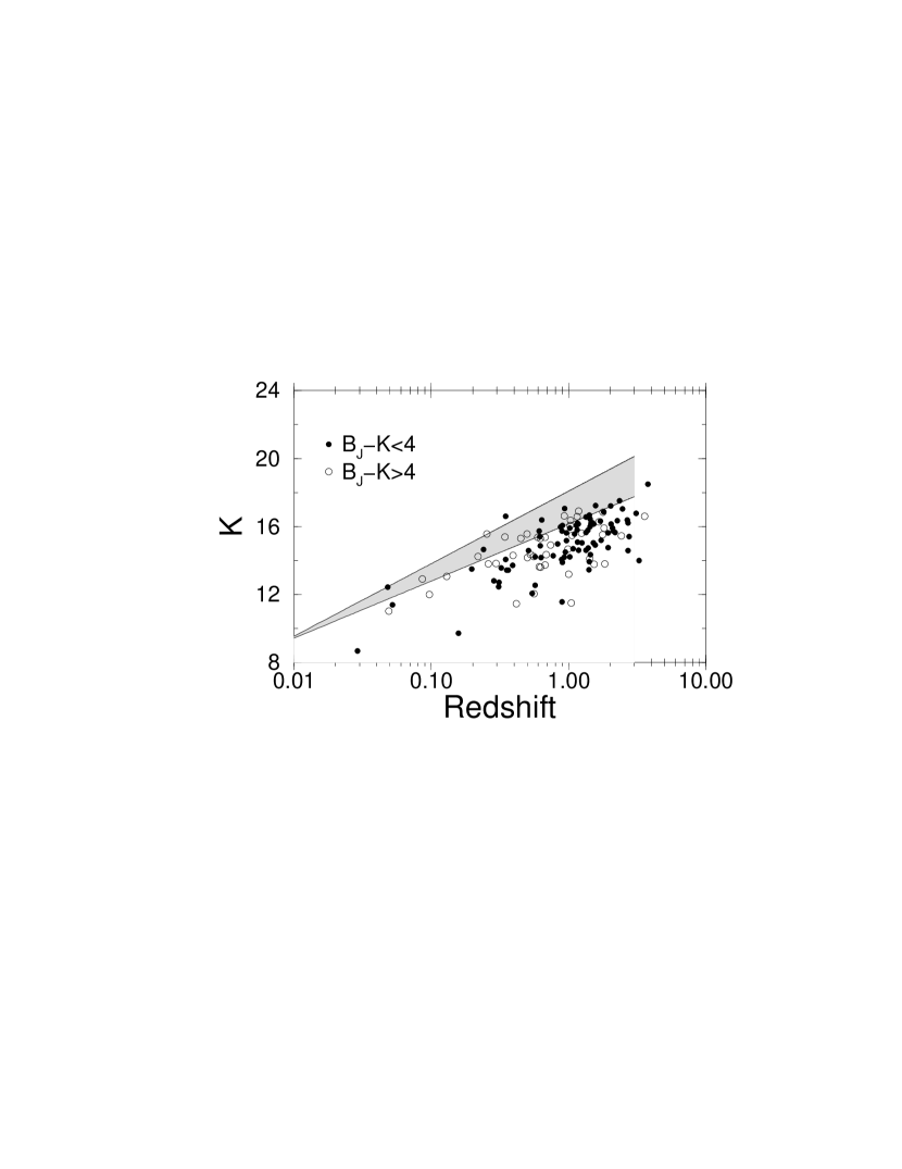
Figure 6.1: Observed $K$-$z$ relation for radio-loud ellipticals given by the shaded region which approximately corresponds to the spread in $K$ magnitudes (McCarthy, 1993). The open circles represent all Parkes sources with colours $B_{J}-K>4$ and filled circles are those with $B_{J}-K<4$.

Also plotted in Fig. 6.1 are the observed $K$ magnitudes for Parkes sources corresponding to colours $B_{J}-K<4$ (filled circles) and $B_{J}-K>4$ (open circles). Overall, very little overlap between the radio galaxy and Parkes magnitudes is observed. A majority of the Parkes sources are more than 2 magnitudes brighter than the mean in the galaxy $K$-$z$ relation. This cannot be explained by a possible difference in the size of aperture used in the photometry to determine $K$ magnitudes since it can only account for at most an uncertainty of $\sim 0.2$ mag in $K$ (McCarthy, 1993). Thus, if the host galaxies of Parkes sources have the typical $K$ magnitudes of radio galaxies, we estimate from Fig. 6.1 that the galaxy will only contribute on average $\raisebox{-3.01385pt}{\mbox{$\stackrel{{\scriptstyle\textstyle<}}{{\sim}}$}}20$% of the total light at $z\sim 1$.

There are also a number of sources in Fig. 6.1 which appear to lie within the shaded region of observed radio galaxy magnitudes. A majority of these do indeed show extended $K$-band images that can be interpreted as diffuse emission from a host galaxy. In fact, $\sim 10\%$ of Parkes sources have extended $K$-band images that can be attributed to a galaxy component.

We conclude that as a first measure, a majority of Parkes sources appear significantly brighter at near-IR wavelengths than the locus defined by radio galaxies in the $K$-$z$ relation. Emission from the central AGN is likely to dominate the near-IR flux and hence $B_{J}-K$ colours observed in Parkes sources. This conclusion is strongly supported by the observation that a majority of Parkes sources appear very compact and bright in $K$. This is expected, since for quasars in general which comprise the majority of identifications in the Parkes sample, their redshifts are high enough that contamination by a red stellar component would be minimal.

6.3 Outline of Method

The galaxy contribution can be estimated using an algorithm that determines the relative strength of the characteristic 4000Å  break in the optical spectra of Parkes sources in an unbiased way. No other feature in a generic quasar spectrum will mimic this feature. In this section, we describe this algorithm.

6.3.1 Assumptions

There are two important assumptions that will be required by our algorithm. First, we assume that the spectral shape defining an underlying quasar optical continuum is ‘smooth’ and contains no breaks. This is justified by our current knowledge of quasar optical spectra. Our choice for this shape is somewhat arbitrary, and will be further discussed in section 6.3.2.

Second, we need to assume the input galaxy spectrum which defines the shape of the 4000Å  break to be used in our analysis. We have formed a composite optical spectrum of 18 Parkes sources all of which appear ‘spatially extended’ in $B_{J}$. This composite is shown as the solid curve in Fig. 6.2 and clearly shows the characteristic 4000Å  break. Superimposed (dashed) is an elliptical galaxy SED predicted from the stellar population synthesis models of Bruzual & Charlot (1995; see Bruzual & Charlot, 1993). This model is for a galaxy of age 8Gyr, and assumes a 1Gyr burst described by a Salpeter initial mass function with no star formation thereafter. In fact, any ‘old aged’ model with long completed star formation will in general be similar. Models assuming ‘long lived’ constant star formation rates lead to considerably bluer optical-UV continua, characteristic of those observed in spirals. The composite and model in Fig. 6.2 are in excellent agreement, except for the emission lines arising from ISM gas in the composite. In our analysis, we shall assume that this model represents the underlying elliptical SED in each of our Parkes sources.

Figure 6.2: Composite optical spectrum of 18 Parkes sources which appear spatially extended in $B_{J}$ (solid curve), and a model spectrum for an ‘old’ elliptical SED from Bruzual & Charlot (1993).

Figure 6.3: Spectral evolution of the 1Gyr burst model of Bruzual & Charlot (1993). The age in Gyr and the approximate corresponding redshift for a formation epoch $z_{f}=5$ with ($q_{0},h_{50}$)=(0.5,1) is shown beside each spectrum.

For sources with redshifts $z\raisebox{-3.01385pt}{\mbox{$\stackrel{{\scriptstyle\textstyle>}}{{\sim}}$}}1$, the $4000$Å  break is redshifted out of the wavelength range available in the spectra of Parkes quasars (see section 6.4.1) and thus, cannot be used in our algorithm. We are therefore restricted to $z<1$. For simplicity, we assume that the general shape or our model elliptical SED is independent of redshift to $z\sim 1$. The colours of radio galaxies observed to $z\sim 3$ are consistent with formation redshifts $4\raisebox{-3.01385pt}{\mbox{$\stackrel{{\scriptstyle\textstyle<}}{{\sim}}$}}z_{f}\raisebox{-3.01385pt}{\mbox{$\stackrel{{\scriptstyle\textstyle<}}{{\sim}}$}}20$ (Spinrad & Djorgovski, 1987; Dunlop $et\,al.$ 1989). These formation redshifts are also suggested by models of galaxy formation in the CDM scenario (eg. White & Frenk, 1991). The spectral synthesis models predict that the general form of an elliptical SED shown in Fig. 6.2 can be immediately established following an almost instantaneous ($\sim 1$Gyr) burst of star formation. Adopting the 1Gyr burst model of Bruzual & Charlot (1993) (updated 1995 models), we show in Fig. 6.3 the spectral evolution as a function of age since the initial starburst. Also shown beside each age is the approximate redshift for a formation epoch of $z_{f}=5$. Initially, the 4000Å  break region is diluted by starburst activity. After a few gigayears, the stellar population evolves passively, maintaining an almost uniform SED shape (see Bruzual & Charlot, 1993). For formation epochs $z\raisebox{-3.01385pt}{\mbox{$\stackrel{{\scriptstyle\textstyle>}}{{\sim}}$}}5$, it is apparent that the generic elliptical SED shape of Fig. 6.2 is easily established by $z\sim 1$.

6.3.2 The Algorithm

In general, the total flux at a given wavelength observed in a Parkes source, $f_{T}(\lambda)$, can be modelled as the sum of light contributed by the central quasar or AGN, $f_{q}(\lambda)$, and any underlying host galaxy $f_{g}(\lambda)$ (eg. Fig. 6.2). We write the relationship between these quantities as:

$$f_{q}(\lambda)\,=\,f_{T}(\lambda)-c\,f_{g}(\lambda),$$ (6.1)

where $c$ is a scaling factor giving an arbitrary measure of the amount of galaxy light we wish to determine for a particular source.

Given $f_{T}(\lambda)$ for a particular source and an arbitrary galaxy spectrum $f_{g}(\lambda)$ (Fig. 6.2), our aim is to determine the value of $c$ such that $f_{q}(\lambda)$ looks something like a quasar spectrum. From our knowledge of quasar optical spectra, an obvious choice is to require that $f_{q}(\lambda)$ be “smooth” and contain no breaks. Thus, the basis of this algorithm involves subtracting an arbitrary amount of galaxy flux, $c\,f_{g}(\lambda)$ from $f_{T}(\lambda)$ such that the resulting spectrum $f_{q}(\lambda)$ appears smooth (see below). When this is achieved, the fraction of total light at a given wavelength contributed by the host galaxy can be estimated by normalising:

$$F_{gal}(\lambda)\,=\,\frac{c\,f_{g}(\lambda)}{f_{T}(\lambda)}.$$ (6.2)

In order to implement the above algorithm, we need to define an acceptable form for the shape of the quasar spectrum $f_{q}(\lambda)$. Our only requirement is that this spectrum be smooth and hence our choice is somewhat arbitrary. We choose $f_{q}(\lambda)$ to be a power-law, parameterised by:

$$f_{q}(\lambda)\,=\,f_{q}(\lambda_{max})\left(\frac{\lambda}{\lambda_{max}}\right)^{\alpha},$$ (6.3)

where the slope $\alpha$ is determined between two fixed wavelengths, $\lambda_{min}$ and $\lambda_{max}$ (see below):

$$\alpha\,=\,\frac{\ln\left[f_{q}(\lambda_{min})/f_{q}(\lambda_{max})\right]}{\ln\left[\lambda_{min}/\lambda_{max}\right]}.$$ (6.4)

Using Eqn. 6.1, the fluxes defined in Eqn. 6.4 can be written:

$$f_{q}(\lambda_{min})\,=\,f_{T}(\lambda_{min})-c\,f_{g}(\lambda_{min})$$ (6.5)

$$f_{q}(\lambda_{max})\,=\,f_{T}(\lambda_{max})-c\,f_{g}(\lambda_{max}).$$

For a discussion on how the wavelengths $\lambda_{min}$ and $\lambda_{max}$ are chosen and the fluxes in Eqn. 6.5 measured, see section 6.4.1.

To apply this algorithm in a self consistent way to each of our optical spectra, we need to define a figure of merit indicating the point at which the maximum amount of galaxy spectrum has been subtracted and a “smooth” quasar spectrum (ie. a power-law) is achieved. Let us first consider the rest frame optical spectrum of a source, $f_{T}(\lambda)$, suspected of containing a 4000Å  break. This is illustrated in Fig. 6.4. Furthermore, let us consider a “smooth” power-law (ie. the underlying quasar spectrum $f_{q}(\lambda)$) between two wavelengths $\lambda_{min}$ and $\lambda_{max}$ on either side of the 4000Å  break region as shown. We define our figure of merit as representing the area $A$ of the shaded region in Fig. 6.4. As certain amounts of galaxy spectrum, $c\,f_{g}(\lambda)$ (where $f_{g}(\lambda)$ is given by Fig. 6.2) are gradually subtracted from $f_{T}(\lambda)$, $A$ will decrease and becomes a minimum when the break disappears. We can thus determine the value of $c$ when this occurs, allowing us to estimate the fractional galaxy contribution from Eqn. 6.2.

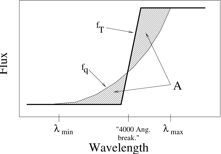
Figure 6.4: Definition of our “figure of merit” $A$. For a particular source spectrum $f_{T}(\lambda)$ (whose 4000Å  break region is shown exaggerated), we subtract an amount of galaxy flux, $f_{g}(\lambda)$ (Fig. 6.2) until $A$ is a minimum and a smooth power-law $f_{q}(\lambda)$ results.

For a given amount of subtracted galaxy flux, $c\,f_{g}(\lambda)$, we can write $A$ in terms of $c$ from Eqn. 6.1 as follows:

$$A\,=\,\int^{\lambda_{max}}_{\lambda_{min}}{\left|f_{q}(\lambda)-f_{T}(\lambda)+c\,f_{g}(\lambda)\right|}\,\,d\lambda.$$ (6.6)

With $f_{q}(\lambda)$ defined by Eqns. 6.3, 6.4 and  6.5, $A$ can be written:

$$A\,=\,\int^{\lambda_{max}}_{\lambda_{min}}\left|\left[f_{T}(\lambda_{max})-c\,f_{g}(\lambda_{max})\right]\left(\frac{\lambda}{\lambda_{max}}\right)^{\alpha(c,f_{T},f_{g})}-\,f_{T}(\lambda)+c\,f_{g}(\lambda)\right|\,\,d\lambda,$$ (6.7)

where $\alpha(c,f_{T},f_{g})$ is defined by Eqns. 6.4 and  6.5. Thus, one would only have to minimise $A$ with respect to $c$ in order to determine the maximal galactic contribution. We introduce however, an additional factor in Eqn. 6.7 whose purpose will be to make best use of the available data and optimise our algorithm.

Data Optimisation

Due to systematic effects, each Parkes optical spectrum suffers from a considerable amount of noise at the range of observed wavelengths. Although the noise may have some wavelength dependence, we assume it is constant. Given this assumption, we have used an optimal method that gives more weight to those wavelengths in a particular spectrum where the residual $\left|f_{q}(\lambda)-f_{T}(\lambda)\right|$ (see Fig. 6.4) is likely to be a maximum. In other words, the galaxy subtraction process will depend most sensitively on the spectral shape around the 4000Å  break region. Our assumption that the noise is wavelength independent will greatly simplify our optimisation method, since otherwise, we would have to simultaneously optimise those observed spectral regions with the highest signal-to-noise.

The basis of this method simply involves convolving the integrand in Eqn. 6.7 with a weighting function $G(\lambda)$ that gives more weight to regions on either side of the $4000$Å  break within $\lambda_{min}<\lambda<\lambda_{max}$ (see Fig. 6.4). We choose to define $G(\lambda)$ purely from the galaxy spectrum $f_{g}(\lambda)$ (dashed curve in Fig. 6.2). This is defined as the difference (or residual) between a power-law and the galaxy spectrum within the range $\lambda_{min}<\lambda<\lambda_{max}$, containing the $4000$Å  break:

$$G(\lambda)\,=\,\left|f_{gPL}(\lambda)-f_{g}(\lambda)\right|,$$ (6.8)

where

$$f_{gPL}(\lambda)\,=\,f_{g}(\lambda_{max})\left(\frac{\lambda}{\lambda_{max}}\right)^{\alpha_{g}}$$

and

$$\alpha_{g}\,=\,\frac{\ln\left[f_{g}(\lambda_{min})/f_{g}(\lambda_{max})\right]}{\ln\left[\lambda_{min}/\lambda_{max}\right]}.$$

The function $G(\lambda)$ will peak at wavelengths on either side of the $4000$Å  break. Thus, by convolving $G(\lambda)$ with Eqn. 6.7, relatively more weight will be given to spectral data at these wavelengths, where our algorithm is most sensitive.

Figure 6.5: Examples of our figure of merit function $A$ (defined by Eqn. 6.9) as a function of the parameter $c$. Source spectra are shown in Fig. 6.6.

Thus, the function to minimise can now be written:

$$A\, = \,\int^{\lambda_{max}}_{\lambda_{min}}\put(0.0,20.0){\line(0,-1){35.0}}\left[f_{T}(\lambda_{max})\,-\,c\,f_{g}(\lambda_{max})\right]\left(\frac{\lambda}{\lambda_{max}}\right)^{\alpha(c,f_{T},f_{g})}$$ (6.9)

$${\rm\hskip 36.135pt}\,-\,f_{T}(\lambda)\,+\,c\,f_{g}(\lambda){\rm\hskip 3.61371pt}\put(0.0,20.0){\line(0,-1){35.0}}\,\,\,G(\lambda)\,\,d\lambda,$$

where $G(\lambda)$ is defined by Eqn. 6.8. Our aim is to determine the value of $c$ for a particular source spectrum $f_{T}(\lambda)$ such that $A$ is a minimum. In Fig. 6.5, we show examples of the figure of merit function $A$ (Eqn. 6.9) as a function of the parameter $c$ for two sources whose spectra are shown in Fig. 6.6. If the weighting factor $G(\lambda)$ in Eqn. 6.9 is neglected, we find that the values of $c$ at which $A$ is a minimum decrease by up to $5\%$ in most sources where the break feature appears relatively weak or absent. In sources with strong 4000Å  breaks, there is no significant difference. Given the value of $c$ that minimises $A$, the fractional galaxy contribution at some wavelength can now be computed using Eqn. 6.2.

6.3.3 Error Determination

In spectra where the galaxy contribution is relatively weak, an upper limit on its contribution at some appropriate level of significance would be required. In order to do so, both random and systematic errors need to be investigated. The magnitude of these two types of errors are estimated and compared in section 6.5.2. Here, we briefly outline the method in their determination.

Random (Statistical) Errors

The random error at some confidence level in the galaxy contribution is estimated by computing the value of $c$ corresponding to the statistical error in $A$ (Eqn. 6.9). Since Eqn. 6.9 is actually a discrete sum over wavelength bins $\lambda_{i}$, from $\lambda_{min}$ to $\lambda_{max}$, the statistical error is determined by adding the error for each individual bin in quadrature, so that

$$\sigma(A)\,=\,\sqrt{\sum_{\lambda_{i}=\lambda_{min}}^{\lambda_{max}}\sigma^{2}_{i}(I)},$$ (6.10)

where $\sigma_{i}(I)$ is the error in the integrand $I$ of Eqn. 6.9 for bin $\lambda_{i}$. $\sigma_{i}(I)$ will depend only on uncertainties in the measured source fluxes $f_{T}(\lambda_{max})$ and $f_{T}(\lambda_{min})$ in Eqn. 6.9. As shall be discussed in section 6.4.1, these fluxes are estimated by calculating the median continuum flux in wavelength bins centered on $\lambda_{max}$ and $\lambda_{min}$. We estimate the corresponding uncertainties by computing the rms deviation from the mean spectral flux in these wavelength bins.

Systematic Errors

Our definition of the underlying quasar continuum $f_{q}(\lambda)$, in each source only requires that it be smooth and contain no breaks. This implies that the shape of $f_{q}(\lambda)$ is somewhat arbitrary and thus it is possible that our quantitative measures of the galaxy contribution may strongly depend on its assumption in our algorithm. The uncertainty introduced by this possible systematic effect will be investigated.

All our calculations assume that $f_{q}(\lambda)$ is a power-law (ie. Eqn. 6.3), since the continua of optical quasar spectra are well represented by $f_{\nu}\propto\nu^{-\alpha}$ where $\alpha\sim 0.2-0.3$ (Francis, 1996). To investigate the effects of assuming a different form for $f_{q}(\lambda)$ however, we also apply our algorithm by assuming for simplicity that $f_{q}(\lambda)$ is a straight line joining $\lambda_{min}$ and $\lambda_{max}$ in Fig. 6.4. This is parameterised as follows:

$$f_{q}(\lambda)_{line}\,=\,\frac{\left[f_{q}(\lambda_{max})-f_{q}(\lambda_{min})\right]}{\lambda_{max}-\lambda_{min}}(\lambda-\lambda_{max})\,+\,f_{q}(\lambda_{max}),$$ (6.11)

where $f_{q}(\lambda_{min})$ and $f_{q}(\lambda_{max})$ are defined by Eqn. 6.5. A comparison in the fractional galaxy contributions resulting from our use of a power-law (Eqn. 6.3) and a straight line (Eqn. 6.11) for $f_{q}(\lambda)$ in our algorithm, will enable us to estimate the magnitude of this systematic effect. Results are presented in section 6.5.2. Other possible sources of systematic error are also discussed in this section.

6.3.4 Summary

To summarise, we have presented in this section a method to determine the relative galaxy contribution in each Parkes source in a robust way. Our algorithm requires the following two input assumptions: First, an elliptical optical SED, $f_{g}(\lambda)$, defining the shape of the characteristic 4000Å  break. This we assume is a model from Bruzual & Charlot (1993) (see Fig. 6.2). Second, we require a spectral shape defining the underlying quasar spectrum $f_{q}(\lambda)$. Unless otherwise specified, all our calculations shall assume a power-law for $f_{q}(\lambda)$.

With the only requirement that $f_{q}(\lambda)$ be smooth and contain no breaks, the “suspected” 4000Å  break in each source spectrum $f_{T}(\lambda)$, is subtracted until the residual between $f_{q}(\lambda)$ and galaxy subtracted source spectrum is a minimum. The galaxy contribution is estimated from the amount of galaxy, $f_{g}(\lambda)$ subtracted. To apply this procedure in a self-consistent manner, we have defined a figure of merit given by Eqn. 6.9. This is minimised with respect to the parameter $c$ from which the fractional galaxy contribution can be easily computed using Eqn. 6.2.

6.4 Data and Input Parameters

Out of the 323 sources in the Drinkwater $et\,al.$ (1997) sample, we have optical spectra for 194 or 60% of the sample. Some of these are from the compilation of Wilkes $et\,al.$ (1983) and others are from recent observations on the AAT and ANU 2.3m (see Drinkwater $et\,al.$ 1997). For these latter observations (65 sources), the spectra cover the observed wavelength range: $3200{\rm\AA}\raisebox{-3.01385pt}{\mbox{$\stackrel{{\scriptstyle\textstyle<}}{{\sim}}$}}\lambda\raisebox{-3.01385pt}{\mbox{$\stackrel{{\scriptstyle\textstyle<}}{{\sim}}$}}10000{\rm\AA}$ with a resolution of $\sim 5$Å  in the blue and $\sim 20$Å  in the red ($\raisebox{-3.01385pt}{\mbox{$\stackrel{{\scriptstyle\textstyle>}}{{\sim}}$}}5200$Å). Other spectra have typically a mean resolution $\sim 10$Å  and cover the range: $3200{\rm\AA}\raisebox{-3.01385pt}{\mbox{$\stackrel{{\scriptstyle\textstyle<}}{{\sim}}$}}\lambda\raisebox{-3.01385pt}{\mbox{$\stackrel{{\scriptstyle\textstyle<}}{{\sim}}$}}8000{\rm\AA}$.

6.4.1 Applying the Algorithm

Before applying our algorithm, each Parkes optical spectrum is redshifted to its rest frame. We then define the fixed rest frame wavelengths $\lambda_{min}$ and $\lambda_{max}$ within which the suspected 4000Å  break and our figure of merit (Eqn. 6.9) is defined (see Fig. 6.4). To choose these wavelengths, we need to consider the following:

First, the highest redshift sources will have the rest wavelength $\lambda_{max}$ redshifted out of the observational wavelength range of the spectra. These sources will not be able to be used in our algorithm. We therefore need to choose $\lambda_{max}$ such that the number of sources in which our algorithm can be applied is not significantly reduced. Second, we need a wavelength range $\lambda_{min}<\lambda<\lambda_{max}$ that makes ‘optimal’ use of the shape of the 4000Å  break region defining our figure of merit $A$ (the residual area in Fig. 6.4). In other words, we need to ensure that this region is unambiguously defined and clearly represented in each source spectrum. As a compromise, we assume $\lambda_{min}=3500$Å  and $\lambda_{max}=5080$Å  in every source.

Relative measures of the fluxes: $f_{T}(\lambda_{min,max})$ and $f_{g}(\lambda_{min,max})$ in the source and galaxy rest frame spectra respectively (see Eqn. 6.9), are determined as follows. We first define wavelength bins of width $\sim 200$Å  and $\sim 400$Å  centered on $\lambda_{min}$ and $\lambda_{max}$ respectively, and then calculate the median continuum flux in each bin. The wavelength regions defining these bins however may contain absorption and emission lines. Such lines are likely to bias our estimates of the continuum level in these regions. From the bin widths defined above, the rest wavelength regions of interest are: $3400{\rm\AA}<\lambda<3600$Å  and $4880{\rm\AA}<\lambda<5280$Å . From the available source spectra, we find that no lines are likely to contaminate the short wavelength bin. For the long wavelength bin however, we find that the emission line doublet [OIII]$\lambda\lambda$4959,5007 and a weak absorption feature at $\sim 5170$Å  (possibly from MgI) are strong contaminants. To avoid significant contamination, our algorithm excludes regions of width 10Å  centered on these lines.

Given the definitions above, our rest wavelength range required by our algorithm will therefore be $3400{\rm\AA}\raisebox{-3.01385pt}{\mbox{$\stackrel{{\scriptstyle\textstyle<}}{{\sim}}$}}\lambda_{rest}\raisebox{-3.01385pt}{\mbox{$\stackrel{{\scriptstyle\textstyle<}}{{\sim}}$}}5280{\rm\AA}$. With a maximum observed wavelength of $\lambda_{max}({\rm obs})\simeq 10000$Å  in $\sim 30\%$ of the available spectra, we find that only sources with redshifts $z\raisebox{-3.01385pt}{\mbox{$\stackrel{{\scriptstyle\textstyle<}}{{\sim}}$}}0.9$ can be used in our algorithm. In total, we have about 53 spectra in which our algorithm can be applied.

6.5 Results

6.5.1 Spectral Fits

With the input parameters from the previous section, Eqn. 6.9 is minimised numerically with respect to the parameter $c$ for each spectrum. Having found the value $c_{min}$ that minimises Eqn. 6.9, we can reconstruct the initial source spectrum $f_{T}(\lambda)$ by superimposing the maximum amount of galaxy spectrum, $c_{min}f_{g}(\lambda)$ generated by the algorithm, and a power-law representing the underlying “smooth” quasar continuum $f_{q}(\lambda)$. From Eqns. 6.1 and 6.3, these reconstructed model spectra can be represented:

$$f_{T}(\lambda)_{model}\, = \,c_{min}f_{g}(\lambda)\,+\,f_{q}(\lambda)$$ (6.12)

$$\equiv c_{min}f_{g}(\lambda)\,+\,\left[f_{T}(\lambda_{max})-c_{min}\,f_{g}(\lambda_{max})\right]\left(\frac{\lambda}{\lambda_{max}}\right)^{\alpha(c_{min},f_{T},f_{g})}.$$

A visual comparison between these model and observed spectra in the range $\lambda_{min}<\lambda<\lambda_{max}$ will allow us to investigate the accuracy of our algorithm in reproducing the observed spectra around the 4000Å  break region. Reconstructed spectra $f_{T}(\lambda)_{model}$ are compared with the observed spectra, $f_{T}(\lambda)$, for a number of sources in Fig. 6.6. On each spectrum, we also show our power-law fit $f_{q}(\lambda)$. As expected, observed spectra showing strong 4000Å  breaks with SEDs similar to that given in Fig. 6.2 are reproduced very accurately about the break region.

Figure 6.6: Observed rest frame spectra (dotted) for a number of sources in the Parkes sample. Also shown are reconstructed model spectra (solid) as defined by Eqn. 6.12 and power-law fits representing the underlying quasar continuum (dashed).

In a majority of observed spectra where no significantly strong breaks are discernible to the human eye however, our algorithm nevertheless attempts to fit for a break. Unbiased estimates of the galaxy contribution using the relative sizes of these breaks, however weak, are presented in section 6.5.3.

Fig. 6.6 continued.

6.5.2 Systematic vs. Random Errors

As discussed in section 6.3.3, a possible source of systematic uncertainty is in our assumption of the shape of the underlying smooth quasar continuum $f_{q}(\lambda)$. To explore this, we compare the relative galaxy contribution obtained by assuming first, a power-law (PL) (Eqn. 6.3) for $f_{q}(\lambda)$ and second, a straight line (L) (Eqn. 6.11). Using our algorithm and these two definitions for $f_{q}(\lambda)$, we have computed the fractional galaxy contribution at 5000Å  (rest frame). Results are shown in Fig. 6.7.

Figure 6.7: Fractional galaxy contribution at 5000Å  (rest frame) assuming a straight line for $f_{q}(\lambda)$ (vertical axis) and a power-law (horizontal axis). The diagonal line is the line of equality. (see section 6.5.2).

At first glance, estimates for the galaxy fraction using the power-law and straight line for $f_{q}(\lambda)$ agree very well. There is relatively little scatter about the diagonal line defining the equality ${\rm frac}_{L}={\rm frac}_{PL}$, except for a distinct population with ${\rm frac}_{L}<{\rm frac}_{PL}$. No distinguishing feature in the optical spectra of this latter class is immediately apparent. It is likely that a power-law (rather than a straight line) within $\lambda_{min}<\lambda<\lambda_{max}$ for these sources provides a better representation of our figure of merit $A$ in Fig. 6.4. We quantify the systematic error from the rms scatter in the difference: $\delta={\rm frac}_{L}-{\rm frac}_{PL}$, which we denote by $\sigma(\delta)$. For this systematic effect, we therefore estimate a $1\sigma$ uncertainty in the galaxy fraction at 5000Å  of at most $\sigma_{frac.}\simeq 0.02$.

Another possible source of systematic error is in our selection of the wavelengths $\lambda_{max}$ and $\lambda_{min}$, within which the suspected 4000Å  break and our figure of merit (Eqn. 6.9) is defined (see Fig. 6.4). As discussed in section 6.4.1, the values $\lambda_{min}=3500$Å  and $\lambda_{max}=5080$Å  were chosen as a compromise between: first, to maximise the number of sources in which the 4000Å  break remains within the observed wavelength after redshifting, and second, to make optimal use of the break region. What are the effects on the galaxy fraction if a different wavelength range were assumed?

To explore this, we choose to vary $\lambda_{max}$ alone. Due to the relatively small wavelength range at $\lambda<4000$Å  available in the galaxy spectrum (Fig. 6.2), we are not as flexible in varying $\lambda_{min}$. We therefore keep $\lambda_{min}$ fixed at 3500Å. Assuming the same bin widths (200Å  and 400Å ) centered on $\lambda_{min}$ and $\lambda_{max}$, and the PL definition for $f_{q}(\lambda)$, we have computed galaxy fractions at 5000Å  with $\lambda_{max}=5500$Å , and $\lambda_{max}=6500$Å . Combined with our estimates using $\lambda_{max}=5080$Å , we find that changing $\lambda_{max}$ makes negligible difference in the galaxy fraction. The fractions differ by no more than 1%.

We now compare these systematic uncertainties with estimates of the random errors. Fig. 6.8 shows the distribution of random errors in the fractional galactic contribution at 5000Å  as determined from our algorithm (see section 6.3.3). The range in random errors is significantly broad, with a majority of values exceeding our maximum $1\sigma$ systematic uncertainty of 0.02 deduced from Fig. 6.7. In the remaining sections, we therefore quote all uncertainties in the relative galaxy contribution as purely statistical, based on random errors alone.

Figure 6.8: Distribution of $1\sigma$ random errors in the fractional galaxy contribution at 5000Å (rest frame) for Parkes sources. (see section 6.5.2).

6.5.3 Galactic Contribution to the Observed Optical-Near IR Continuum.

Using our algorithm, we have computed the fractional galaxy contribution in the individual bandpasses $B_{J}$ $(\lambda\simeq 4400{\rm\AA})$ and $K$ $(\lambda\simeq 2.2\mu{\rm m})$, expected in an observer’s frame for each source. We estimate these using Eqn. 6.2 where fluxes are approximated by computing the median spectral flux at the central wavelength of each bandpass. Since our observed spectra do not extend to near-IR wavelengths, we estimate the observed spectral flux in $K$ using our observed $B_{J}-K$ colours and extrapolate from the spectral flux corresponding to $B_{J}$. Unfortunately, not all of the 53 sources used in our algorithm have a measured $K$ magnitude and hence $B_{J}-K$ colour. Of these sources, about 34 have known $K$ magnitudes.

The distributions in galaxy fractions in $B_{J}$ and $K$ are shown in Figs. 6.9a and b respectively. Sources with mean galaxy fractions $\raisebox{-3.01385pt}{\mbox{$\stackrel{{\scriptstyle\textstyle<}}{{\sim}}$}}5\%$ are replaced by their $3\sigma$ upper limits (dashed histograms). The distributions in Figs. 6.9a and b appear very similar, except however for a greater number of sources with galaxy contributions $>70\%$ in the $K$-band. These are all low redshift sources with strong 4000Å  breaks in their spectra. Their light is expected to be dominated by evolved stellar populations, and hence strongest in $K$. We must also note that the $B_{J}$ magnitudes used to estimate the $K$ spectral fluxes via $B_{J}-K$ colours are only accurate to $\sim 1$ mag (Drinkwater $et\,al.$ 1997). This photometric uncertainty is likely to contribute significant scatter in our estimates of the $K$ galaxy fraction in Fig. 6.9b.

We have divided the $K$-band identifications into two populations: those which show extended (resolved) structure, and those which remain unresolved. The galaxy fraction in $K$ for these two populations is shown as a function of $z$ in Fig. 6.10. Open symbols represent resolved sources, and filled symbols, unresolved sources. As expected, those sources exhibiting resolved structure are also those which show large galaxy fractions and are at relatively low redshifts.

Figure 6.9: (a) Distribution in fractional galaxy contributions in $B_{J}$ and (b) $K$ for $z<1$. Dashed portions represent $3\sigma$ upper limits, (see section 6.5.3).

We now investigate whether emission from the host galaxies of Parkes quasars can significantly contribute to their observed $B_{J}-K$ colours. We do this by computing the $B_{J}-K$ colour of the hypothesised underlying “quasar”, $(B_{J}-K)_{q}$, we would expect if contribution from the host galaxy was absent in each source. If the observed colours were entirely due to galactic emission, then we expect the distribution in $(B_{J}-K)_{q}$ to show a relatively small scatter, i.e. similar to that observed for optically selected quasars where typically $(B_{J}-K)_{q}\simeq 2.5$.

Figure 6.10: Fractional galaxy contribution in $K$ as a function of redshift for resolved sources (extended on $K$ and $B_{J}$ images; open symbols) and unresolved sources (closed symbols). Triangles represent $3\sigma$ upper limits on the galaxy fraction.

The colour of an underlying quasar, $(B_{J}-K)_{q}$, can be written in terms of the observed colour $(B_{J}-K)_{obs}$ and the galaxy fractional contributions $F_{gal}(B_{J})$ and $F_{gal}(K)$ as follows:

$$(B_{J}-K)_{q}\,=\,(B_{J}-K)_{obs}\,+\,2.5\log{\left[\frac{1-F_{gal}(K)}{1-F_{gal}(B_{J})}\right]}.$$ (6.13)

$(B_{J}-K)_{q}$ is plotted against $(B_{J}-K)_{obs}$ in Fig. 6.11a. As can be seen, the scatter in galaxy subtracted colours, $(B_{J}-K)_{q}$, remains and is extremely similar to that of the observed colour distribution. We quantify the galaxy contribution to the observed $B_{J}-K$ colours (in magnitudes) in Fig. 6.11b. From Figs. 6.11a and b, we conclude that the observed spread in colours cannot be due to emission from the host galaxies of Parkes quasars. An independent mechanism must be involved.

Figure 6.11: (a) Observed $B_{J}-K$ colour vs. colour of the underlying quasar (i.e. resulting galaxy subtracted colour: $(B_{J}-K)_{q}$). Error bars correspond to $1\sigma$ significance. (b) Distribution in galaxy contribution to observed $B_{J}-K$ colours in magnitudes.

6.6 A Test for the Unified Model

Studies of the host galaxy properties of BL-Lacs and radio-quasars can be used as a test of the unified scheme for radio-loud AGN. Motivated by the canonical axisymmetric model for AGN, the basis of this scheme is that the appearance of an extragalactic radio source is primarily determined by viewing geometry. Extended FRI and FRII-type radio galaxies are believed to represent the parent (misaligned) populations of the more compact BL-Lacs and radio quasars respectively (Urry & Padovani, 1995 and references therein). If classification is purely based on orientation, then intrinsic properties such as host galaxy luminosity should be approximately uniform throughout. In this section, we shall test this hypothesis.

Studies have shown that for quasars and FRII radio galaxies at redshifts $z\raisebox{-3.01385pt}{\mbox{$\stackrel{{\scriptstyle\textstyle<}}{{\sim}}$}}0.3$, the situation is not entirely clear. From comparisons of their mean host galaxy luminosities, some studies have shown that FRII hosts are fainter by $\sim 0.5$-1 mag. (Smith & Heckman, 1989), while others have concluded that they are comparable (eg. Taylor $et\,al.$ 1996). The main difficulty in these studies was finding sufficiently large samples of radio galaxies and quasars matched both in radio power and redshift. There is strong observational evidence however that the low redshift BL-Lacs reside in giant ellipticals with mean optical luminosities and de Vaucoleurs $r^{1/4}$ law profiles similar to those in FRIs (Ulrich, 1989; Stichel $et\,al.$ 1993). Very little is known about the host galaxies of compact radio sources at higher redshifts. Using our algorithm however, we can get estimates of host galaxy $K$ magnitudes for sources up to $z\sim 1$.

We can predict the host galaxy $K$ magnitudes of Parkes sources directly from our estimates of the fractional galaxy contribution in the $K$-band, $F_{gal}(K)$ (see section 6.5.3). The host galaxy magnitude in an observer’s frame can be written:

$$K_{gal}\,=\,K_{source}\,-\,2.5\log{\left[F_{gal}(K)\right]},$$ (6.14)

where $K_{source}$ is the observed $K$ magnitude of the source. As discussed in section 6.5.3, $F_{gal}(K)$ is determined from the median spectral flux at $\lambda\simeq 2.2\mu$m (Eqn. 6.2), which we estimate using the observed spectral flux at $\lambda\simeq 4400$Å  and $B_{J}-K$ colour.

Estimates of $K_{gal}$ as a function of redshift are shown in Fig. 6.12. For comparison, we also show the range observed for radio galaxies (shaded region) as determined from a number of independent studies (McCarthy, 1993; see section 6.2). Within our quoted uncertainties, there appears to be no significant difference in the mean host galaxy magnitude of “compact” Parkes sources and extended radio galaxies at the redshifts indicated. The compact sources however appear to show a larger scatter in $K_{gal}$ at some redshift. Since the $K_{gal}$ values were determined from non-contemporaneous measures of observed $B_{J}$ spectral fluxes and $B_{J}-K$ colours, this may be attributed to variability in the underlying AGN. We are unable at present to quantify this uncertainty. From Fig. 6.12, we conclude that the host galaxy luminosities of these two classes of radio source is consistent with that required by the unified model.

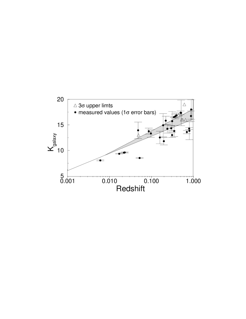
Figure 6.12: Host galaxy $K$ magnitude as a function of redshift for Parkes sources (symbols) and the range observed for radio galaxies (shaded region; McCarthy, 1993).

6.7 Discussion

Our results of section 6.5.3 clearly show that galactic emission is unlikely to fully explain the dispersion in $B_{J}-K$ colours observed. This conclusion is only valid however for sources at redshifts $z\raisebox{-3.01385pt}{\mbox{$\stackrel{{\scriptstyle\textstyle<}}{{\sim}}$}}0.9$. At higher redshifts, the 4000Å  break feature on which our algorithm is based is redshifted out of our observational wavelength range. Taking into account our completeness in spectral data (section 6.4), only 53 of the 323 sources in the Drinkwater $et\,al.$ (1996) sample have been analysed using our algorithm.

Since we are limited to redshifts $z\raisebox{-3.01385pt}{\mbox{$\stackrel{{\scriptstyle\textstyle<}}{{\sim}}$}}0.9$, it is possible that we are biased towards detecting relatively large galaxy contributions. Galaxy flux will be more easily detected at the lowest redshifts. This indeed may appear to be the case if we compare the fractional galaxy contribution in $K$ from our algorithm (Fig. 6.9b), with that predicted from the Hubble diagram (Fig. 6.1) containing sources to $z\sim 3$. Comparing the radio galaxy and source $K$ magnitudes, the Hubble diagram predicts a “mean” fractional galaxy contribution of $\sim 20\%$ for redshifts $z\raisebox{-3.01385pt}{\mbox{$\stackrel{{\scriptstyle\textstyle<}}{{\sim}}$}}3$, while the mean in Fig. 6.9b is $\sim 50\%$. This discrepancy is expected since galactic flux for sources at $z>0.9$ will obviously be relatively weak.

We have three pieces of observational evidence that supports a minimal galaxy contribution from the high redshift sources: First, all sources with $z\raisebox{-3.01385pt}{\mbox{$\stackrel{{\scriptstyle\textstyle>}}{{\sim}}$}}0.5$ appear very compact in $K$ (eg. Fig. 6.10), and exhibit broad-line equivalent widths typical of those observed in quasars in the optical. Second, the observed $B_{J}-K$ colours correlate with optical-UV continuum slope (see section 5.5.2), implying that optical-UV colours are also relatively red and display large scatter. The observed optical-UV colours of ellipticals at $z\raisebox{-3.01385pt}{\mbox{$\stackrel{{\scriptstyle\textstyle>}}{{\sim}}$}}0.9$ however are observed to be quite blue (Guiderdoni & Rocca-Volmerange, 1987 and references therein) and hence cannot explain this observation. Third, significantly high levels of linear polarisation ($\raisebox{-3.01385pt}{\mbox{$\stackrel{{\scriptstyle\textstyle>}}{{\sim}}$}}5\%$) are observed at near-IR wavelengths in a majority of sources (see Chapter 7). This strongly indicates that the emission is dominated by a non-thermal mechanism.

6.8 Conclusions

In this chapter, we have investigated whether emission from the host galaxies of Parkes quasars can significantly contribute to the relatively large spread in $B_{J}-K$ colours observed. If the hosts are classical giant ellipticals and their flux strongly contributes, then this would be expected since elliptical colours are known to be quite red in $B-K$ to $z\sim 2$.

We have devised an algorithm that measures the relative galaxy contribution in each source in an unbiased way using the characteristic 4000Å  break feature of elliptical galaxy SEDs. The basis of the algorithm involves subtracting a generic elliptical SED from each source spectrum until the 4000Å  break feature disappears and what is left is a “smooth” spectrum containing no breaks. This “smooth” spectrum we refer to as the underlying quasar continuum. The only requirement by our algorithm is that this remaining spectrum be smooth. The galactic contribution, relative to the total light at any wavelength is estimated from the amount of galaxy subtracted.

The main conclusions are:
1. For $z\raisebox{-3.01385pt}{\mbox{$\stackrel{{\scriptstyle\textstyle<}}{{\sim}}$}}0.9$, (for which the 4000Å  feature remains observable in our spectra), we find broad and almost bimodal distributions in the relative galaxy fraction in $B_{J}$ and $K$. Most sources ($\raisebox{-3.01385pt}{\mbox{$\stackrel{{\scriptstyle\textstyle>}}{{\sim}}$}}70\%$) have galaxy fractions $<0.3$ at the $3\sigma$ level in both $B_{J}$ and $K$. The remainder have large galaxy contributions and are predominately low redshift galaxies with strong 4000Å  breaks. All of these latter sources are spatially extended and resolved on $B_{J}$ and $K$-band images. In particular, there is a clear distinction in the strength of the 4000Å  break for resolved and unresolved sources.
2. Using these estimates, we find that the mean $K$-band magnitude of the host galaxies of flat spectrum radio quasars is consistent with that of extended radio galaxies at $z\raisebox{-3.01385pt}{\mbox{$\stackrel{{\scriptstyle\textstyle<}}{{\sim}}$}}0.9$. This is consistent with the unified model for radio-loud AGN.
3. By subtracting the galaxy contribution in each bandpass from the observed $B_{J}-K$ colours of Parkes sources, we find that at the $1\sigma$ confidence level, the relatively large spread in colours still remains. We conclude that in a majority of cases, the relatively red colours must be due to a mechanism other than that contributed by a “red” stellar component.

Chapter 7 A Search for Near-Infrared Polarisation

“For the truth of the conclusions of physical science, observation is the supreme Court of Appeal.”

— Sir Arthur Eddington,

The Philosophy of Physical Science, 1958

7.1 Introduction

As explored in previous chapters, the two primary models used to explain the redness observed in Parkes quasars are: the synchrotron emission model and the dust model. We can further distinguish between these two models using broadband polarimetry. In the near-infrared, both the strength and wavelength dependence of linear polarisation should be different for each of these mechanisms.

Linear polarisation is an excellent signature of synchrotron emission (Pacholczyk, 1970). If the reddening in Parkes quasars is due to a red synchrotron component dominating the near-IR flux, then strong polarisation is expected. Observations of the wavelength dependence of polarisation in a number of flat spectrum radio-quasars shows that the polarisation generally decreases strongly with decreasing wavelength from the near-IR to optical (eg. Wills $et\,al.$ 1988; 1992). This can be explained if the synchrotron continuum is diluted by unpolarised light from the “big blue bump” emission responsible for photoionizing emission line regions.

This wavelength dependence has mostly been observed in the optically brightest and “bluest” radio-quasars with $B\raisebox{-3.01385pt}{\mbox{$\stackrel{{\scriptstyle\textstyle<}}{{\sim}}$}}16$ mag. Observations by Wills $et\,al.$ (1992) and Impey & Tapia (1990) find that about half of their flat-spectrum radio sources are polarised in the optical with $3\%\raisebox{-3.01385pt}{\mbox{$\stackrel{{\scriptstyle\textstyle<}}{{\sim}}$}}p_{V}\raisebox{-3.01385pt}{\mbox{$\stackrel{{\scriptstyle\textstyle<}}{{\sim}}$}}20\%$. Due to the faintness of many of the “reddest” Parkes quasars in the optical however, little information on their optical polarisation properties exists. Most of these red sources however are relatively bright in the near-IR ($K_{n}\raisebox{-3.01385pt}{\mbox{$\stackrel{{\scriptstyle\textstyle<}}{{\sim}}$}}14$) where broadband polarimetry is possible.

As shown in Chapter 5, if the reddest Parkes quasars are to be explained purely by the synchrotron model, then the spectra require particle energy distributions that are nearly monoenergetic or step-like in nature. Such particle distributions make a number of other predictions for the wavelength dependence of polarisation that can also be tested.

For the dust reddening model, both the strength and wavelength dependence of linear polarisation is expected to be different from that in the synchrotron model. If the dust and physical conditions in reddened Parkes quasars is similar to that in the galactic ISM, then polarisations from magnetically aligned dust grains of order a few percent in $K$ are expected (eg. Whittet, 1992 and references therein). As observed in the Galaxy, the linear polarisation shows a wavelength dependence that increases with decreasing wavelength primarily in the near-IR. Thus, the wavelength dependence of polarisation in the synchrotron and dust model are expected to be different in the near-IR. By measuring the linear polarisation in the near-IR, we may be able to unequivocally distinguish between these two models.

The observations presented in this chapter are designed to search for linear polarisation in the near-infrared in a number of red quasars. Our aim is to determine whether there are any sources with dust-like wavelength dependences in polarisation as well as exploring the previous modelling of the polarisation dependence in (blue) radio-quasars.

This chapter is organised as follows: In sections 7.2 and 7.3, we describe our observations and data reduction. Results are presented in section 7.4 and compared with previous polarisation studies in the optical where available. Possible evidence for variability and implications for the reddening mechanism are also discussed. In section 7.5, we briefly outline the predictions of a number of polarisation mechanisms and compare them with the data. In section 7.6, we analyse our results using fits of a two-component model for the source emission. This model also includes the possible effects of reddening by dust. Implications and further predictions are discussed in section 7.7, and all results are summarised in section 7.8.

7.2 The Observations

Observations were made on the 4 nights of 27th Feb. - 2nd Mar. 1997 using the infrared imager and spectrometer (IRIS) mounted at the Cassegrain focus of the 3.9m Anglo Australian Telescope at Siding Spring. IRIS was used in its polarimetry mode with the $f/15$ intermediate field setup (the polarimeter was provided by Prof. J. Hough of the University of Hertfordshire). The detector is a hybrid array of $128\times 128$ pixel format made of mercury cadmium telluride. The image scale is $0.61^{\prime\prime}$ per pixel for the $f/15$ intermediate field setup and corresponds to a field of view of $\sim 1.2^{\prime}$. This setup was used to allow for good sampling in the moderate seeing conditions typical at Siding Spring. Before describing our broadband polarimetry measurements, we first give a brief review of the method used to measure linear polarisation with the IRIS polarimeter.

7.2.1 Measuring the Polarisation with IRIS

Our aim is to measure the degree of polarisation. This is achieved by measuring the Stokes parameters, three of which are relevant for linear polarisation. One of the parameters, $I$, is the total intensity of the light, both polarised and unpolarised. The other two, normally called $U$ and $Q$, characterise the degree of polarisation along two orientations, with the plane of polarisation separated by $45^{\circ}$ (see below). To measure either $U$ or $Q$ along a given angle on the sky, the intensity of the light is measured through a polariser aligned along some direction (giving intensity $I_{1}$) and the intensity measured with the polariser at right angles to this (giving $I_{2}$). One Stokes parameter is then given by (say $U$):

$$U\,=\,\frac{I_{1}-I_{2}}{I_{1}+I_{2}},$$ (7.1)

where we have normalised with respect to the total intensity: $I=I_{1}+I_{2}$. Likewise, the other Stokes parameter ($Q$) is defined analogously, but with the plane of polarisation rotated by $45^{\circ}$ relative to its initial orientation. Given orthogonal component intensities $I_{3}$ and $I_{4}$ in this new orientation, we have:

$$Q\,=\,\frac{I_{3}-I_{4}}{I_{3}+I_{4}}.$$ (7.2)

See Fig. 7.1 for a schematic representation.

Once the Stokes parameters are measured, the fractional polarisation $P$ and its orientation $\theta$ can be found. Let us assume that the incident light is the incoherent sum of an unpolarised beam of intensity $I_{u}$ (which contributes equally to each orthogonal component image; see Fig. 7.1), and a perfectly linearly polarised beam of intensity $I_{p}$ with the $E$ vector lying at an angle $\theta$ to the instrument’s reference angle. It can be shown by simple trigonometry from Fig. 7.1 that the Stokes parameters (Eqns. 7.1 and 7.2) can be written:

$$U\,=\,\frac{I_{p}\cos{2\theta}}{I_{p}+2I_{u}},$$ (7.3)

$$Q\,=\,\frac{I_{p}\sin{2\theta}}{I_{p}+2I_{u}}.$$

The fraction of the total light in the polarised component (the percentage polarisation) is then defined:

$$P(\%)\,=\,100\frac{I_{p}}{I_{p}+2I_{u}}\,\equiv\,100\sqrt{U^{2}+Q^{2}},$$ (7.4)

and its orientation is given by:

$$\theta\,=\,0.5\,{\rm Tan}^{-1}{\left(\frac{Q}{U}\right)}.$$ (7.5)

Figure 7.1: Schematic representation of the components of the polarisation vector with intensity $I_{p}$. The sets of orthogonal components (images) $I_{1},I_{2}$ and $I_{3},I_{4}$ are used to compute the two relevant Stokes parameters $Q$ and $U$. $I_{u}$ is the unpolarised beam which contributes equally in each component such that the total intensity is $I_{TOT}=I_{p}+I_{u}$.

IRIS measures the two orthogonal polarisations (ie. $I_{1}$ and $I_{2}$ or $I_{3}$ and $I_{4}$ above) simultaneously using a Wollaston prism made of ${\rm Mg}{\rm F}_{2}$ - a birefringent material. The structure of the material is such that the velocities of the light ray will depend upon the polarisation of the radiation, and hence, two components polarised in different directions will be refracted by different amounts when emerging from the prism. This produces two images on the same chip, one in the “ordinary” light (ie. that polarised in one direction, say $I_{1}$ above), and the other in the “extraordinary light” (that polarised in the orthogonal direction, ie. $I_{2}$). The light rays producing these two images are usually referred to as the ‘o-ray’ and ‘e-ray’.

In principal then, since the “orthogonal” intensities $I_{1},I_{2}$ (Eqn. 7.1) or $I_{3},I_{4}$ (Eqn. 7.2) can be measured simultaneously, a Stokes parameter ($U$ or $Q$) can be measured from a single exposure. In practice however, there will be some instrumental polarisation originating primarily from inclined planar reflections in the optical elements. To take this out, the observing sequence on the IRIS polarimeter consists by following each exposure with a second one with the plane of polarisation rotated by $90^{\circ}$. What was the “ordinary image” (say $I_{1}$) is now the “extraordinary” image ($I_{2}$), ie. the two will have flipped places on the chip. This will allow any instrumental polarisation to be calibrated out and shall be discussed in more detail in our reduction procedure in section 7.3.1.

The plane of polarisation is rotated by using an optical element known as a half-waveplate above the fixed Wollaston prism. This device is also made of birefringent material and is rotated until the o- and e-rays travel in the same direction. The emergent rays will have altered phase delay relative to each other and hence with the polarisation vector rotated. A general plan of the major optical components in the IRIS polarimeter is shown in Fig. 7.2.

Thus, a measure of the linear polarisation is obtained by taking 4 exposures, each of which contains two orthogonal polarisations (images) on the same chip. The first pair of exposures has the plane of polarisation separated by $90^{\circ}$ and are combined to measure one of the Stokes parameters (see section 7.3.1). The second pair also contains polarised images with the polarisation vector separated by $90^{\circ}$. This pair however has the plane of polarisation displaced by $45^{\circ}$ relative to the first pair and are combined to measure the other Stokes parameter. Once the Stokes parameters are known, the fractional polarisation and its orientation can be computed from Eqns. 7.4 and 7.5.

Figure 7.2: Basic setup of optical components in the IRIS polarimeter.

7.2.2 Observational Strategy

The seeing during our observing run ranged from $4^{\prime\prime}$ (FWHM) on the first night to $0.8^{\prime\prime}-1.5^{\prime\prime}$ for the subsequent 3 nights. Observing conditions were mainly photometric throughout. We obtained polarimetric images for 9 sources in total from our sample of flat spectrum radio sources (Drinkwater $et\,al.$ 1997). In order to reasonably model the wavelength dependence of polarisation, we obtained images in $J$, $H$ and $K_{n}$ for most of these sources. Follow-up observations showed that three of the sources are identified as moderately red quasars (with optical continuum slopes $\alpha_{opt}\raisebox{-3.01385pt}{\mbox{$\stackrel{{\scriptstyle\textstyle>}}{{\sim}}$}}1$ and colours $B_{J}-K_{n}\raisebox{-3.01385pt}{\mbox{$\stackrel{{\scriptstyle\textstyle>}}{{\sim}}$}}4$), three as ‘blue’ quasars, and three as BL-Lac objects. A further discussion on individual source characteristics is given in section 7.4. Contemporaneous measurements in the $J$, $H$ and $K_{n}$ bandpasses was required to obtain a reliable polarisation spectrum, as the polarisation in such sources may vary substantially with time (eg. Impey & Tapia, 1990).

If the reddening in Parkes quasars is due to dust, then using empirical relations between extinction and polarisation from dust in the galaxy (see section 7.5.1), we predict for a mean observed reddening of $A_{V}\sim 2$, a polarisation of order a few percent in $K_{n}$. Due to the possibility of such relatively low levels, we initially sought to measure a $1\%$ polarisation at $5\sigma$ confidence level. Since crudely, $\sigma_{p}\sim\sigma_{U}/I\,\sim\sigma_{Q}/I$ (where $I$ is the total intensity), we estimated that a $S/N\sim 500$ in each of the individual 4 exposures (required for a polarisation measure-see above) was required. However, the accuracy of our measurements is mainly limited by photon statistics because of the faintness of our sources in the near-infrared. For a quasar with $K_{n}\sim 15$ (or $H,J\sim 16$), this would have taken $\sim 3$ hours integration time. Since the observations are sky limited ($S/N\propto c\sqrt{t}$, where $c$ are the counts and $t$ the exposure time), if the magnitude were increased by one, the exposure time would be increased by a factor of 6.25. The reddest of our sources have typically $J-K_{n}\sim 2$ and hence a red source with $K_{n}\sim 15$ implies more than 12 hrs integration in $J$. Thus, to keep the integration times short and maximise the number of objects that can be measured, we only observed red sources with $K_{n}<14$.

Our aim of a Poisson uncertainty of 0.2% in a 1% polarisation level is unlikely to be limited by other sources of contaminant polarisation. An example may be polarisation from transmission through aligned dust grains in the galaxy. All sources however have galactic latitude $>20^{\circ}$ where measurements of the polarisation towards distant stars suggest $p_{V}\raisebox{-3.01385pt}{\mbox{$\stackrel{{\scriptstyle\textstyle<}}{{\sim}}$}}0.2\%$ (Markkanen, 1979) and hence $p_{K}\raisebox{-3.01385pt}{\mbox{$\stackrel{{\scriptstyle\textstyle<}}{{\sim}}$}}0.1\%$ using the empirical polarisation law. Furthermore, the IRIS polarimeter is capable of an accuracy $\sigma_{p}=\pm 0.01\%$, given at least $10^{8}$ photons. The analysing efficiency is close to 100% as demonstrated by inserting a wire-grid (polariser) calibrator into the beam and as confirmed using polarised standards.

As discussed above, 4 separate exposures corresponding to different rotations of the half-waveplate are required to measure the two relevant Stokes parameters and hence polarisation. The observing sequence for each source and each band $J$, $H$ and $K_{n}$, consisted of repeated sets of these 4 exposures with each set corresponding to a raster position on the sky. For each consecutive set of four exposures, the raster positions were displaced by $\sim 30^{\prime\prime}$ east to west on the CCD chip. Each individual exposure consisted of effectively 60 second integrations (formed from repeated integration cycles) at which sufficient photons were accumulated. The sets of rasters were formed close enough to each other in time as possible so that uncertainties caused by variations in sky brightness and its polarisation are minimised when the sets are combined to form ‘sky frames’. This ensured that the final signal-to-noise in the ‘sky-subtracted’ polarimetric images was maximised (see section 7.3 for more details).

On the 3 nights at which the seeing was reasonably good (ie. $\sim 1^{\prime\prime}$), typical “total” integration times for our brightest sources (with $K_{n}\simeq 11-12$ mag) were about 30 min in each band. For fainter sources with $K_{n}\raisebox{-3.01385pt}{\mbox{$\stackrel{{\scriptstyle\textstyle>}}{{\sim}}$}}13$, total integration times were of order 60-90 min. Approximately $\sim 120$ min was spent in $J$ for our faintest source with $K_{n}\sim 14.4$. A log of our observations is shown in Table 7.1. Total numbers of rasters and exposures (each of effectively 60 sec. duration for all bands) are shown. A more complete description of the identification of each source from its optical spectrum is given in Table 7.2. Column 4 in Table 7.1 lists the $K_{n}$ magnitudes as measured from previous runs by P. Francis and M. Drinkwater (private communication). The dates of observation for these magnitudes are given in parentheses.

Source	RA (B1950)	Dec (B1950)	$K_{n}$ (Date)	Exposure (min.)
				J	H	$K_{n}$
PKS0537$-$441	05 37 21.00	$-$44 06 46.8	11.56 (13 Feb 95)	$14\times 4$	$14\times 4$	$14\times 4$
PKS0622$-$441	06 22 02.68	$-$44 11 23.0	14.34 (12 Feb 95)	-	-	$10\times 4$
PKS0829+046	08 29 10.89	+04 39 50.8	11.37 (25 Apr 94)	$7\times 4$	$7\times 4$	$7\times 4$
PKS1020$-$103	10 20 04.18	$-$10 22 33.4	13.50 (13 Feb 95)	$14\times 4$	$14\times 4$	$14\times 4$
PKS1036$-$154	10 36 39.48	$-$15 25 28.1	14.37 (3 Apr 94)	$21\times 4$	$30\times 4$	$21\times 4$
PKS1101$-$325	11 01 08.51	$-$32 35 06.2	13.43 (12 Feb 95)	$14\times 4$	-	$14\times 4$
PKS1313$-$333	13 13 20.05	$-$33 23 09.7	12.28 (25 Apr 94)	$7\times 4$	$7\times 4$	$7\times 4$
PKS1510$-$089	15 10 08.90	$-$08 54 47.6	13.44 (13 Aug 95)	$14\times 4$	-	$14\times 4$
PKS1546+027	15 46 58.29	+02 46 06.1	11.45 (12 Aug 95)	$14\times 4$	$14\times 4$	$14\times 4$

Table 7.1: Summary of observations.

7.3 Data Reduction

The initial stages of the CCD reductions were carried out using the FIGARO package which includes software specifically designed for the IRIS detector. This comprised mainly of corrections for bias and dark current and non-linearity between photon counts and output electrons. The final stages were carried out using the IRAF package. The principal tasks here were flat-field corrections, bad pixel corrections, sky subtractions and integrated photometry. Each of these steps is discussed in turn below.

BIAS AND DARK CURRENT: We first subtracted the readout ‘bias level’ and ‘dark current’ from each frame. The bias level is the offset value which a CCD adds to a signal before it converts its output to digital values. It allows the zero light level to be kept at a positive value, and avoids feeding negative values to the A/D converter. For the IRIS detector, the bias counts (typically 25,000-30,000 counts/pixel) are sufficiently uniform from pixel to pixel that they can be corrected for by subtracting the ‘dark current’ alone. The dark current of a CCD, which includes the bias level, is due to an accumulation of thermally created photons within the silicon multiplex layer that register as counts. This also includes stray photons that may be present in the IRIS dewar. Dark frames were taken with exposure times identical to those of the individual data frames with the shutter closed. The dark current was estimated to be relatively low, which averaged $\raisebox{-3.01385pt}{\mbox{$\stackrel{{\scriptstyle\textstyle<}}{{\sim}}$}}0.1$cnts/pixel/sec. The noise associated with readout of the CCD was also considerably low, being $<3$cnts rms over the entire chip.

NON-LINEARITY: The conversion of the numbers of photons falling onto the CCD chip into output electron counts is not perfectly linear. This particularly applies when the number of incident photons is relatively high or nears saturation (typically 65,000 cnts/pixel for the IRIS chip). Corrections for non-linearity in the IRIS chip involves computing correction factors from polynomial fits to the ‘count vs. photon’ relation for each pixel. This is built into the FIGARO software.

FLAT FIELDS: The sensitivity of a CCD chip is generally not uniform. Differences from pixel-to-pixel most commonly arise from imperfections introduced during the manufacturing process. These include variations in pixel sizes and quantum efficiency changes across the chip. To correct for these effects, we divided each data exposure by a similar exposure taken through the same filter. The flat field image must be taken on a uniformly emitting source. Our flat fields were obtained by exposing the chip on a uniformly illuminated section of the inside of the dome. These ‘dome flats’ were formed by subtracting flat-fields with the dome lamp off from those with the lamp on. The reason for this was so to correct for any thermal glow associated with the telescope, the instrument, and the inside of the dome. In addition to the pixel sensitivity variations, the IRIS chip has a considerable number of intrinsically “bad” pixels which were also corrected for by interpolating over them. Once the above corrections were applied, the frames were flat to better than 1% of sky.

SKY SUBTRACTION: In order to correct for uncertainties caused by temporal variations in sky brightness, polarisation and instrumental ‘glow’, and hence increase the final signal-to-noise ratio in images, a sky frame needs to be formed and subtracted from the data frames. As discussed above, raster positions were formed for every consecutive set of 4 exposures ($\sim 4$ min), each of which corresponds to a different waveplate position as required for a polarisation measure. To minimise variations in sky brightness, sky frames were formed by taking a median of 5 to 7 data frames corresponding to the same waveplate position from the rasters. These sets of sky frames were then subtracted from the initial data frames (taken at approximately the same time as the respective sky frames) corresponding to the respective waveplate positions. This yielded a signal-to-noise ratio $\sim 5$ times greater than before sky subtraction.

PHOTOMETRY: Once data frames were sky subtracted, integrated counts for each of the two images on each frame (ie. corresponding to the orthogonal ‘e’ and ‘o’ polarisation states - see section 7.2.1) were estimated using normal aperture photometry. For the fainter sources, the seeing conditions presented the major limitation, and for these, the accuracy of the counts was improved by using larger apertures on the sky. For each source then, we have 4 frames each containing 2 images. These can now be used to calculate the polarisation and its position angle as discussed in the following section.

7.3.1 Instrumental Effects and Measuring the Polarisation

As discussed in section 7.2.1, the Stokes parameters $U$ and $Q$ (Eqns. 7.1 and 7.2) contain all the information needed to compute the fractional linear polarisation. To compute each Stokes parameter, we have two frames, each taken with the plane of polarisation rotated by $90^{\circ}$. As discussed, these two frames are to be used to correct for any possible instrumental polarisation. For one of the Stokes parameters (say $U$), let us call these the $A$ and $B$ frames. Each frame contains two images, the ‘ordinary’ ($O$) and the ‘extraordinary’ ($E$) image. The same applies for the second pair of frames used to compute the $Q$ Stokes parameter, whose plane of polarisation is rotated through $45^{\circ}$ relative to the first pair. To compute each Stokes parameter then, we have 4 fluxes, let us call these: $AO$, $AE$, $BO$, and $BE$. Figure  7.3 shows a schematic representation.

Figure 7.3: Vectorial representation of the $4\times 2$ images which correspond to components of the polarisation vector P.

There are two algorithms that we can use for measuring the Stokes parameters from these 4 fluxes (J. Bailey; private communication), a ‘subtraction’ algorithm and a ‘ratio’ algorithm. The former is likely to give a slightly better signal-to-noise ratio if conditions are fairly uniform (as it uses arithmetic rather than geometric means for the latter).

For the first algorithm, the first step is to construct a correction factor $R_{inst}$ for any instrumental polarisation. This would show up as a systematic difference between the $O$ and $E$ images. If there was no such effect, $AE$ and $BO$ should be identical, and $BE$ and $AO$ likewise. This correction factor is given by:

$$R_{inst}\,=\,\frac{AE+BE}{AO+BO}.$$ (7.6)

There is a second correction factor we can form to account for possible variations in transparency between the $A$ and $B$ frames. If sky transparency fluctuations are negligible, the sum $AO+AE$ and $BO+BE$ should be identical. The relevant correction factor can thus be written:

$$R_{see}\,=\,\frac{AO+AE}{BO+BE}.$$ (7.7)

The Stokes parameter (say $U$; Eqn. 7.1) can be computed by averaging over the $A$ and $B$ frames ($I_{1}=(AO+BE)/2$ and $I_{2}=(AE+BO)/2$), and modifying these by the above correction factors so that:

$$U\,=\,\frac{R_{inst}AO+R_{see}BE-(AE+R_{inst}R_{see}BO)}{R_{inst}AO+R_{see}BE+AE+R_{inst}R_{see}BO}.$$ (7.8)

The same applies for the second set of frames (Fig. 7.3b) to estimate $Q$. If $R_{inst}$ and $R_{see}$ are stable during the night (or over a given set of data frames), they can be measured to high precision, increasing the final signal-to-noise.

The second algorithm uses a ratio technique. Firstly, a ratio is calculated:

$$r\,=\,\left(\frac{AO}{AE}\frac{BE}{BO}\right)^{1/2},$$ (7.9)

which is the geometric mean of the ratio of image intensities along two orthogonal polarisations. Any one of the Stokes parameters (say $U$) is then given by:

$$U\,=\,\frac{r-1}{r+1}.$$ (7.10)

This ratio technique normalises out instrumental polarisation effects as well as atmospheric transparency variations, though it is likely to give a lower final signal-to-noise ratio.

We have computed the correction factors $R_{inst}$ and $R_{see}$ (Eqns. 7.6 and 7.7) for each set of 4 frames in each night and found that they were reasonably constant, varying by $\raisebox{-3.01385pt}{\mbox{$\stackrel{{\scriptstyle\textstyle<}}{{\sim}}$}}3\%$ around unity for the brighter sources ($K_{n}\simeq 11$) and $\raisebox{-3.01385pt}{\mbox{$\stackrel{{\scriptstyle\textstyle<}}{{\sim}}$}}7\%$ for the fainter sources ($K_{n}\raisebox{-3.01385pt}{\mbox{$\stackrel{{\scriptstyle\textstyle>}}{{\sim}}$}}13$). Thus we have used the first algorithm above to compute our Stokes parameters. For the repeated sets of 4 frames we have for each source (in $J$, $H$ and $K_{n}$; see Table 7.1), average values of the correction factors and hence Stokes parameters (Eqn. 7.8) were computed. Statistical errors in Stokes parameters were computed by finding the rms uncertainty over a given set of frames, $\sigma_{rms}$, so that final Poisson uncertainties in the mean values can be estimated: $\sigma_{p}\simeq\sigma_{rms}/\sqrt{N}$, where $N$ is the number of (sets of 4 waveplate) observations. Thus, by taking repeated sets of observations (ie. increasing $N$), it can be seen that the final signal-to-noise ratio can be significantly improved.

For comparison, we also computed the Stokes parameters and errors using the ‘ratio technique’ and found that signal-to-noise ratios were lower by up to 5% than those found with the ‘subtraction’ algorithm. Once the Stokes parameters and corresponding errors were known, the fractional polarisation and its orientation angle was computed from Eqns. 7.4 and 7.5. This orientation angle was converted into a position angle $\theta_{pa}$ on the sky by using a wire-grid calibrator (or polariser) in the beam path to calibrate the zero point and confirmed using polarised standards.

During the run, unpolarised standards were also taken so that integrated photometric magnitudes in $J$, $H$ and $K_{n}$ can also be determined. This was done by summing the counts in the two ‘orthogonal’ polarisation images on each frame and taking the mean over all frames. All results are presented in the next section.

7.4 Results

A summary of the source properties is given in Table  7.2. Sources have been divided into into 2 classes, classified according to their optical spectral properties. Optical spectra where available are shown in Fig. 7.4 and references are given in Table 7.2. Two of the BL-Lacs (PKS0537$-$441 & PKS0829+046) were initially selected on the basis of the absence of emission lines and relatively high levels of polarisation in the optical as found by previous authors. The quasars were all selected on the basis of strong to intermediate broad lines. The sources PKS1313$-$333 and PKS1546+047 were identified as quasars in the early 1970’s (Burbidge & Strittmatter, 1972) who claimed to detect lines of intermediate strength. Neither however have published spectra. To be certain of their classification, allowing for any possible variability over this period, optical spectra were obtained on the ANU 2.3m by P. Francis in April 1997. These observations revealed that the source PKS1313$-$333 now exhibits BL-Lac characteristics, and hence, is listed under the BL-Lac category in Table 7.2.

A description of the columns in Table 7.2 is as follows: Columns (1) to (4) list the source name, redshift, $B_{J}-K_{n}$ colour (from contemporaneous photometry; see below) and optical continuum slope, $\alpha_{opt}$, respectively (where $f_{\nu}\propto\nu^{-\alpha_{opt}}$). Column (5) gives a brief description of the relative strength of optical emission lines for each source (see Fig. 7.4 for optical spectra) and the relative amount of reddening as indicated by the optical slope alone. Balmer decrements (H$\alpha$/H$\beta$) where measurable are also shown. Spectrum references are given in parentheses.

Our selection of objects for this observing run was based on $B_{J}-K_{n}$ colours derived from $B_{J}$ and $K_{n}$ measurements taken at different epochs. Contemporaneous photometry was obtained by P. Francis in April 1997 on the ANU 2.3m. Significant differences in broadband magnitudes were obtained, resulting in revised colours for these sources. From the new spectroscopic and photometric observations, only three of the quasars (PKS0622$-$441, PKS1020$-$103 and PKS1036$-$154) appear ‘moderately reddened’ according to optical continuum slope and $B_{J}-K_{n}$ colour. None of these sources exhibit large Balmer decrements indicative of significant reddening by dust. The Balmer decrements for two of these red quasars however appear somewhat larger than those in the three ‘bluer’ quasars, suggesting extinction may be important.

Table 7.3 shows our measured $J$, $H$ and $K_{n}$ magnitudes from this polarisation run. For comparison, contemporaneous $J$, $H$ and $K_{n}$ measurements from a later observing run in April 1997 are also shown. RMS uncertainties based on noise statistics in these magnitudes are typically $\raisebox{-3.01385pt}{\mbox{$\stackrel{{\scriptstyle\textstyle<}}{{\sim}}$}}\pm 0.1$mag. Combining the two sets of $K_{n}$-band measures in Table 7.3 with those found from previous runs (ie. those listed in Table 7.1), we list in column (4) the maximum difference in $K_{n}$ magnitude ($K_{max}-K_{min}$) from measurements over these three epochs. See section 7.4.1 for more details.

A summary of our measurements of the percentage linear polarisation and position angle for $J$, $H$ and $K_{n}$ is given in Table 7.4. Column (2) lists the polarisations and associated rms uncertainties based on Poisson noise statistics. Column (3) lists the corresponding position angle in degrees with associated rms uncertainties. In column (4), we list for comparison optical polarisation measures (at an effective wavelength $\lambda=0.55\mu$m) where available from the studies of Impey & Tapia (1990) and Wills $et\,al.$ (1992). In Fig. 7.4 we show the dependence of our polarisation measures with wavelength including cases where an optical measure was available. On the right of each plot we show the optical spectra together with near-IR fluxes scaled from the $B$-band spectral flux using contemporaneous $B$, $J$, $H$ and $K$ magnitudes. The polarisation position angles ($\theta_{pa}$) do not show any significant wavelength dependence from $J$ to $K_{n}$ for each source. In most cases, a scatter of $\sim 20\%$ about the mean value in $\theta_{pa}$ for the three bands is observed.

Quasars
Source	$z$	$B_{J}-K_{n}$	$\alpha_{opt}$	Comments
(1)	(2)	(3)	(4)	(5)
PKS0622$-$441	0.688	4.25	1.24	‘moderately red’ with intermediate lines (W83)
PKS1020$-$103	0.196	3.92	1.01	‘moderately red’ with strong lines, H$\alpha$/H$\beta$=4.4 (D97)
PKS1036-154	0.525	4.91	2.27	‘red’ with strong lines, H$\alpha$/H$\beta$=4.6 (D97)
PKS1101$-$325	0.355	2.38	0.01	‘blue’ with strong lines, H$\alpha$/H$\beta$=3.9 (W83)
PKS1510$-$089	0.362	3.98	$-0.08$	‘blue’ with strong lines, H$\alpha$/H$\beta$=2.5 (W83)
PKS1546+027	0.415	4.42	0.13	‘blue’ with strong lines, H$\alpha$/H$\beta$=2.1 (S97)

BL-Lacs
Source	$z$	$B_{J}-K_{n}$	$\alpha_{opt}$	Comments
PKS0537$-$441	0.893	4.92	2.68	very weak lines (W86)
PKS0829+046	-	4.48	1.33	no lines visible (D97)
PKS1313$-$333	0.901	4.44	0.40	one weak line present (S97)

Table 7.2: Source properties; REFERENCES.—W83: Wilkes $et\,al.$ (1983); W86: Wilkes (1986); D97: Drinkwater $et\,al.$ (1997); S97: spectra provided by a run on the ANU 2.3m by P. Francis (April 1997).

Quasars
Source	27 Feb.-2 Mar. 1997			12-18 Apr. 1997			$\Delta K_{n}(max)$
(1)	(2)			(3)			(4)
	J	H	$K_{n}$	J	H	$K_{n}$
PKS0622$-$441	-	-	14.15	-	-	-	0.2
PKS1020$-$103	14.96	14.27	13.33	14.85	14.11	13.27	0.23
PKS1036$-$154	17.37	16.44	15.79	17.23	16.32	15.63	1.42
PKS1101$-$325	14.34	-	13.11	14.55	13.93	13.16	0.32
PKS1510$-$089	14.55	-	12.87	15.24	14.09	13.27	0.57
PKS1546+027	14.73	13.61	12.82	14.97	13.88	13.02	1.57

BL-Lacs
Source	27 Feb.-2 Mar. 1997			12-18 Apr. 1997			$\Delta K_{n}(max)$
	J	H	$K_{n}$	J	H	$K_{n}$
PKS0537$-$441	15.68	14.85	14.03	14.76	13.85	13.02	2.47
PKS0829+046	13.41	12.61	11.84	13.45	12.52	11.80	0.47
PKS1313$-$333	14.62	13.78	12.95	15.46	14.36	13.69	1.41

Table 7.3: Contemporaneous photometry. Combined with $K_{n}$ magnitudes from earlier runs (Table 7.1), column (4) lists the maximum difference in $K_{n}$ magnitude from these three epochs.

Quasars
Source	$p\pm\sigma(p)$ (%)			$\theta_{pa}$ (deg)			$p_{V}$ (%)
(1)	(2)			(3)			(4)
	J	H	$K_{n}$	J	H	$K_{n}$
PKS0622$-$441	-	-	$1.4\pm 0.9$	-	-	$3.2^{+1.0}_{-0.9}$	-
PKS1020$-$103	$1.7\pm 0.2$	$2.5\pm 0.4$	$1.8\pm 0.6$	$42.5^{+7.3}_{-8.3}$	$35.0^{+6.2}_{-6.9}$	$51.8^{+7.1}_{-8.1}$	0.58 (W92)
PKS1036$-$154	$2.8\pm 1.3$	$3.1\pm 1.5$	$5.4\pm 2.0$	$56.5^{+6.1}_{-5.2}$	$70.6^{+8.8}_{-9.1}$	$60.9^{+7.9}_{-8.2}$	-
PKS1101$-$325	$0.2\pm 0.3$	-	$0.3\pm 0.3$	$87^{+14.5}_{-11.1}$	-	$89^{+10.1}_{-9.5}$	-
PKS1510$-$089	$3.6\pm 0.2$	-	$2.7\pm 0.2$	$58^{+6.0}_{-5.2}$	-	$61^{+8.1}_{-7.2}$	$1.9\pm 0.4$ (I90)
PKS1546+027	$6.2\pm 0.2$	$8.5\pm 0.2$	$8.6\pm 0.2$	$5.0^{+1.1}_{-0.8}$	$3.7^{+0.9}_{-0.9}$	$3.7^{+0.7}_{-0.6}$	3.4 (W92)

BL-Lacs
Source	$p\pm\sigma(p)$ (%)			$\theta_{pa}\pm\sigma(\theta_{pa})$ (deg)			$p_{V}$ (%)
	J	H	$K_{n}$	J	H	$K_{n}$
PKS0537$-$441	$8.0\pm 0.5$	$8.7\pm 0.4$	$10.8\pm 0.8$	$31.8^{+5.5}_{-5.1}$	$34.4^{+6.3}_{-5.1}$	$28.8^{+4.1}_{-5.2}$	$10.4\pm 0.5$ (I90)
PKS0829+046	$12.0\pm 0.4$	$12.5\pm 0.2$	$13.6\pm 0.1$	$67\pm^{+7.1}_{-6.2}$	$69.0^{+7.1}_{-7.2}$	$69.0^{+6.9}_{-7.2}$	11.2 (W92)
PKS1313$-$333	$12.7\pm 0.3$	$12.9\pm 0.5$	$13.2\pm 0.5$	$3.5^{+0.6}_{-0.5}$	$2.0^{+0.3}_{-0.3}$	$2.6^{+0.4}_{-0.4}$	-

Table 7.4: Polarimetry results; REFERENCES.—I90: Impey & Tapia (1990); W92: Wills $et\,al.$ (1992).

Figure 7.4: Wavelength dependence of percentage polarisation (left) and total flux spectra (right). Polarisations in $J$, $H$ and $K$ are from this study. The total flux spectra include extrapolated fluxes from $J$, $H$ and $K$ photometric measurements.

Fig. 7.4 continued.

7.4.1 Polarisation versus Variability and $B-K$ Colour?

A comparison of the maximum difference in $K_{n}$ magnitudes measured from the three epochs (see column (4) in Table 7.3) with $K_{n}$ polarimetry measures for our six quasars shows a correlation between the two. This is shown in Fig. 7.5 (filled circles) and is significant at the $99\%$ confidence level. The three BL-Lacs however (open circles) are all highly polarised with $p_{K}>10\%$ and two show changes of $>1$ mag in $K_{n}$-band flux over a timescale of $\sim 2$ years.

The significant changes in $K_{n}$ flux for the highly polarised sources suggests variability in the source emission. If so, then a correlation with the degree of polarisation can be explained if the near-IR is dominated by “beamed” synchrotron emission, possibly from a relativistic jet. This mechanism both enhances the amplitude and decreases the timescale of flux variations in an observer’s frame. This is the standard model used to interpret the properties of highly variable AGN at optical and radio wavelengths, ie. the classical blazars and BL-Lac-type objects (eg. Königl, 1981), and is indeed consistent with observations of our three BL-Lacs in the near-infrared. Fig. 7.5 indicates that there are also sources with normal quasar-like properties in the optical but BL-Lac-like properties in the near-infrared. Relatively high near-IR polarisation levels in quasars which are ‘normal’ in the optical were also observed by Brindle $et\,al.$ (1986), Smith $et\,al.$ (1986) and Wills $et\,al.$ (1988).

The polarisations (and hence changes in $K_{n}$ flux) appear to have a bimodal distribution with respect to $B_{J}-K$ colour. The four bluest quasars (with $B_{J}-K_{n}$$\stackrel{{\scriptstyle\textstyle<}}{{\sim}}$4.4) in our sample are also those which exhibit the lowest polarisations as compared to the redder quasars and BL-Lacs with $p_{K}\raisebox{-3.01385pt}{\mbox{$\stackrel{{\scriptstyle\textstyle>}}{{\sim}}$}}5\%$. The $K_{n}$ polarisations are shown as a function of $B_{J}-K_{n}$ colour in Fig. 7.6. The relatively high near-IR polarisations (and variability) in the red quasars suggests that their colours may be associated with an intrinsically red synchrotron component dominating the near-IR flux. Implications of this result on models for the source emission and other reddening mechanisms will be discussed in section 7.7 .

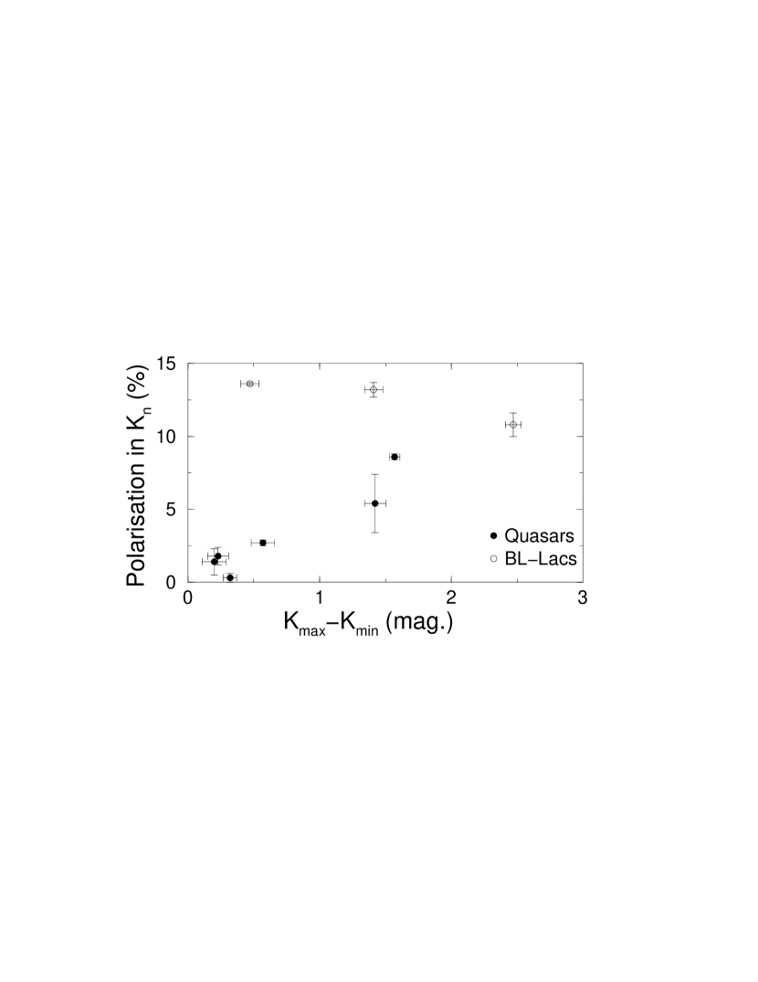
Figure 7.5: Polarisation at $K_{n}$ ($\lambda\simeq 2.1\mu$m) as a function of the difference in maximum and minimum $K_{n}$ magnitudes from measurements over three epochs (see section 7.4.1).

Figure 7.6: $K_{n}$-band polarisation as a function of $B_{J}-K_{n}$ colour.

7.5 Origin of the Polarisation?

The reddening models explored in the previous chapters make a number of specific predictions for both the strength and wavelength dependence of polarisation. In this section, we outline these predictions and compare them with the data. We shall primarily discuss three possible mechanisms that can give rise to a wavelength dependent polarisation. The first is polarisation by transmission through aligned dust grains. The second and third mechanisms are implied by the synchrotron reddening model. These are respectively: polarisation from a ‘pure’ synchrotron radiation spectrum and, a synchrotron spectrum modified by ‘unpolarised’ components which we refer to as the ‘two component model’. These are discussed in turn below.

7.5.1 Polarisation from Dust

If dust is contributing to the reddening observed in Parkes quasars, then we need to assume a model for the grains and physical conditions in order to explore the polarisation properties expected from the dust. As a first working hypothesis, we assume that the extinction and polarisation properties of the grains are the same as those derived from observations in the galaxy.

Transmission of light through aligned dust grains in the interstellar medium is responsible for the linear polarisation of starlight in our galaxy and other galaxies (Elvius 1978; Hough $et\,al.$ 1987; Clayton, Martin & Thompson, 1983). The accepted model is ‘linear dichroism’ or directional extinction resulting from the presence of non-spherical grains aligned by the galactic magnetic field. In the galaxy, the degree of polarisation in the visual passband ($\lambda\simeq 5500$Å) shows a correlation with the amount of reddening lying in the range:

$$P_{V}\,\simeq\,(2.3-9)E_{B-V}\,\,\%\,{\rm mag}^{-1},$$ (7.11)

or in terms of extinction:

$$P_{V}\,\simeq\,(0.6-2.2)A_{V}\,\,\%\,{\rm mag}^{-1}$$ (7.12)

(Serkowski $et\,al.$ 1975). The most efficient polarising medium is one where the grains can be modelled as ‘infinite cylinders’ (ie. length$\gg$radius) with diameters comparable to the wavelength, and their long axes parallel to each other. From Mie theory computations, such a model predicts a theoretical upper limit on the polarisation of

$$P_{V}\,\raisebox{-3.01385pt}{\mbox{$\stackrel{{\scriptstyle\textstyle<}}{{\sim}}$}}\,13.8A_{V}\,\,\%\,{\rm mag}^{-1}$$ (7.13)

(Whittet $et\,al.$ 1992 and references therein).

The wavelength dependence of linear polarisation from stars in the galaxy from the $K$ to $U$ passband has been described by the following empirical formula (Wilking $et\,al.$ 1982; Whittet $et\,al.$ 1992):

$$p(\lambda)\,=\,p_{max}\exp{\left[-C\ln^{2}{\left(\frac{\lambda_{max}(1+z)}{\lambda}\right)}\right]},$$ (7.14)

where $p_{max}$ is the maximum polarisation occurring at $\lambda_{max}$ and $C$ an inverse measure of the width of the polarisation curve. Observations show that $C$ and $\lambda_{max}$ are linearly related:

$$C\,=\,-0.1+1.86\lambda_{max}.$$ (7.15)

As discussed below, $\lambda_{max}$ is related to the average size of the polarising grains and lies in the range:

$$0.4\mu{\rm m}\raisebox{-3.01385pt}{\mbox{$\stackrel{{\scriptstyle\textstyle<}}{{\sim}}$}}\lambda_{max}\raisebox{-3.01385pt}{\mbox{$\stackrel{{\scriptstyle\textstyle<}}{{\sim}}$}}0.8\mu{\rm m},$$ (7.16)

with a mean value $0.55\mu$m for observations in the diffuse ISM. We have included the redshift factor $(1+z)$ in Eqn. 7.14 to account for the decrease in rest frame wavelength with source redshift. With $\lambda_{max}=0.55\mu$m, and adopting the upper bound $p_{max}=9E_{B-V}\%$ with a mean reddening $E_{B-V}\simeq 0.5$ ($A_{V}\simeq 2$), as inferred from the reddest Parkes quasars, Fig. 7.7 shows Eqn. 7.14 for three redshifts.

Figure 7.7: Wavelength dependence of polarisation as observed in diffuse regions of the galaxy for three redshifts of the dust. The polarisation levels are for optimum grain alignment, deduced from the polarisation-reddening relation (Eqn. 7.12) with $A_{V}=2$ - a mean value inferred from the reddest Parkes quasars.

The polarisation is seen to increase monotonically from $K$ to $V$-band wavelengths at the lowest redshifts, and this dependence remains strongest in the near-IR for dusty sources up to moderate redshifts; $z\raisebox{-3.01385pt}{\mbox{$\stackrel{{\scriptstyle\textstyle<}}{{\sim}}$}}1$. Within our interested wavelength range, ie. $J$ to $K$, the polarisation is predicted to decrease by as much as a factor of 3. The fact that this characteristic decrease in $p$ with $\lambda$ only occurs at the longest wavelengths ($\lambda>0.55\mu$m), is the crucial distinguishing feature of this model.

Comparison with Observations

As discussed above (see Table 7.2), we have three quasars in our sample whose optical continuum slopes appear moderately redder (with $\alpha_{opt}\raisebox{-3.01385pt}{\mbox{$\stackrel{{\scriptstyle\textstyle>}}{{\sim}}$}}1$) than those of the three bluer quasars having $\alpha_{opt}\raisebox{-3.01385pt}{\mbox{$\stackrel{{\scriptstyle\textstyle<}}{{\sim}}$}}0.1$. Although the Balmer decrements available for two of the ‘red’ quasars do not indicate significant amounts of dust along the line-of-sight, they are nonetheless consistent with their optical depths (see below) deduced from the slopes if we assume the intrinsic lower limit $H\alpha/H\beta\simeq 4$ (as observed in the ‘bluest’ radio-quasars where $H\alpha/H\beta=4.8\pm 0.9$; see section 5.5.3). These Balmer decrements are also on average larger than those of the bluer quasars in Table 7.2.

If the ‘moderate’ optical reddening in these sources were due to dust similar to that in diffuse regions of the galaxy, then what polarisation levels should we expect in the near-infrared? Assuming an ‘unreddened’ optical continuum slope of $\alpha_{opt}\simeq 0.3$ ($f_{\nu}\propto\nu^{-\alpha}$), which is a mean value observed for optically selected quasars (Francis, 1996), we can find approximate values for the extinctions, $A_{V}$ for our three quasars classified as moderately reddened in Table 7.2. From the optical continuum slopes, we find that in the rest frame, $A_{V}\simeq 0.6,\,0.7$ and 1.4 mag respectively for the sources: PKS0622$-$441, PKS1020$-$103 and PKS1036$-$154. Using the upper bound in the interstellar polarisation-reddening relation (Eqn. 7.12) to represent $p_{max}$ in Eqn. 7.14, we predict from Eqn. 7.14 with $\lambda_{max}=0.55\mu$m and $z=0.5$ that

$$P_{K}\,\raisebox{-3.01385pt}{\mbox{$\stackrel{{\scriptstyle\textstyle<}}{{\sim}}$}}\,0.8A_{V}\,\,\%\,{\rm mag}^{-1}.$$ (7.17)

For these sources specifically, upper limits in the $K$-polarisations predicted for the above extinction measures in an observer’s frame are respectively: $P_{K}\raisebox{-3.01385pt}{\mbox{$\stackrel{{\scriptstyle\textstyle<}}{{\sim}}$}}$0.7%, 0.5%, and 1.3%. As compared to the values observed: $P_{K}=1.4\pm 0.9\%$, $1.8\pm 0.6\%$ and $5.4\pm 2.0\%$, in only one case does the observed polarisation marginally agree within observational errors with the maximum value predicted for galactic-dust. The reddening observed in the other two sources is incompatible with their observed polarisation levels if due to dust like that in the local diffuse ISM.

Considerably greater grain alignment would be required for the observed polarisations in these sources to be due to transmission through aligned dust grains. The polarisation levels in $K$ are however consistent with the theoretical upper limit (Eqn. 7.13) for perfectly aligned grains modelled as ‘ideal’ infinite cylinders. If such grains are assumed to have diameter: $a\sim\lambda_{max}=0.55\mu$m and dielectric properties like those of in the galactic ISM, then the predicted wavelength dependence of polarisation (Greenberg, 1968) can be approximated using the galactic law (Eqn. 7.14). Using Eqn. 7.14 we find that this model predicts:

$$P_{K}\,\raisebox{-3.01385pt}{\mbox{$\stackrel{{\scriptstyle\textstyle<}}{{\sim}}$}}\,5A_{V}\,\,\%\,{\rm mag}^{-1}.$$ (7.18)

Table 7.5 summarises the predictions from Eqns. 7.17 and 7.18 for these three quasars. As one may expect, if the dust were located near the quasar central engine, the magnetic fields are likely to be strong, giving optimum grain alignment and hence high polarisation levels. The assumption of grain shapes in the form of ‘infinite cylinders’ on which Eqn. 7.18 is based however is an oversimplification and implausible. It is unlikely that transmission through aligned dust grains can fully explain the observed polarisation levels.

Source	$A_{V}$ (mag)	$P_{K}$(obs) (%)	$P_{K}$(gal)	$P_{K}$(theory)
PKS0622$-$441	0.6	$1.4\pm 0.9$	$<0.7$	$<3$
PKS1020$-$103	0.7	$1.8\pm 0.6$	$<0.5$	$<3.5$
PKS1036$-$154	1.4	$5.4\pm 2.0$	$<1.3$	$<7$

Table 7.5: Comparisons of $K$-polarisations in three ‘moderately reddened’ quasars, $P_{K}$(obs), with two dust model predictions: maximum value from measurements of local-galactic dust, $P_{K}$(gal) (Eqn. 7.17), and theoretical upper limit for perfectly aligned ‘ideal’ infinite cylinders, $P_{K}$(theory) (Eqn. 7.18).

It is immediately evident that in two of our moderately reddened quasars (PKS1020$-$103 and PKS1036$-$154) for which a polarisation spectrum could be deduced (Fig. 7.4), the wavelength dependence of polarisation cannot be fitted by the galactic-dust polarisation curve (Fig. 7.7) in the near-infrared. If an underlying dust-like polarisation spectrum were present and superimposed on a polarisation spectrum from an independent mechanism (say synchrotron-see next section), then the red quasars in our sample should systematically show a flatter polarisation curve on average than the bluer quasars. A comparison of the average polarisation slopes ($dP/d\lambda$) in these two ‘red’ quasars with the three ‘blue’ quasars however, shows that there is no significant difference.

If line-of-sight dust is contributing to the optical reddening observed in our three ‘moderately reddened’ quasars, then the polarisation data does not imply a total failure for this model. The polarisation observed from transmission through aligned dust grains in the galaxy is known to critically depend on a number of factors. The observed polarisation crucially depends on the orientation of the aligned grains and hence magnetic field relative to the observer. Since on average the magnetic field in the galaxy is parallel to the galactic plane (Heiles, 1987), grains will be aligned predominately in the plane of the line-of-sight, giving us an almost perfect geometry with which to observe interstellar polarisation through the galactic plane. Furthermore, theoretical models show that the grain alignment sensitively depends on the size, temperature and composition of the grains (Mathis $et\,al.$ 1986), as well as physical conditions of the associated gas component and nature of the radiation field (Whittet, 1992 and references therein). The presence of random or turbulent small scale magnetic fields along the line-of-sight can also significantly destroy uniformity in grain alignment on large scales. There is no doubt that the physical conditions in powerful radio-quasars are considerably different from those in the galaxy, and hence the presence of dust may not necessarily give a polarisation spectrum similar to that observed in the galactic ISM.

Mie theory computations show that the wavelength $\lambda_{max}$, corresponding to the maximum polarisation $p_{max}$ in Eqn. 7.14 is related to the average size of the polarising grains (Greenberg, 1968). Dielectric cylinders of radius $a$ and refractive index $n$ are shown to polarise most efficiently when $2\pi a(n-1)/\lambda\sim 1$ and thus, $\lambda_{max}\sim 2\pi a(n-1)$. Thus, the value $\lambda_{max}\simeq 0.55\mu$m as observed in the diffuse galactic ISM requires that $\langle a\rangle\simeq 0.15\mu$m for n=1.6 (typical of silicates). This is consistent with that predicted from the grain size distribution used to model the extinction curve. If the observed decrease in polarisation towards short wavelengths in our two red quasars were due to dust, then $\lambda_{max}$ would have to be at wavelengths $>2\mu$m in the rest frame. This is so that the region with $dP/d\lambda>0$ in the dust polarisation curve (Fig. 7.7) falls in the $J$, $H$ and $K$ passbands. A wavelength of $\lambda_{max}>2\mu$m would correspond to effective grain sizes $\sim 3.5$ times larger than those in the diffuse galactic ISM (for the same composition and geometry). Grain sizes this large however will cause very little optical-UV continuum reddening, contrary to that observed. Using the empirical relation, $R_{V}=A_{V}/E(B-V)\simeq 5.6\lambda_{max}$ for diffuse dust in the galaxy (Whittet & van Breda, 1978), we find that $\lambda_{max}>2\mu$m requires $R_{V}>10$ or $A_{B}/A_{V}<1.1$. The optical continuum reddening in Parkes quasars implies $A_{B}/A_{V}\raisebox{-3.01385pt}{\mbox{$\stackrel{{\scriptstyle\textstyle>}}{{\sim}}$}}1.3$, consistent with a $1/\lambda$ or galactic-type extinction law. Thus, such large grains cannot be responsible for both the reddening and polarisation observed.

On the basis of this very small sample of ‘reddened’ quasars, we conclude that absorption by aligned grains cannot explain their observed polarisation. If the observed reddening is to be attributed to dust, then the grains and/or physical conditions must be quite different from those found in the interstellar medium of our and other nearby galaxies. An alternative polarisation mechanism is required.

7.5.2 Polarisation from the Synchrotron Mechanism

‘Pure’ Synchrotron Emission

Polarisation is a well known property of the synchrotron process, being primarily due to the presence of ordered magnetic fields. Polarised emission is a characteristic exhibited by blazars and most flat radio spectrum core dominated sources, in most cases extending over more than five decades in frequency. Large polarisations ($>10\%$) in the optical continua of a significant number of core-dominant radio quasars are known to exist (eg. Impey & Tapia, 1990 and references therein), and provide strong evidence for a synchrotron component.

The percentage polarisation observed is dependent on a number of factors: firstly, on the magnetic field geometry, where it is greatest in the case when magnetic fields are highly aligned, secondly, on the spectral index of the emission spectrum and thirdly on the effects of depolarisation due to the presence of ionized plasma in front of the synchrotron source (eg. Faraday rotation). The effects of depolarisation by Faraday rotation are greatest at long wavelengths (mm to radio) where synchrotron self-absorption effects are important, while they are minimal at high frequencies (ie. optical to near-IR; Björnsson & Blumenthal, 1982).

Bjornsson & Blumenthal (1982) have shown that the fractional polarisation at some frequency $\nu$ expected from a synchrotron emitting plasma can be written

$$P(\nu)\,=\,{\cal F}(\nu)\left[\frac{1+\alpha(\nu)}{\frac{5}{3}+\alpha(\nu)}\right].$$ (7.19)

${\cal F}(\nu)$ is a factor describing the magnetic field geometry. For perfectly aligned fields, ${\cal F}(\nu)=1$, while as magnetic fields become more disordered, ${\cal F}(\nu)\rightarrow 0$. $\alpha(\nu)$ is the spectral index of the observed emission at the frequency $\nu$, where $f_{\nu}\propto\nu^{-\alpha(\nu)}$ and hence

$$\alpha(\nu)\,\equiv\,-\frac{d\ln f_{\nu}}{d\ln\,\nu}.$$ (7.20)

Thus, if the spectral index is independent of frequency as is the case if the particle energy distribution is a power law, and if ${\cal F}(\nu)$ is also constant, then the polarisation is frequency independent. The polarisation will be frequency dependent only for a synchrotron radiation spectrum which exhibits some degree of curvature (ie. where $\frac{d\alpha(\nu)}{d\ln{\nu}}\neq 0$).

Figure 7.8: Fractional polarisation as a function of the scaled frequency $\nu/\nu_{c}$ (where $\nu_{c}$ is defined by Eqn. 5.6) for a synchrotron spectrum exhibiting the maximum possible spectral curvature (eg. a monoenergetic synchrotron spectrum; see section 5.3.3). Typically, $\nu_{c}\sim 10^{13}$Hz and for this value, the $K$, $H$, $J$ and $B$ bands are also shown.

As discussed in section 5.3.3 of Chapter 5, a majority of the reddest Parkes sources (with say $B_{J}-K\raisebox{-3.01385pt}{\mbox{$\stackrel{{\scriptstyle\textstyle>}}{{\sim}}$}}5$) show concave-‘downward’ emission spectra (where $\frac{d\alpha(\nu)}{d\ln{\nu}}>0$) that are as extreme as can possibly be as predicted by conventional synchrotron models. Some of the sources require particle energy distributions that have to be nearly monoenergetic or “step-like” in nature. As discussed, the observed spectral curvature for such distributions will be the maximum possible via the synchrotron mechanism (ie. the single particle radiation spectrum, Eqn. 5.3). Thus, as predicted from Eqn. 7.19, this spectrum will lead to the strongest possible polarisation dependence with frequency. Combining Eqns. 5.3, 7.19 (with ${\cal F}(\nu)=1$) and 7.20, Fig. 7.8 shows this dependence in terms of the scaled frequency $\nu/\nu_{c}$, where $\nu_{c}$ is given by Eqn. 5.6. Typically, $\nu_{c}\sim 10^{13}$Hz - ie. the turnover frequency $\nu_{T}$ discussed in section 5.3.3.

As shown in Fig. 7.8, if the reddest Parkes quasars are due to a pure synchrotron radiation spectrum from a monoenergetic or step-like particle distribution, the polarisation is expected to increase with frequency. The frequency dependence will be strongest at the lowest frequencies. This characteristic dependence (with $dP/d\lambda<0$) has been observed in the optical-to-near-IR of a number of BL-Lac type objects by Brindle $et\,al.$ (1986). Polarisations as high as those shown in Fig. 7.8 have never been observed, and thus imply that either unpolarised components must be present (see next section) or that the emission may arise from regions without perfectly aligned magnetic fields.

The observed wavelength dependence of polarisation in our moderately reddened quasars (Fig. 7.4) is opposite to that predicted from a ‘pure’ synchrotron radiation spectrum exhibiting the maximum (‘concave downward’) spectral curvature (Fig. 7.8). To achieve polarisation spectra in this model that are compatible with the observations would require concave-‘upward’ total flux spectra (ie. $\frac{d\alpha(\nu)}{d\ln{\nu}}<0$; see Eqn. 7.8). This however would be contrary to the observed high frequency spectral shapes of our sources and blazar-like AGN in general (eg. see Fig. 5.5). We conclude that this mechanism alone cannot be used to explain the the polarisation and hence reddening observed. In the next section, we discuss a general model that may be more realistic of the emission mechanism in radio-quasars.

A Simple model with Two Spectral Components

Smith $et\,al.$ (1986) and Wills $et\,al.$ (1992) showed that the observed decrease in polarisation from near-IR to optical wavelengths in most core dominated radio quasars can be modelled using the sum of two spectral components. These components are as follows:

The first component is the ‘big blue bump’ (BBB) feature characteristic of the optical-UV continuum spectra of quasars. This is a broad feature with $\alpha\sim 0$ ($f_{\nu}\propto\nu^{-\alpha}$) lying between $\sim 1\mu$m and 1000Å  and is usually attributed to thermal emission from an accretion disk or optically thin free-free emission from hot gas (Barvainis, 1993 and references therein). This component is only weakly polarised, $P_{V}<1\%$, and is responsible for photoionizing emission line regions. The second component is a power-law ‘BL-Lac’ type component with $\alpha\sim 1-2$ which extends from the near-IR to optical-UV and is attributed to synchrotron emission. This component is assumed to have to have the same origin as that associated with the highly polarised and variable continua of BL-Lac objects. In most observations of BL-Lacs, the fractional polarisation of this almost pure synchrotron component is approximately independent of wavelength (eg. see sources in Fig. 7.4). If the synchrotron emission is relatively bright (eg. relativistically beamed), then contributions from unpolarised components in the near-IR such as emission from the host galaxy, emission lines and dust emission will be unimportant. By summing the unpolarised flat BBB component at short wavelengths with this polarised power-law synchrotron component, a decrease in polarisation towards shorter wavelengths is expected as the polarised power-law becomes increasingly diluted by the BBB.

If we denote the flux in the synchrotron component at some wavelength as $F_{s}(\lambda)$ with intrinsic wavelength independent polarisation $p_{s}$, and that in the BBB component as $F_{B}(\lambda)$, then the fractional polarisation can be written:

$$p(\lambda)\,=\,\frac{p_{s}F_{S}(\lambda)}{F_{S}(\lambda)+F_{B}(\lambda)}.$$ (7.21)

If we represent $F_{S}(\lambda)$ and $F_{B}(\lambda)$ in the rest frame as power-laws:

$$F_{S}(\lambda)\,=\,F_{S}(\lambda_{o})\left(\frac{\lambda}{\lambda_{o}}\right)^{\alpha_{{}_{S}}-2}\,\,{\rm and{\hskip 8.53581pt}}\,\,F_{B}(\lambda)\,=\,F_{B}(\lambda_{o})\left(\frac{\lambda}{\lambda_{o}}\right)^{\alpha_{{}_{B}}-2},$$ (7.22)

where $\alpha_{{}_{S}}$ and $\alpha_{{}_{B}}$ are power-law slopes ($f_{\nu}\propto\nu^{-\alpha}$), then the observed polarisation wavelength dependence can be written:

$$p(\lambda)\,=\,\frac{p_{s}}{1+f_{BS}(\lambda_{o})\left(\frac{\lambda}{\lambda_{o}}\right)^{\alpha_{{}_{B}}-\alpha_{{}_{S}}}(1+z)^{\alpha_{{}_{S}}-\alpha_{{}_{B}}}}.$$ (7.23)

The redshift factor accounts for the $K$-correction and $f_{BS}(\lambda_{o})$ represents the relative amount of BBB flux to synchrotron flux at $\lambda_{o}$, ie, $f_{BS}(\lambda_{o})\equiv F_{B}(\lambda_{o})/F_{S}(\lambda_{o})$.

An increase in the degree of relativistic beaming of the synchrotron component will cause the $p(\lambda)$ curve to approach the intrinsic polarisation $p_{s}$ of the synchrotron spectrum $F_{S}(\lambda)$. Any beaming factors will be contained in the normalisation factor $f_{BS}(\lambda_{o})$ in Eqn. 7.23. If $\delta$ is the Doppler factor, then $f_{BS}\propto\delta^{-(2+\alpha_{{}_{S}})}$ for a continuous jet and hence, $p(\lambda)\rightarrow p_{s}$ as $\delta\rightarrow\infty$. The total flux spectrum, $F_{TOT}(\lambda)=F_{S}(\lambda)+F_{B}(\lambda)$, will obviously steepen towards $F_{S}(\lambda)$ with slope $\alpha_{{}_{S}}$.

As a simple illustration, we assume the synchrotron ‘BL-Lac’ component has an intrinsic wavelength independent polarisation, $p_{s}=6\%$, and the ‘flat’ BBB component has $\alpha_{B}=0$. We assume these two components contribute equal flux densities at a rest wavelength $\lambda_{o}=7000$Å , ie. $f_{BS}(7000{\rm\AA})=1$. We take $z=0.5$. Fig. 7.9 shows $p(\lambda)$ for three values of the synchrotron power-law slope: $\alpha_{B}=0.5$, 1, 2. For comparison, the wavelength dependence of polarisation observed in two of our quasars from Fig. 7.4 having measured optical ($V$-band) polarisations from previous studies are also shown. PKS1546+027 is classified as a ‘blue’ quasar with $\alpha_{opt}\sim 0.1$, and PKS1020$-$103 as a ‘moderately red’ quasar with $\alpha_{opt}\sim 1$. With the normalisation ($p_{s}$) being a free variable, a model with synchrotron slope $\alpha_{{}_{S}}\sim 2$ provides a good fit to these sources.

Figure 7.9: Polarisation as a function of wavelength for a simple two component model (solid lines) comprised of a flat ($\alpha=0$), unpolarised BBB component and a power-law synchrotron component with intrinsic polarisation, $p_{s}=6\%$. Models are shown for three values of the synchrotron power-law slope $\alpha_{{}_{S}}$. The $J$, $H$, $K$ polarisations shown for the two quasars are from the present run, and those in the $V$-band are from Impey & Tapia (1990).

This simple model can explain the general wavelength dependence of polarisation observed in a majority of our sources in Fig. 7.4. According to this model, the synchrotron component is expected to be dominating the optical to near-IR continua of the BL-Lacs (giving almost wavelength independent polarisation) and the near-IR continua of the quasars. This is particularly important for the quasars exhibiting relatively redder colours ($B_{J}-K_{n}\raisebox{-3.01385pt}{\mbox{$\stackrel{{\scriptstyle\textstyle>}}{{\sim}}$}}4$), since they also appear to be those most highly polarised in the near-IR (see Fig. 7.6). Furthermore, if the observed significant changes in $K$-band flux over a timescale of $\sim 2$yrs (see Fig. 7.5) can be attributed to variability, then this is consistent with a synchrotron dominated (possibly beamed) continuum in the near-IR.

We must note that this two component model also makes a specific prediction for the general shape of the total flux spectrum and the equivalent widths of emission lines observed. The additional effects of reddening by dust is likely modify the total flux spectra. Thus, by combining our polarimetry measurements with observations of the total flux spectra, we can constrain both the reddening mechanism and relative contribution of the components in the above model. More realistic and detailed model fits to each source are presented in the following section.

7.6 The Two Component Model: Fits to Observations

The simple two component model used to explain the wavelength dependence of polarisation must also satisfy two observational constraints: first, the total continuum flux spectra and second, the equivalent widths (EW) of emission lines observed. If the synchrotron component does not photoionize emission line regions as expected if it were beamed into a narrow relativistic jet in the rest frame of the emission line gas, then the magnitude of this component must be such that it does not significantly reduce the EWs of emission lines observed. Thus, the EWs of optical-UV emission lines can provide a constraint on the relative magnitude of the synchrotron component allowed.

As presented in Chapter 5, there is considerable evidence suggesting that the optical reddening observed in some Parkes quasars may be due to dust. If dust were reddening the UV-to-optical continua, then the shapes of the total flux spectra observed are likely to be different than those predicted assuming a superposition of a synchrotron and a BBB component alone. Thus, a comparison of the total flux spectrum observed with that predicted from the two component model (which is made to satisfy both the polarisation and EW data), will enable us to determine whether dust is required to explain the reddening observed.

Assuming the simple two component model is an adequate representation of the optical-to-near-IR emission from flat spectrum radio-quasars, we present in this section a more generalised model that includes the effects of reddening by dust. We shall fit this model to our data in Fig. 7.4 according to three observational constraints: first, the wavelength dependence of polarisation, second, the total optical-to-near-IR flux spectra and third, the EWs of emission lines. Our aim is to explore the relative contribution of the BBB and synchrotron components in each of the sources, and any possible reddening contributed by dust.

7.6.1 Model Assumptions

We shall initially assume that the presence of dust reddens both the (polarised) synchrotron and (unpolarised) BBB component equally. Since dust in the local quasar environment can exist at distances from $\sim 1$pc (to avoid sublimation) to host galaxy or NLR (kiloparsec) scales from the central AGN, this assumption requires the emission from both components to arise from relatively small scales. This can be easily justified for the BBB component since the emission has been observed to vary on time scales from weeks to a few months, implying scales $r\raisebox{-3.01385pt}{\mbox{$\stackrel{{\scriptstyle\textstyle<}}{{\sim}}$}}0.1$pc (Barvainis, 1993 and references therein).

Evidence that the optical-to-near-IR synchrotron component also originates on a relatively small scale is supported indirectly from observational and theoretical studies of flat spectrum radio-quasars and BL-Lacs. Wills $et\,al.$ (1992) found that a significant correlation exists between the luminosity of the optical polarised component and radio core luminosity. Since VLBI observations have shown that in most cases, the compact radio cores appear unresolved within parsec to sub-parsec scales, this suggests that the (unresolved) optical-to-near-IR synchrotron emission also originates from the same inner region of the quasar, perhaps at the base of a relativistic jet. A similar relation has been observed in BL-Lacs by Impey & Neugebauer (1988). Furthermore, the small scale nature of high frequency synchrotron emission is also supported on various theoretical grounds. Such emission requires relatively high electron energies whose lifetimes are very short, and hence, must be produced in a small volume (where magnetic fields are likely to be more aligned). This assumption implies that the observed polarisation (both its strength and wavelength dependence) will be independent of dust optical optical depth.

According to this assumption, the total observed flux spectrum with the presence of a uniform dust screen in front of the emission regions for these components can be written:

$$F_{TOT}(\lambda)\,=\,\left[F_{S}(\lambda)+F_{B}(\lambda)\right]\,\exp{(-\tau_{\lambda})},$$ (7.24)

where $F_{S}$ and $F_{B}$ are the flux in the synchrotron and BBB components respectively, and $\tau_{\lambda}$ is the dust extinction optical depth. We assume this follows the simple $1/\lambda$ dependence:

$$\tau_{\lambda}\,=\,\tau_{B}\left(\frac{\lambda}{\lambda_{B}}\right)^{-1},$$ (7.25)

where $\tau_{B}$ is the rest frame optical depth at $\lambda_{B}=4400$Å  and is a free model parameter.

A second assumption is that the emission from the synchrotron component does not significantly photoionize emission line regions. If the optical-to-near-IR synchrotron emission is beamed along the line-of-sight (as suggested by correlations with the radio core emission discussed above), then this is somewhat expected. Simple relativistic jet models predict that the effective solid angle subtended by the beaming cone in an observer’s frame is given by $\Omega\sim 4\pi\gamma^{-2}$, where $\gamma$ is the Lorentz factor. Statistical studies in the radio find that typically $\gamma>5$ (Cohen & Vermeulen, 1992; Padovani & Urry, 1992) and may be higher in the optical (Impey & Tapia, 1990). This corresponds to a jet covering factor: $\Omega/4\pi<4\%$ and hence it is unlikely that a majority of the emission line gas can be photoionized by a beamed synchrotron component. We assume such a component only contributes to the continuum emission and hence will affect the EWs of emission lines observed. This is consistent with observations of the weak-lined BL-Lac type sources or radio loud AGN with very low line EWs. These sources also appear to be strongly polarised, highly variable, and exhibit relatively high measures of core-to-extended radio flux (eg. Impey & Tapia, 1990; Wills $et\,al.$ 1992). Furthermore, as suggested by such observations, the flux in the synchrotron component is assumed to be independent of that in the photoionizing unpolarised BBB component.

For our two-component model of the previous section, the observed EW of an emission line with wavelength $\lambda$ can be written:

$$W_{\lambda}\,=\,\frac{(1+z)W_{o}F_{B}(\lambda)}{F_{B}(\lambda)+F_{S}(\lambda)},$$ (7.26)

where $W_{o}$ represents the intrinsic rest frame EW width in a ‘normal’ quasar with no synchrotron component present. In our modelling of the observed EWs, we shall assume the mean values and standard deviations in $W_{o}$ for the various lines as found in optically selected quasars (eg. Francis $et\,al.$ 1991). Amongst all five quasars (with an available polarisation spectrum), only three broad lines of measurable strength are observed: MgII(2798Å), H$\beta$(4861Å) and H$\alpha$(6563Å). The intrinsic EWs ($W_{o}$) assumed for MgII and H$\beta$ are respectively: $50\pm 20$Å  and $58\pm 23$Å  (Francis $et\,al.$ 1991). Due to redshift limitations, the statistics for the H$\alpha$ line are generally quite poor. We can however approximate its intrinsic EW from $W(H\beta)$ using the mean observed Balmer ratio $I(H\beta)/I(H\alpha)\sim 4.5$ (see section 5.5.3), and assuming a power-law continuum with $\alpha=0.3$. We find that typically, $W(H\alpha)\sim 7W(H\beta)=406\pm 160$Å, which agrees with the observed distribution in Parkes quasars. Only ‘broad’ emission lines have been used in order to avoid any possible effects of anisotropic dust obscuration on the EWs. These effects may be more important on emission lines produced at larger distances from the central AGN (eg. in the NLR, see Fig. 5.4 in Chapter 5).

Both the synchrotron and BBB components are assumed to be represented by power-laws as defined by Eqn. 7.22. Instead of assuming a purely flat spectrum for the BBB component as used in Fig. 7.9, we assume the spectral slope to be fixed at the mean value: $\alpha_{{B}}=0.3$, as observed in optically selected quasars (Francis, 1996). This value agrees well with a composite spectrum for optically selected quasars extending into the near-IR as derived by Holman (1997).

In summary, Eqns. 7.21,  7.24 and 7.26 are the three model equations used to fit for the following respective observational constraints for each source: the polarisation spectrum, the total flux spectrum and emission line EWs. Together with Eqns. 7.22 and 7.25, the model is defined by four parameters: the power-law slope of the synchrotron component $\alpha_{{}_{S}}$, the intrinsic (wavelength independent) polarisation of the synchrotron component $p_{s}$, the ratio of synchrotron flux to BBB flux at a fixed fiducial wavelength, $f_{BS}(\lambda_{o})$, and, the $B$-band dust optical depth $\tau_{B}$. All these parameters refer to the source rest frame and all relevant K-corrections will be accounted for.

7.6.2 Model Fits and Results

The best fit values for the model parameters ($\alpha_{{}_{S}},p_{s},f_{BS}(\lambda_{o}),\tau_{B}$) for each source are determined as follows:
1. We first combine two of the observational constraints: the fractional polarisation and total flux spectra, and find the best fit parameters by minimising $\chi^{2}$. Only polarisation measures in the near-IR are used, as those in the $V$-band shown in Fig. 7.4 are from the literature and not contemporaneous. The total flux spectra used were determined from contemporaneous photometric measurements in $B$, $V$, $R$, $I$, $J$, $H$ and $K$ for all sources taken by P. Francis in April 1997.
2. Given this set of parameters, we then predict the intrinsic underlying EWs ($W_{o}$) expected if no synchrotron component were present. This is done by inverting Eqn. 7.26, where the observed EWs ($W_{\lambda}$) for MgII, H$\beta$ and H$\alpha$ are determined from the optical spectra in Fig. 7.4.
3. If the predicted intrinsic EWs from step 2 lie outside the assumed 1$\sigma$ ranges for $W_{o}$ discussed above, the parameters are re-adjusted until the predicted $W_{o}$’s lie within the assumed ranges and step 1 is repeated.

In summary, our fitting procedure consists of fixing the model parameters according to the fractional polarisation and total flux spectra with the constraint that the predicted intrinsic EWs lie within the assumed ranges for $W_{o}$ as seen in ‘normal’ optically selected quasars.

The observed emission line EWs, $W_{\lambda}$, in our five quasars are not in general lower than the assumed intrinsic values $W_{o}$ discussed above. All of them lie within one standard deviation of the mean intrinsic values expected. This indicates that the ‘non-photoionizing’ polarised synchrotron component must not significantly contribute in the optical-UV region. Most of the observed EWs require that the synchrotron component, $F_{S}$, not contribute more than 30% to the total flux at rest wavelengths $<6000$Å  in order to be compatible with the assumed ranges in $W_{o}$.

Model fits to each of the eight sources were performed by fitting for two sets of parameters. The first set of parameters neglects dust and sets $\tau_{B}=0$, and the second set assumes $\tau_{B}\neq 0$. Results of the best fit model parameters for $\tau_{B}=0$ and $\tau_{B}\neq 0$ are listed in Table 7.6. Our model fits to the three observational constraints are compared with the data in Fig. 7.10. Cases consistent with appreciable dust optical depths $\tau_{B}$ are also shown. The top part of each panel in Fig. 7.10 shows the wavelength dependence of the degree of polarisation, $p(\lambda)$. The bottom portion shows the total flux density spectrum, $F_{TOT}(\lambda)$ (filled circles) and the polarised flux spectrum, $F_{P}(\lambda)=p(\lambda)F_{TOT}(\lambda)$ (squares).

For the three BL-Lac objects (PKS0537$-$441, PKS0829+046 and PKS1313
$-$333) classified according to optical spectral properties, one would naively expect their emission to be dominated by the synchrotron spectrum ($F_{TOT}(\lambda)\equiv F_{S}(\lambda)$) as predicted by the beaming model. If this were true, then the intrinsic polarisation $p_{s}$ in these sources should equal $p(\lambda)$ and be close to wavelength independent as initially assumed. An examination of the BL-Lac polarisation spectra however (Fig. 7.10) shows that $dp(\lambda)/d\lambda<0$ in the near-IR (note that the optical polarisation measures are not contemporaneous with those in the near-IR). Thus, if indeed $F_{TOT}\equiv F_{S}$ in these sources, then $p_{s}$ must decrease towards short wavelengths. This is contrary to previous modelling where $p_{s}=$constant or dependences with $dp_{s}/d\lambda>0$ was seen to fit the BL-Lac data quite well (eg. Brindle $et\,al.$ 1986). It is possible that our BL-Lacs are a special class where in fact $p_{s}$=constant and their polarisation spectra are modified by a BBB component. We must also note that the optical spectra used to identify the BL-Lacs are not contemporaneous with the near-IR polarisation data, and hence the synchrotron component may have varied significantly.

Given the polarised flux spectrum, $F_{P}(\lambda)$ (squares in Fig. 7.10), the actual synchrotron spectrum is related to this by $F_{S}(\lambda)=F_{P}(\lambda)/p_{s}$, where $p_{s}$ is the intrinsic polarisation of the synchrotron spectrum. If $p_{s}$ were wavelength independent in most of our sources as initially assumed, then the shape of $F_{P}(\lambda)$ should represent $F_{S}(\lambda)$ well in most cases. If $p_{s}$ however decreases towards short wavelengths as implied by the BL-Lacs, then the true form for $F_{S}(\lambda)$ will decline less steeply than $F_{P}(\lambda)$ at short wavelengths.

In only one of the quasars, PKS1036$-$154, does the model which incorporates dust provide a better fit to its total flux spectrum. For this source, the model without dust predicts an optical spectrum with a characteristic upward curvature towards short wavelengths, where the BBB with $f_{\nu}\propto\nu^{-0.3}$ dominates. Such a model can explain the observed wavelength dependence of polarisation and emission line EWs, but fails to satisfy the total flux spectrum observed. Reddening by dust of the total flux spectrum (with extinction law defined by Eqn. 7.25) in this source is required. This is consistent with its relatively red optical continuum slope of $\alpha_{opt}\simeq 2.3$ as compared to $\alpha_{opt}\raisebox{-3.01385pt}{\mbox{$\stackrel{{\scriptstyle\textstyle<}}{{\sim}}$}}0.1$ for the blue quasars. Its Balmer decrement value of $H\alpha/H\beta\sim 4.6$ is also consistent with the required value $\tau_{B}\sim 0.6$ if we assume an intrinsic Balmer ratio $H\alpha/H\beta=4$ (a lower limit observed in the ‘bluest’ radio-quasars; see section 5.5.3). The data for the BL-Lac PKS0537$-$441 is also consistent with a moderate extinction ($\tau_{B}\sim 0.2$). This source however can also be equally explained by a model with no dust. As expected, the blue quasars are all consistent with the no dust model, or require very small optical depth measures ($\tau_{B}<0.01$) as shown in Table 7.6. The same applies to the three BL-Lacs. The introduction of dust in these sources does not improve the model fits as seen in the $\chi^{2}$ values for the ‘no-dust’ and ‘dust’ cases in Table 7.6.

Quasars
Source	$\tau_{B}=0$				$\tau_{B}\neq 0$
	$\alpha_{{}_{S}}$	$f_{BS}(5500{\rm\AA})$	$p_{s}$(%)	$\chi^{2}$	$\alpha_{{}_{S}}$	$\tau_{B}$	$\chi^{2}$
PKS1020$-$103	2.2	1.60	2.5	0.56	2.2	$<0.01$	0.56
PKS1036$-$154	3.2	3.00	5.6	2.10	3.1	0.66	1.45
PKS1101$-$325	0.1	0.22	0.3	0.13	0.1	$<0.01$	0.13
PKS1510$-$089	1.9	0.94	4.0	1.07	1.7	$<0.01$	1.07
PKS1546+027	2.6	0.68	8.5	2.63	2.3	$<0.01$	2.63

BL-Lacs
Source	$\tau_{B}=0$				$\tau_{B}\neq 0$
	$\alpha_{{}_{S}}$	$f_{BS}(5500{\rm\AA})$	$p_{s}$(%)	$\chi^{2}$	$\alpha_{{}_{S}}$	$\tau_{B}$	$\chi^{2}$
PKS0537$-$441	3.2	0.52	11.0	1.08	3.0	0.20	1.08
PKS0829+046	1.9	0.49	14.0	0.44	1.9	$<0.01$	0.44
PKS1313$-$333	1.5	0.10	13.7	0.11	1.5	$<0.01$	0.11

Table 7.6: Model parameter fits for $\tau_{B}=0$ and $\tau_{B}\neq 0$. Values of $p_{s}$ and $f_{BS}$ for the case $\tau_{B}\neq 0$ are very similar as those corresponding to $\tau_{B}=0$ and are not shown.

The three observational constraints on the red quasar, PKS1036$-$154, are also consistent with our assumption that the dust reddens both the (polarised) synchrotron and (unpolarised) BBB component equally. Both the ‘dust’ and ‘no dust’ model can explain the observed polarisation spectrum and emission line EWs of this source. If the dust used to explain $F_{TOT}(\lambda)$ for instance were assumed to only affect the BBB component, $F_{B}(\lambda)$, then a considerably flatter dependence in $p(\lambda)$ than that observed would result. By assuming such a model, we find that an optical depth $\tau_{B}\raisebox{-3.01385pt}{\mbox{$\stackrel{{\scriptstyle\textstyle<}}{{\sim}}$}}0.1$ is required to explain the observed $p(\lambda)$ dependence in PKS1036$-$154. Such a value however would violate the total flux spectrum observed. In order to satisfy both $p(\lambda)$ and $F_{TOT}(\lambda)$, the dust must affect both components equally.

Figure 7.10: Model fits to polarisation and total flux spectra for each source. Top panels show polarisation spectra, $p(\lambda)$ (open circles), and bottom panels, total flux spectra, $F_{TOT}(\lambda)$ (in ${\rm ergs}^{-1}{\rm cm}^{-2}{\rm\AA}^{-1}$, filled circles), together with polarised flux spectra ($=p(\lambda)F_{TOT}$, squares) on observed wavelength scales. Model fits for sources which require appreciable dust optical depths are shown by dashed curves. Where available, the $V$-band polarisations (at $\lambda\simeq 0.55\mu$m) are not contemporaneous with those in the near-IR and are not included in the model fits.

Fig. 7.10 continued.

7.6.3 Summary

In conclusion, our results appear consistent with those found by previous authors for flat-spectrum radio quasars. The predicted underlying synchrotron continua are extremely steep in all cases; most are well fitted by $F_{S}\propto\nu^{-1.5}$ to $F_{S}\propto\nu^{-3}$. Subtracting this synchrotron component from the total flux spectra in the ‘blue’ quasars, we are left with an unpolarised spectrum that agrees well in shape with those seen in optically selected (radio quiet) quasars with a prominent BBB signature. Due to the low statistics of sufficiently reddened quasars in this study, we are unable to make any strong conclusions on the nature of the reddening mechanism. The only ‘red’ quasar in our sample does however indicate that its optical reddening cannot be modelled as the sum of a ‘pure’ synchrotron component and a BBB component alone. This simple model can explain the polarisation wavelength dependence and emission line EWs, but reddening by dust is required to explain its total flux spectrum.

7.7 Discussion

Another polarisation mechanism which we have not explored in our analysis is that due to scattering of light in anisotropic geometries. Theoretical models show that for dust grains with sizes very small compared with the wavelength ($2\pi a/\lambda\ll 1$), the polarisation from dust ‘absorption’ becomes vanishingly small (Greenberg, 1968). The polarisation produced from scattered light in this regime however can approach 100% and will generally be wavelength independent. The scattering cross-section or optical depth will behave as $\tau_{s}\propto\lambda^{-4}$ (ie. the Rayleigh scattering regime). Polarisation by scattering from very small dust grains or electrons has been used by Wills $et\,al.$ (1992) to account for the high polarisation level ($\sim 8\%$) and its wavelength dependence observed in an IRAS selected quasar. In this source, the scattering is believed to be from material above and below a dusty torus viewed almost edge on. According to the unified model for radio loud AGN, such a scattering geometry is not expected in flat-spectrum radio quasars. The fact that all of our sources exhibit relatively high measures of the ratio of compact (on 10 mas scales) to extended emission at 2.3GHz (eg. Duncan $et\,al.$ 1993) also argues against such a geometry.

If the polarisation in our sources were due to scattering from small grains (or electrons) rather than synchrotron, high polarisation levels can be achieved. The characteristic blue spectrum (ie. where $\tau_{s}\propto\lambda^{-4}$) and wavelength independent nature of polarisation from scattering however, would be inconsistent with both the wavelength dependence of polarisation and continuum slopes observed. Dilution by an unpolarised big blue bump component in the optical-UV is likely to further violate the polarisation wavelength dependence and slopes observed. This is due to the ‘flatness’ of the big blue bump in the optical-UV and the prediction that the scattered flux will steeply rise towards the blue with intrinsic wavelength independent polarisation.

According to our relatively high desired signal-to-noise ratio, the major limitation of this polarisation study is the requirement that most of the sources be sufficiently bright in the near-IR ($K\raisebox{-3.01385pt}{\mbox{$\stackrel{{\scriptstyle\textstyle<}}{{\sim}}$}}14$). This limitation may have lead to a selection bias in that those sources which are relatively bright may also be those most strongly polarised. The nine sources in this study may thus be biased in favour of those where a synchrotron (possibly beamed) continuum dominates in the near-IR. This is indeed indicated by the significant correlation observed between $B_{J}-K_{n}$ colour and $K_{n}$ polarisation as shown in Fig. 7.6. The strongest polarised sources, namely the three BL-Lacs with $p_{K}\sim 10\%$ are also those brightest in $K_{n}$. Furthermore, our initial selection of ‘red’ quasars for this polarisation study was based on $B_{J}-K_{n}$ colour alone. This implies that we are not totally unbiased towards sources whose colours are intrinsically reddened by synchrotron emission dominating in the near-IR, rather than reddening by dust in the optical. This is consistent with the relatively blue optical-UV continua and moderately low Balmer decrements observed in most of our sources.

Most of the Parkes quasars with reddened optical-UV continua and large Balmer decrements suspected of being reddened by dust are those faintest in $K$ (with $K\raisebox{-3.01385pt}{\mbox{$\stackrel{{\scriptstyle\textstyle>}}{{\sim}}$}}16$). Polarimetry measurements will thus be exceedingly difficult for our desired levels of accuracy. Thus, future polarisation studies with the next generation of near-IR detectors shall be aimed at targeting these ‘faint’ optically reddened quasars. Given a sufficiently large statistical sample of reddened quasars, one can then determine whether such sources systematically show a wavelength dependence in polarisation significantly different from that in the bluer quasars. More specifically, if the general observed increase in polarisation with wavelength in radio quasars can be explained by a simple BBB plus synchrotron component model, then the presence of an underlying dust polarisation spectrum (eg. Fig. 7.7) in the redder quasars should lead to a ‘flatter’ $p(\lambda)$ curve on average for these sources. A sufficiently large sample however is required to draw any reasonable conclusion on the nature of the reddening mechanism on the basis of near-IR polarimetry alone.

7.7.1 Further Predictions

If dust in the local quasar environment is contributing to the reddening observed in Parkes quasars, then there are two predictions that can be tested using future polarimetric observations of the fainter, optically reddened sources. The first prediction is based on the rapid time variability in flux and polarisation often observed at optical-to-near-IR wavelengths in BL-Lacs and highly polarised radio quasars (eg. Impey & Neugebauer, 1988). If this is due to outbursts in the synchrotron component (enhanced by Doppler boosting), then the presence of an extended dust distribution on a scale larger (or cospatial) with the synchrotron emission region is expected to modify the degree of variability in the polarised component somewhat. Scattering of synchrotron photons in an extended optically-thin dust distribution on scales of a few hundred parsecs, is expected to significantly increase variability timescales, or average-out flux variations altogether. This will strongly depend on the geometry of the dust and its location relative to the synchrotron emitting region. As discussed in section 7.6.1 however, it is likely that the high frequency synchrotron emission is produced on relatively small scales which has a greater chance of being embedded or intercepted by dust. Thus, if our line-of-sight to the near-IR synchrotron emission region is intercepted by dust, which is significantly spatially extended, then such sources should show a degree of variability in their polarised flux significantly different on average than bluer ‘unreddened’ radio quasars.

Our second prediction is that if the hypothesised dust component in Parkes quasars acts as an efficient polarising medium (either through scattering or absorption), then the broad emission lines are expected to exhibit some degree of polarisation (eg. Antonucci & Miller, 1985). Any significant emission line polarisations cannot be caused by the synchrotron mechanism. Synchrotron emission is only expected to contribute to the continuum polarisation and thus any polarisation in the emission line flux must be attributed to an alternative mechanism. Thus, this test avoids polarisations from mechanisms other than those expected directly from dust. Such a test however will require accurate spectropolarimetric measurements which at present will be extremely difficult (even in the near-IR) for the faintest and ‘reddest’ Parkes quasars.

7.8 Conclusions

The initial aim of this investigation was to use near-IR linear polarimetry as a further test of the dust hypothesis used to explain the redness observed in Parkes quasars. The aim was to determine whether any of the reddened quasars show wavelength dependences in polarisation in the near-IR similar to that observed from absorption by aligned dust grains in the Galaxy. Due to the faintness of many of the reddest quasars however, our observations were mostly limited to ‘blue’ and ‘moderately reddened’ quasars. Subsequent spectroscopic and contemporaneous photometric studies of our nine sources revealed that three were identified with BL-Lacs and six with strong-lined quasars. Three of these quasars have ‘blue’ optical continua (where $\alpha_{opt}\raisebox{-3.01385pt}{\mbox{$\stackrel{{\scriptstyle\textstyle<}}{{\sim}}$}}0.1$) and moderately low Balmer decrements. The other three appear to be ‘moderately reddened’ with $\alpha_{opt}\raisebox{-3.01385pt}{\mbox{$\stackrel{{\scriptstyle\textstyle>}}{{\sim}}$}}1$ and two of which exhibit somewhat larger Balmer decrement measures. Furthermore, only two of these moderately reddened quasars have broadband polarimetry measurements in all $J$, $H$ and $K_{n}$ bandpasses. Our main observational results and conclusions are the following:
1. All sources have been detected to be significantly polarised in the $J$, $H$ and $K_{n}$ bands at greater than $2\sigma$ confidence. As expected, the three BL-Lacs are the most strongly polarised with $K_{n}$ band polarisation $p_{K}\sim 10\%$.
2. A comparison of $K_{n}$ photometric measurements from three different epochs for each source shows that the scatter in $K_{n}$ magnitude is significantly correlated with $p_{K}$. If these flux variations are due to variability in the source emission, then this suggests that the near-IR may be dominated by a variable (possibly beamed) synchrotron component.
3. There also exists a significant correlation between $p_{K}$ and $B_{J}-K_{n}$ colour. Together with the previous conclusion, this suggests the reddening in $B_{J}-K_{n}$ colour can be explained by an intrinsically ‘red’ synchrotron component dominating the near-IR flux. We believe this is due to a selection effect imposed by the relatively bright flux limit in the near-IR required to achieve reliable polarisation measures.
4. For the five quasars in which a broadband polarisation spectrum in the near-IR can be deduced, the polarisation level is observed to decrease towards shorter wavelengths. The level of polarisation decreases by more than 40% from $K_{n}$ to $H$ in most cases. The three spectroscopically identified BL-Lacs also exhibit a ‘contemporaneous’ polarisation curve in the near-IR with a similar wavelength dependence. If these BL-Lacs are in fact dominated by a (beamed) synchrotron continuum, then the intrinsic polarisation of this component must also decrease towards shorter wavelengths. This is contrary to previous modelling of BL-Lacs where $dp/d\lambda\leq 0$ was often implied by the data.
5. Both the strength and wavelength dependence of polarisation in our two moderately reddened quasars cannot be explained by transmission through aligned dust grains like that observed in diffuse regions of the galaxy. This mechanism is characterised by $dp/d\lambda<0$, opposite to that observed. Polarisation by scattering from small grains or electrons is also inconsistent with the polarisation wavelength dependence. A larger sample of reddened quasars is needed to test such models.
6. By combining our polarisation spectra with observational constraints on emission line EWs and total flux spectra from contemporaneous photometric measurements, the data can be well explained using a simple two component model. This consists of an unpolarised, flat-spectrum ‘Big Blue Bump’ (with $f_{\nu}\propto\nu^{-0.3}$), and a steep-spectrum synchrotron component ($f_{\nu}\propto\nu^{-1.5}$ to $\nu^{-3}$) with wavelength independent intrinsic polarisation. Our results are in general consistent with previous modelling of flat-spectrum radio quasars.
7. Only one of our optically ‘reddened’ quasars, PKS1036$-$154, has a total flux spectrum that cannot be explained using the two component model alone, while its polarisation and line EW data can be. Equal reddening of both the BBB and synchrotron component by dust with $\tau_{B}\simeq 0.7$ is required to satisfy the total flux spectrum.

Although we are unable to make any strong conclusions on the nature of the reddening mechanism in Parkes quasars on the basis of these few sources alone, we have shown that near-IR polarimetry can provide a powerful diagnostic for constraining various reddening models. Given that the polarisation properties of mostly ‘blue’ radio quasars studied up to date are moderately well known, future polarimetric studies shall now be aimed towards the reddest (and faintest) quasars in the Parkes sample.

Chapter 8 Conclusions and Future Prospects

“Upon a slight conjecture I have ventured on a dangerous journey, and I already behold the foothills of new lands. Those who have the courage to continue the search will set foot upon them.”

— Immanuel Kant,

Allgemeine Naturgeschichte und Theorie des
Himmels, 1755

8.1 Conclusions

This thesis has explored two issues: the problem of incompleteness in optical quasar surveys due to obscuration by dust, and the interpretation of the reddening observed in a complete sample of radio quasars (the ‘Parkes sample’). Part I investigated the observational consequences of an intervening cosmological dust component and uses the Parkes sample to constrain the amount of dust involved. Part II examined the continuum properties of Parkes quasars in the framework of a number of absorption and emission mechanisms to assess the importance of extinction by dust. The key results are as follows:

8.1.1 Part I: Cosmologically Distributed Dust

• Dust is more effective at obscuring background sources when diffuse or extended. Obscuration of background sources in the optical will be most effective when $\tau_{B}<1/\beta$, where $\beta$ is the slope of their cumulative luminosity function. This criterion is satisfied for quasars observed through diffusely distributed dust on scales typical of rich galaxy clusters. The presence of an undetected ‘diffuse’ IGM component, even of moderately low density, will severely affect optical observations of the background universe at $z\raisebox{-3.01385pt}{\mbox{$\stackrel{{\scriptstyle\textstyle>}}{{\sim}}$}}2$.

• Obscuration due to dust in galaxies randomly distributed along the line-of-sight is strongly model dependent, but can still be significant with minimal assumptions. Models assuming no evolution in dust content, and dust galaxy properties at the lower limits of current observations predict at least 10% of quasars at $z>3$ to be under-represented in existing optical surveys. Optically-selected quasars are strongly biased against reddening by line-of-sight dust, and are expected to exhibit only a few percent of the total reddening to any redshift.

• We have explored the implications on MgII and CIV absorption-line statistics using our intervening dusty galaxy model. A local calibration for the relation between absorption-line equivalent width and dust reddening was assumed. We find that up to 40% of lines with equivalent widths $\raisebox{-3.01385pt}{\mbox{$\stackrel{{\scriptstyle\textstyle>}}{{\sim}}$}}0.5$Å  (the typical median) may have been missed in metal absorption-line surveys by dust in systems obscuring background QSOs.

• The reddening observed in Parkes quasars is independent of redshift and cannot be fully explained by a non-evolving distribution of dusty galaxies along the line-of-sight. Motivated by this observation, we have simulated the effects of galactic obscuration assuming evolution in the dust content. For evolutionary parameters consistent with previous studies of the evolution of heavy element QSO absorption-line systems and cosmic chemical evolution models, the mean optical depth to redshifts $z>1$ is smaller by at least a factor of 3 compared to non-evolving models. Obscuration by dust is not as severe as found in previous studies if effects of evolution are accounted for.

• Dust models which allow for even moderately low amounts of evolution do not have a significant effect on existing optical studies of QSO evolution. Correcting for dust obscuration, evolving dust models predict the ‘true’ (intrinsic) space density of bright quasars to decrease beyond $z\sim 2.5$, as observed, contrary to previous non-evolving models where a continuous monotonic increase was predicted. Nonetheless, the enhancement in true QSO numbers over that observed may still be significant in evolving dust models.

• We have constrained this generalised evolutionary model using the Parkes quasar data. The ‘flat’ redshift dependence of the mean reddening observed is well explained with evolutionary parameters consistent with other studies. We require a sky covering factor in dusty absorbers to some redshift that scales as $\sim(1+z)^{0.15}$, as compared to $\sim(1+z)^{1.5}$ for non-evolving models in a $\Omega=1$ ($\Lambda=0$) universe. The fraction of sources reddened at any redshift however cannot be explained using the dust properties of present-day galaxies. More than 50% of the sample is reddened with $\tau_{B}\raisebox{-3.01385pt}{\mbox{$\stackrel{{\scriptstyle\textstyle>}}{{\sim}}$}}1$ to $z\sim 0.5$. This requires a covering factor in dusty absorbers more than two orders of magnitude greater than that predicted assuming the average properties of local galaxies. The amount of dust required is inconsistent with theoretical constraints derived for the local mass density in metals, observed limits on galactic dust-to-gas ratios, and the far-IR background radiation. The reddening cannot be totally due to dust located in extrinsic systems that may happen to lie in the line-of-sight of otherwise ‘normal’ blue quasars.

8.1.2 Part II: The Reddening Mechanism in Parkes Quasars

• We have explored the relatively large dispersion in continuum slopes of Parkes sources in the framework of three independent reddening models: ‘intrinsically red’ AGN emission models, the dust extinction model, and the ‘host galaxy’ red emission model. ‘Intrinsically red’ synchrotron emission, that may be characteristic of flat spectrum radio-quasars was the primary mechanism of the class of red AGN emission models explored. A comparison of the data with simple models shows that the reddening in sources exhibiting quasar-like properties can be better explained by dust extinction rather than ‘purely’ by an intrinsic emission property.

• The reddening cannot be explained by emission from a red stellar component in the host galaxy as motivated by the characteristic red colours of ellipticals associated with radio galaxies. To explore this, a new spectral fitting method was developed which measures the relative galaxy contribution in an AGN using the size of the 4000Å  break feature characteristic of ‘old’ elliptical SEDs.

• The following evidence suggests that extinction by dust contributes to the observed reddening: spectral curvatures from the near-IR to UV (rest frame) that are consistent with the generic $1/\lambda$ extinction law, Balmer decrements that correlate with reddening, and soft X-ray absorption at a level consistent with the optical reddening expected from metal abundances and dust-to-gas ratio characteristic of the galactic ISM.

• Our analysis of the soft X-ray data in Parkes quasars suggests that QSO surveys selected at soft X-ray energies are expected to be strongly biased (like those selected optically) against sources with significant amounts of dust in their line-of-sight.

• The amount of dust extinction required is typically $\langle A_{V}\rangle\simeq 2$. This is considerably smaller than that invoked for obscuring molecular tori in AGN and is consistent with unified models since our line-of-sight to the central AGN in flat spectrum radio-quasars is not expected to intercept a torus. The observed degree of reddening argues in favour of an ‘optically-thin’ diffuse dust component with grain size distribution dominated by small grains, similar to that invoked for the local ISM.

• The reddening in sources exhibiting weak-lined BL-Lac type properties however is likely to be purely intrinsic (eg. beamed synchrotron) in origin. A beamed synchrotron component dominating the near-IR flux in the quasars (presumably to a lesser extent than in the BL-Lacs) cannot be ruled out completely. A combination of both dust absorption and intrinsically red emission could be present.

• A near-infrared polarisation study of mostly ‘blue’ and ‘moderately reddened’ quasars shows that significant linear polarisation levels ($\raisebox{-3.01385pt}{\mbox{$\stackrel{{\scriptstyle\textstyle>}}{{\sim}}$}}5\%$) are present, suggesting that the near-IR may indeed be dominated by a synchrotron (possibly beamed) component. This is supported by correlations of polarisation level with $B-K$ colour and variations in $K$-flux on monthly timescales. We must emphasize that this finding may be due to a selection effect imposed by the relatively bright flux limit in the near-IR required to achieve reliable polarisation measures.

• The polarisation level is observed to decrease by more than 40% from $K$(2.1$\mu$m) to $H$(1.3$\mu$m) in the quasars. Both the strength and wavelength dependence of polarisation observed in our ‘moderately reddened’ quasars cannot be explained by transmission through, or scattering off aligned dust grains. The data are consistent with previous studies of flat spectrum radio-quasars using a two component model: an unpolarised ‘big blue bump’ (BBB), and a steep spectrum, synchrotron component dominating in the near-IR.

• Only one of our optically ‘reddened’ quasars, PKS1036$-$154, has a total flux spectrum that cannot be explained using this simple two component model alone, while its polarisation data can be. Equal reddening of both the BBB and synchrotron component by dust with $\tau_{B}\simeq 0.7$ is required to satisfy its total flux spectrum. The modelling of this source shows that near-IR polarimetry can provide a powerful diagnostic for constraining various reddening mechanisms and source geometries in radio-quasars.

8.2 Further Work and Future Prospects

This section outlines some avenues for further research drawn from my work on Parkes quasars. Observational prospects and theoretical issues centered on the dust extinction hypothesis are primarily discussed.

8.2.1 Intervening Cosmological Dust

Radio quasars provide a random sample of sight-lines to the high redshift universe with no bias against extinction by dust. Such sources can therefore be used to assess incompleteness in studies which use bright optical quasars to detect absorption lines and gravitational lens systems and measure the evolution of gas and dust with redshift. Previous studies of the relative abundances of heavy elements in QSO absorption-line systems suggest that dust is present at a level which roughly scales in proportion to metallicity (see section 1.4.2). A survey for heavy element absorption in Parkes quasars will thus provide the strongest constraint on the contribution of an extrinsic, cosmologically distributed dust component to the observed continuum reddening.

The detection of a sufficiently large number of absorption systems unassociated with the quasars will be of enormous potential value in studying the global evolution of metallicity and star formation with cosmic time in an ‘unbiased’ way. Detection of absorption lines however, particularly those associated with heavy metals is rather difficult. Optical spectra of high signal-to-noise ratio and resolutions typically less than a few Angstroms are required to detect even the strongest lines (eg. the resonance doublets CIV$\lambda\lambda$1548, 1551 and MgII$\lambda\lambda$2795, 2802). Due to the faintness of many of the reddest Parkes quasars in the optical ($B_{J}\raisebox{-3.01385pt}{\mbox{$\stackrel{{\scriptstyle\textstyle>}}{{\sim}}$}}22$), this calls for the high sensitivity and resolution capabilities of HST.

8.2.2 Dust Geometry and Location in the Quasar Environment

The possibility that dust resides in the local environs of flat-spectrum radio quasars raises questions about its configuration, kinematic and chemical properties. These issues can be addressed using observational diagnostics from which most of our existing knowledge of the location and geometry of circumnuclear gas and dust in AGN has been derived. Observational tests to constrain possible chemical properties were discussed in section 5.8.3. Here we shall present a number of tests that may constrain the dust geometry and/or location.

The near-infrared, optical and soft X-ray data on Parkes quasars implies the following observational constraints: the dust must lie outside the broad line region (consistent with the minimum sublimation radius), be distributed as an ‘optically thin’ diffuse medium with $\langle A_{V}\rangle\sim 2$, and be dominated by small grains ($a\raisebox{-3.01385pt}{\mbox{$\stackrel{{\scriptstyle\textstyle<}}{{\sim}}$}}0.01\mu$m). Since more than 50% of the sample is reddened (with $A_{V}\raisebox{-3.01385pt}{\mbox{$\stackrel{{\scriptstyle\textstyle>}}{{\sim}}$}}2$), the material is likely to have a large covering factor.

With these constraints, the most likely locations (or geometries) of the dust are: (i) the ‘Warm X-ray Absorber’ (or warm scattering medium) (ii) the narrow line region (either in clouds or the intercloud medium), (iii) the host galaxy, (iv) in a hydromagnetic, centrifugally disc-driven wind (Königl & Kartje, 1994), or (v) in extended emission line regions (EELRs). A schematic diagram illustrating some of these regions is shown in Fig. 8.1. Some of these possibilities can be explored using the following observational tests:

A Warm Absorber?

A prominent feature in the X-ray spectrum of many type-1 AGN and BL-Lacs is absorption by partially ionized, optically thin material (Pan, Stewart & Pounds, 1990; Madejski $et\,al.$ 1991). This is also believed to represent the scattering medium implied by polarisation studies of Seyfert-2 galaxies. The high ionization state of this ‘warm’ absorber suggests it to be photoionized material of temperature $T\raisebox{-3.01385pt}{\mbox{$\stackrel{{\scriptstyle\textstyle>}}{{\sim}}$}}10^{4}$K situated within $\sim 10$pc of the primary continuum source (Reynolds & Fabian, 1995). This feature is usually identified with K-absorption edges at (rest energies) 0.7-1keV due to OVII and OVIII and excess emission below $\sim 0.7$keV due to a reduction in absorber opacity. K-shell absorption edges from highly ionized iron are also sometimes seen.

In a recent study of type-1 AGN, Reynolds (1996) found that sources displaying significant optical reddening also displayed the strongest OVII edges. This suggests the existence of dusty warm photoionized plasma. Dusty warm absorbers were also claimed by Brandt $et\,al.$ (1996) and Komossa & Fink (1997). Their origin are explained as due to a radiatively driven wind from a molecular torus. Due to the tenuous and ‘photoionization dominated’ state of the warm highly ionized gas, these authors show that dust can easily exist, avoiding destruction against sputtering for a wide range of physical conditions.

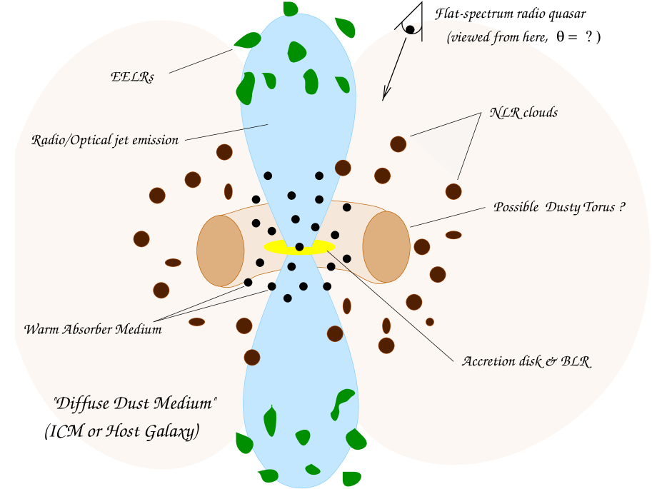
Figure 8.1: Schematic showing possible locations of the dusty medium in Parkes quasars. According to simple unified models for radio-loud AGN, these sources are believed to be observed more-or-less in the direction shown.

Motivated by these results, one can also conduct an an X-ray spectral study to search for signatures of warm absorbers in reddened Parkes quasars. Due to their faintness in the ROSAT energy band however, this may be difficult with existing instruments such as Ginga and ASCA. The high signal-to-noise spectra required may be achieved with the AXAF and XMM satellites.

The Narrow Line Region (NLR)

There is considerable evidence suggesting that the (0.1-1kpc scale ) NLR of AGN contains dust (eg. Wills $et\,al.$ 1993). Netzer & Laor (1993) have shown that if dust absorption is taken into account, the narrow line emission implies covering factors $\raisebox{-3.01385pt}{\mbox{$\stackrel{{\scriptstyle\textstyle>}}{{\sim}}$}}30\%$ for the NLR gas. Photoionization modelling and line intensity ratios suggest low to moderately low optical depths ($A_{V}\sim 0.1-1$) to the central AGN. Emission line ratios provide the most powerful diagnostic for detecting dust in the NLR. Draine & Bahcall (1981) present an exhaustive list of line pairs to measure dust extinction in AGN. If lines of different ionization state and/or velocity width can be used as a distance indicator from the photoionizing continuum source, then line ratios can also be used to constrain the spatial dust distribution.

The profiles of narrow emission lines can also provide a useful diagnostic. The narrow line spectra of Seyfert galaxies, and to a lesser extent high redshift quasars often exhibit lines showing some degree of asymmetry. Both ‘redward’ (excess red flux) and ‘blueward’ asymmetries are found (eg. Boroson & Green, 1992). These are interpreted as due to a combination of net radial motion of the clouds and some extended source of opacity such as dust. The observed asymmetries imply modest extinctions $A_{V}\sim 1$. Correlations with other reddening indicators may also constrain the dust distribution.

Our existing optical spectra are not of sufficient high signal-to-noise and resolution to detect any narrow lines favourable for the above diagnostics. A high resolution spectral study of just a few reddened Parkes quasars will provide vital clues as to whether reddening by NLR dust is important.

Extended Emission Line Regions (EELRs)

Many radio-loud AGN show extended line emission on scales from 1kpc to hundreds of kpc, often cospatial with radio and optical jets (Baum & Heckman, 1989). The line emitting gas is distributed rather inhomogeneously and is likely to be an extension of the smaller scale NLR. Its coincidence with the radio morphology and larger than usual velocity widths suggests that shock heating by non-thermal radio plasma also plays a rôle. A recent study of the EELRs of a number of nearby radio galaxies has found evidence for dust mixed in with the gas (Villar-Martín & Binette, 1996). This was inferred from the relative faintness and absence of (dust sensitive) calcium lines, suggesting severe depletion onto grains.

If flat spectrum radio-quasars are interpreted as sources with radio jets pointing more-or-less along the line-of-sight, then it is possible that our line-of-sight to the central AGN intercepts a large fraction of dusty EELR gas. A large number of Parkes quasars show resolved radio structure on arcsecond scales to millijansky flux levels. An obvious test would then be to look for spatially extended line emission on scales coincident with radio morphologies. Optically thin dust cospatial with this emission would produce a diffuse halo from scattering of line and continuum radiation into the line-of-sight. This project would be possible with the recent emergence of high quality Fabry-Perot etalons for high resolution imaging spectroscopy. The capabilities of HST however would be necessary for narrow line imaging of higher redshift quasars.

8.2.3 Some Theoretical Considerations

The presence of dust physically associated with flat-spectrum radio quasars also raises a number of theoretical issues: What is its origin? Is it external (eg. from a cooling flow), or does it originate from the ISM of the host galaxy? What are its implications for chemical evolution of the associated gas and hence star formation history? How does it interact with the radiation field and plasma in jets and associated shocks? Does it provide an efficient cooling mechanism and a means of transporting angular momentum from the central engine? These latter issues could be explored through simulations of (relativistic) jets in a dusty medium.

Is radiation pressure from the primary continuum source effective in dispersing grains to large scales? This will depend on whether grains are strongly coupled to magnetic fields or gas, or concentrated in gas clouds so that the inward gravitational force of the central black hole will dominate over radiation pressure. For gravity to dominate, grains may have to be embedded in massive and hence optically-thick clouds to avoid ejection from the nuclear region. This would be inconsistent with the requirement of an ‘optically-thin’ medium in Parkes quasars. If these sources are indeed enshrouded by a dust ‘cocoon’ on large enough scales, then the observed SEDs of jets from optical to soft X-ray energies are likely to be modified. Current models of the high frequency SEDs of BL-Lacs would thus need to be revised.

8.2.4 Reddened Radio-Quiet quasars?

On the basis of a dichotomy in the ratio of optical to radio emission, over 80% of optically-selected QSOs are classified as radio-‘quiet’. If the diversity in continuum slopes in Parkes quasars is not an intrinsic property of the sources but due to reddening by dust, then it is quite plausible that radio-quiets are also reddened by comparable amounts of dust. The narrow range in continuum slopes observed for optically-selected QSOs suggests that existing bright optical surveys may be severely incomplete. The observed spread in continuum slopes of Parkes quasars predicts an incompleteness of least 50% in a typical QSO survey of magnitude limit $B_{J}\sim 19$.

How can a reddened population of radio-quiet quasars be detected? Since the extinction implied by reddening in Parkes quasars is relatively ‘low’, this population need not comprise the ultraluminous IRAS galaxies (and type-2 AGN) believed to contain buried, heavily obscured quasars. Surveys at wavelengths where no or little bias against dust obscuration would be optimal. Optical identifications of hard ($\raisebox{-3.01385pt}{\mbox{$\stackrel{{\scriptstyle\textstyle>}}{{\sim}}$}}10$keV) X-ray selected samples which are known to contain a high fraction of extragalactic objects and quasars would be promising. However, the recent emergence of large format, high quality CCDs and multi-object fibre spectrographs such as 2dF on the AAT will provide the necessary technology to search for faint (possibly reddened) quasars.

8.3 Summary

This thesis has studied the problem of incompleteness in optical quasar surveys due to obscuration by dust. This was primarily explored using optical and near-infrared observations of a large complete sample of radio-selected quasars. I have developed simple models and novel techniques to explain the properties of these sources in the framework of a number of absorption and emission mechanisms. Previously unknown correlations between spectral properties were predicted, and some identified observationally. These I hope will provide powerful diagnostics for constraining quasar models in future. Amongst the mechanisms believed to operate in radio-loud quasars, the data strongly suggests that a substantial number are reddened optically by several magnitudes of dust extinction, mostly in their environs. To determine whether radio-quiet quasars have similar amounts of dust in their line-of-sight will require much observational work. This study has substantial room for expansion and should further improve our knowledge of the nature and distribution of quasars.

Appendix A References

ABBREVIATIONS

A&A	Astronomy & Astrophysics
A&ASuppl	Astronomy & Astrophysics Supplements
A&ARv	Astronomy & Astrophysics Review
AJ	Astronomical Journal
ApJ	Astrophysical Journal
Ap&SS	Astrophysics & Space Science
ApJS	Astrophysical Journal Supplements
ARA&A	Annual Review of Astronomy and Astrophysics
BAAS	Bulletin of the American Astronomical Society
Fund. Cos. Phys.	Fundamentals of Cosmic Physics
Lick Obs. Bull.	Lick Observatory Bulletin
Lund Obs. Not.	Lund Observatory Notices
MNRAS	Monthly Notices of the Royal Astronomical Society
PASA	Publications of the Astronomical Society of Australia
PASP	Publications of the Astronomical Society of the Pacific
P&SS	Physics & Space Science
Phys. Lett. B	Physics Letters B
Phys. Rep.	Physics Reports
Rep. Prog. Phys.	Reports & Progress in Physics
Rev. Mod. Phys.	Reviews of Modern Physics

Allamandola,L.J., Tielans,A.G.G.M. & Barker,J.R., 1985. ApJ, 290, 25.

Allen,S.W., 1995. MNRAS, 276, 947.

Angel,J.R.P. & Stockman,H.S., 1980. ARA&A, 18, 321.

Antonucci,R. & Miller,J.S., 1985. ApJ, 297, 621.

Antonucci,R., 1993. MNRAS, 31, 473.

Awaki,H., Koyama,K., Kunieda,H. & Tawara,Y., 1990. Nature, 346, 544.

Babul,A. & Rees,M.J., 1992. MNRAS, 255, 346.

Bahcall,J.N., Kirhakos,S., Saxe,D.H. & Schneider,D.P., 1995. ApJ, 479, 642.

Ballard,K.R., Mead,A.R.G., Brand,P.W.J.L., Hough,J.H., Bailey,J.A. & Brindle,C., 1988. in BL Lac Objects, Proceedings: Como, Italy, p.181.

Bartelmann,M. & Schneider,P., 1993. A&A, 268, 1.

Bartelmann,M., Schneider,P. & Hasinger,G., 1994. A&A, 290, 399.

Barvainis,R., 1987. ApJ, 320, 537.

Barvainis,R., 1993. ApJ, 412, 513.

Baum,S.A. & Heckman,T.M., 1989. ApJ, 336, 702.

Beichman,C.A., Pravdo,S.H., Neugebauer,G., Soifer,B.T., Matthews,K. & Wooten,A.A., 1981. ApJ, 247, 780.

Bergeron,J. & Boisse,P., 1991. A&A, 243, 344.

Björnsson,C. & Blumenthal,G.R., 1982. ApJ, 259, 805.

Blain,A.W. & Longair,M.S., 1993a. MNRAS, 264, 509.

Blain,A.W. & Longair,M.S., 1993b. MNRAS, 265, L21.

Blandford,R.D. & Rees,M.J., 1978. in Pittsburgh Conf. on BL-Lac Objects, ed. A.M. Wolf (Pittsburgh: Univ. Pittsburgh, Dept. of Physics and Astronomy), p.328.

Blandford,R.D. & Kochanek,C.S., 1987. in Dark Matter in the Universe, eds. J.Bahcall,T.Piran & S.Weinberg, p.133.

Blandford,R.D. & Eichler,D., 1987. Phys. Rep., 154, 1.

Blandford,R.D. & Königl,A., 1979. ApJ, 232, 34.

Blumenthal,G.R. & Gould,R.J., 1970. Rev. Mod. Phys., 42, 237.

Bogart,R.S. & Wagoner,R.V., 1973. ApJ, 181, 609.

Bohlin,R.C., Savage,B.D. & Drake,J.F., 1978. ApJ, 224, 291.

Boroson,T.A. & Green,R.F., 1992. ApJS, 80, 109.

Bouchet,P., Lequeux,J., Maurice,E., Prévot,L. & Prévot-Burnichon,M.L., 1985. A&A, 149, 330.

Boyle,B.J., Fong,R. & Shanks,T., 1988. MNRAS, 231, 897.

Boyle,B.J., Shanks,T. & Peterson,B.A., 1988. MNRAS, 235, 935.

Boyle,B.J., Fong,R., Shanks,T. & Peterson,B.A., 1990. MNRAS, 243, 1.

Boyle,B.J. & di Matteo,T., 1995. MNRAS, 277, L63.

Brandt,W.N., Fabian,A.C. & Pounds,K.A., 1996. MNRAS, 278, 326.

Bregman,J.N., Lebofsky,M.J., Aller,M.F., Rieke,G.H., Aller,H.D., Hodge,P.E., Glassgold,A.E. & Huggins,P.J., 1981. Nature, 293, 714.

Bregman,J.N. $et\,al.$ , 1986. ApJ, 301, 708.

Brindle,C., Hough,J.H., Bailey,J.A., Axon,D.J. & Hyland,A.R., 1986. MNRAS, 221, 739.

Bruzual,G. & Charlot,S., 1993. ApJ, 405, 538.

Burbidge,E.M. & Strittmatter,P.A., 1972. ApJ, 174, L57.

Byun,Y.I., 1993. PASP, 105, 993.

Calzetti,D., Kinney,A.L. & Storchi-Bergmann, T., 1994. ApJ, 429, 582.

Canizares,C.R. & White,J.L., 1989. ApJ, 339, 27.

Chang,C.A., Schiano,A.V.R. & Wolfe,A.M., 1987. ApJ, 322, 180.

Cheney,J.B. & Rowan-Robinson,M., 1981. MNRAS, 195, 831.

Chini,R., Krügel,E., Kreysa,E. & Gemund,H.P., 1989. A&A, 216, L5.

Chini,R. & Krügel,E., 1994. A&A, 288, L33.

Ciliegi,P., Elvis,M. Wilkes,B.J. Boyle,B.J, McMahon,R.G. & Maccacaro,T., 1995. MNRAS, 277, 1463.

Clayton,G.C., Martin,P.G. & Thompson,I., 1983. ApJ, 265, 194.

Cotton,W.D., 1983. ApJ, 271, 51.

Cohen,M.H. & Vermeulen,R.C., 1992. in Proc. Conf. on Extragalctic Radio Sources–From Beams to Jets, ed. E. Feigelson, Paris:Inst. d’Astrophys.

Crampton,D. (Editor), 1991. in the Space Distribution of Quasars, ASP Conf. series, vol.21.

Cruz-Gonzalez,I. & Huchra,J.P., 1984. AJ, 89, 441.

De Zotti,G., Franceschini,A., Mazzei,P., Toffolatti,L. & Danese,L., 1995. P&SS, 43, 1439.

Dickman,R.L., 1978. ApJS, 37, 407.

Disney,M., Davies,J. & Phillipps.S., 1989. MNRAS, 239, 939.

Djorgovski,S., Thompson,D. & Smith,J.D., 1993. in First light in the Universe: Stars or QSOs? p.67, ed. B. Rocca-Volmerange, M. Dennefeld, B. Guiderdoni & J. Tran Thanh Van, Gif-sur-Yvette: Editions Frontieres.

Dopita,M.A., 1995. Ap&SS, 233, 215.

Draine,B.T. & Salpeter,E.E., 1979a. ApJ, 231, 77.

Draine,B.T. & Salpeter,E.E., 1979b. ApJ, 231, 438.

Draine,B.T., 1981. ApJ, 245, 880.

Draine,B.T. & Bahcall,J.N., 1981. ApJ, 250, 579.

Draine,B.T. & Lee,H.M., 1984. ApJ, 285, 89.

Draine,B.T., 1985. ApJS, 57, 587.

Drinkwater,M.J., Webster,R.L. & Thomas,P.A., 1993. AJ, 106, 848.

Drinkwater,M.J., Webster,R.L., Francis,P.J., Condon,J.J., Ellison,S.L., Jauncey,D.L., Lovell,J., Peterson,B.A. & Savage,A., 1997. MNRAS, 284, 85.

Drinkwater,M.J., Combes,F. & Wiklind,T., 1996. A&A, 312, 771.

Drury,L.O., 1983. Rep. Prog. Phys., 46, 973.

Duncan,R.A., White,G.L., Wark,R., Reynolds,J.E., Jauncey,D.L., Norris,R.P., Taafe,L. & Savage,A., 1993. PASA, 10, 310.

Dunlop,J.S., Peacock,J.A., Savage,A., Lilly,S.J., Heasley,J.N. & Simon,A.J.B., 1989. MNRAS, 238, 1171.

Dunlop,J.S., Guiderdoni,B., Rocca-Volmerange,B., Peacock,J.A. & Longair,M.S, 1989. MNRAS, 240, 257.

Dunlop,J.S. & Peacock,J.A., 1990. MNRAS, 247, 19.

Dwek,E., Rephaeli,Y. & Mather,J.C., 1990. ApJ, 350, 104.

Eales,S.A. & Rawlings,S., 1993. ApJ, 411, 67.

Edelson,R.A., Malkan,M.A. & Rieke,G.H., 1986. ApJ, 321, 233.

Edelson,R.A. & Malkan,M.A., 1987. ApJ, 323, 516.

Edmunds, M.G., 1990. MNRAS, 246, 678.

Efstathiou,G., Ellis,R.S. & Peterson,B.A., 1988. MNRAS, 232, 431.

Elvis,M., Fiore,F., Wilkes,B. & McDowell,J., 1994. ApJ, 422, 60.

Elvis,M., Wilkes,B., McDowell,J., Green,R.F., Bechtold,J., Willner,S.P., Oey,M.S., Polomski,E. & Cutri,R., 1994. ApJS, 95, 1.

Elvius,A., 1978. Ap&SS, 55, 49.

Fabian,A.C., Nulsen, P.E.J. & Canizares,C.R., 1991. A&ARv, 2, 191.

Fall,S.M., Pei,Y.C. & McMahon, R.G., 1989. ApJ, 341, L5.

Fall,S.M. & Pei,Y.C., 1989. ApJ, 337, 7.

Fall,S.M. & Pei,Y.C., 1993. ApJ, 402, 479.

Fall,S.M. & Pei,Y.C., 1995. in QSO Absorption Lines, ed: G.Meylan, Berlin: Springer-Verlag.

Ferland,G.J. & Netzer,H., 1983. ApJ, 264, 105.

Fireman,E.L., 1974. ApJ, 187, 57.

Fitzpatrik,E.L. & Massa,D., 1990. ApJS, 72, 163.

Franceschini, A., Mazzei P. & De Zotti G., 1994. ApJ, 427, 140.

Francis,P.J., Hewett,P.C., Foltz,C.B., Chaffee,F.H., Weymann,R.J. & Morris,S.L., 1991. ApJ, 373, 465.

Francis,P.J., 1996. PASA, 13, 212.

Francis,P.J., Webster,R.L., Drinkwater,M.J., Masci,F.J. & Peterson,B.A., 1997.            MNRAS, in press.

Freeman, K.C., 1970. ApJ, 160, 811.

Fritz,K.D., 1989a. A&A, 214, 14.

Fritz,K.D., 1989b. ApJ, 347, 692.

Giovanelli,R., Haynes,M.P., Salzer,J.J., Wegner,G., Da Costa,L.N. & Freudling,W., 1994. AJ, 107, 2036.

Glazebrook,K., Peacock,J.A., Miller,L. & Collins,C.A., 1995. MNRAS, 275, 169.

Goudfrooij,P. & de Jong,T., 1995. A&A, 298, 784.

Goudfrooij,P., de Jong,T., Hansen,L. & Nørgaard-Nielsen,H.U., 1994a. MNRAS, 271, 833.

Goudfrooij,P., Hansen,L., Jorgensen,H.E. & Nørgaard-Nielsen,H.U., 1994b. A&ASuppl, 105, 341.

Green,P.J., Schartel,N., Anderson,S.F., Hewett,P.C., Foltz,C.B., Brinkmann,W., Fink,H. Trümper,J. & Margon,B., 1995. ApJ, 450, 51.

Greenberg,J.M., 1968. in Nebulae & Interstellar Matter, Stars and Stellar systems Vol. VII, eds. B.M. Middlehurst & L.H. Aller,, University of Chicago Press. p.221.

Greenberg,J.M., 1971. A&A, 12, 240.

Guiderdoni,B. & Rocca-Volmerange,B., 1987. A&A, 186, 1.

Hartwick,F.D.A. & Schade,D., 1990. ARA&A, 28, 437.

Katz,N., Quinn,T., Bertschinger,E. & Gelb,J.M., 1994. MNRAS, 270, L71.

Heavens,A.F. & Meisenheimer,K., 1987. MNRAS, 225, 335.

Heiles,C., 1987. in Interstellar Processes, eds. D. Hollenbach, H. Thronson, Reidel,Dordrecht, p.171.

Heisler,J. & Ostriker,J.P., 1988. ApJ, 332, 543.

Hewett,P.C., Foltz,C.B & Chaffee,F.H., 1995. ApJ, 109, 1498.

Hill,G.J., Wynn-Williams,C.G. & Becklin,E.E., 1987. ApJ, 316, L11.

Hines,D.C. & Wills,B.J., 1992. BAAS, 24, 1184.

Holman,B.A., 1997. MSc Thesis, The University of Melbourne, Ch.2.

Holmberg,E., 1958. Lund Obs. Not., 2, 136.

Hough,J.H., Bailey,J.A., Rouse,M.F. & Whittet,D.C.B., 1987. MNRAS, 227, 1.

Hoyle,F. & Wickramasinghe,N.C., 1991. The Theory of Cosmic Grains, ed. R.L.F. Boyd et al., Kluwer.

Hu,E.M., Cowie,L.L. & Wang,Z., 1985. ApJS, 59, 447.

Hu,E.M., 1992. ApJ, 391, 608.

Hutchings,J.B. & Morris,S.L., 1995. AJ, 109, 1541.

Impey,C.D. & Neugebauer,G., 1988. AJ, 95, 307.

Impey,C.D. & Tapia,S., 1990. ApJ, 354, 124.

Jansen,R.A., Knappen,J.H., Beckman,J.E., Peletier,R.F. & Hes,R., 1994. MNRAS, 270, 373.

Jones,T.W., Rudnick,L., Owen,F.N., Puschell,J.J., Ennis,D.J. & Werner,M.W., 1981. ApJ, 243, 97.

Kellerman,K.I., 1966. ApJ, 146, 621.

Kellerman,K.I. & Pauliny-Toth,I.I.K., 1969. ApJ, 155, L71.

Kellerman,K.I. & Pauliny-Toth,I.I.K., 1981. ARA&A, 19, 373.

Kirk,J.G. & Schneider,P., 1987. ApJ, 322, 256.

Knapen,J.H., Hes,R., Beckman,J.E. & Peletier,R.F., 1991. A&A, 241, 42.

Kollgaard,R.I., Feigelson,E.D., Laurent-Muehleisen,S.A., Spinrad,H., Dey,A. & Brinkmann,W., 1995. ApJ, 449, 61.

Komossa,S. & Fink,H., 1997. A&A, in press, astro-ph/9707003.

Königl,A., 1981. ApJ, 243, 700.

Kormendy,J., 1992. in Testing the AGN Paradigm, ed. S.S.Holt, S.G.Neff, C.M.Urry, College Park,MD,p.23.

Kriss,G.A. & Canizares,C.R., 1985. ApJ, 297, 177.

Kruper,J.S. & Canizares,C.R., 1989. ApJ, 343, 66.

La Franca,F., Franceschini,A. Cristiani,S. & Vio,R., 1995. A&A, 299, 19.

Landau,R., Golisch,B., Jones,T.J., Jones,T.W., Pedelty,J., Rudnick,L., Sitko,M.L., Kenney,J., Roellig,T., Salonen,E., Urpo,S., Schmidt,G., Neugebauer,G., Mathews,K., Elias,J.H., Impey,C., Clegg,P., Harris,S., 1986. ApJ, 308, 78.

Lanzetta,K.M., 1991. ApJ, 375, 1.

Lanzetta,K.M., Wolfe,A.M. & Turnshek,D.A., 1995. ApJ, 440, 435.

Laor,A. & Draine,B.T., 1993. ApJ, 402, 441.

Ledden,J.E. & O’Dell,S.L., 1983. ApJ, 270, 434.

Ledden,J.E. & O’Dell,S.L., 1985. ApJ, 298, 630.

Lees,J.F., Knapp,G.R., Rupen,M.P. & Phillips,T.G., 1991. ApJ, 379, 177.

Lilly,S.J. & Cowie,L.L, 1987. In Infrared Astronomy with Arrays, eds. C.G. Wynn-Williams & E.E.Becklin, p.473.

Loeb,A., 1993. ApJ, 403, 542.

Longair,M.S., 1993. in The Physics of Background Radiation, Springer Verlag; SAAS-FEE lecture No.23, p.83.

Lonsdale,C.J., Smith,H.E. & Lonsdale,C.J, 1995. ApJ, 438, 632.

Loveday,J., Peterson,B.A., Efstathiou,G. & Maddox,S.J., 1992. ApJ, 390, 338.

Low,F.J., Cutri,R.M., Kleinmann,S.G. & Huchra,J.P., 1989. ApJ, 340, 1.

Lynden-Bell,D., 1969. Nature, 223, 690.

MacAlpine,G.M., 1985. in Astrophysics of Active Galaxies and Quasi-Stellar Objects, , ed. J.S. Miller (Mill Valley:Univ. Science books), p.259.

Madejski,G.M., Mushotzky,R.F., Weaver,K.A. & Arnaud,K.A., 1991. ApJ, 370, 198.

Margolis,S.H. & Schramm,D.N., 1977. ApJ, 214, 339.

Markkanen,T., 1979. A&A, 74, 201.

Martin,P.G., 1970. MNRAS, 149, 221.

Martin,P.G., 1978. Cosmic Dust, Oxford, Clarendon Press.

Masci,F.J. & Webster,R.L., 1995. PASA, 12, 146.

Mather,J.C. $et\,al.$ , 1990. ApJ, 354, L37.

Mathis,J.S., Rumpl,W. & Nordsiek,K.H., 1977. ApJ, 217, 425.

Mathis,J.S., 1986. ApJ, 308, 281.

Mathis,J.S., 1990. ARA&A, 28, 37.

Mathur,S., Wilkes,B., Elvis,M. & Fiore,F., 1994. BAAS, 184, 1706.

McAlary,C.W. & Rieke,G.H., 1988. ApJ, 331, 1.

McCarthy,P.J., 1993. ARA&A, 31, 639.

McDowell,J.C., 1986. MNRAS, 223, 763.

McDowell,J.C., Elvis,M., Wilkes,B.J., Willner,S.P., Oey,M.S., Polomski,E., Bechtold,J. & Green,R.F., 1989. ApJ, 345, L13.

McKee,C.F. & Petrosian, V., 1974. ApJ, 189, 17.

McKee,C.F., Hollenbach,D.J., Seab,C.B. & Tielens,A.G.G.M., 1987. ApJ, 318, 674.

McMahon,R.G., Omont,A., Bergeron,J., Kreysa,E. & Haslam,C.G.T., 1994. MNRAS, 267, L9.

Meisenheimer,K., Röser,H.J., Hiltner,P., Yates,M.G., Longair,M.S., Chini,R. & Perley,R.A., 1989. A&A, 219, 63.

Meyer,D.M., Welty,D.E. & York,D.G., 1989. ApJ, 343, L37.

Meyer,D.M. & Roth,K.C., 1990. ApJ, 363, 57.

Møller,P. & Jacobsen,P., 1990. A&A, 228, 299.

Moore,R.L. & Stockman,H.S., 1984. ApJ, 279, 465.

Morris,S.L. $et\,al.$ , 1991. AJ, 102, 1627.

Morrison,R. & McCammon,D., 1983. ApJ, 270, 119.

Miller,J.S., French,H.B. & Hawley,S.A., 1978. in Pittsburgh Conf. on BL-Lac Objects, ed. A.M. Wolf (Pittsburgh: Univ. Pittsburgh Dept. of Physics and Astronomy), p.176.

Mulchaey,J.S., Mushotzky,R.F. & Weaver,K.A., 1992. ApJ, 390, L69.

Nath,B.B. & Trentham,N., 1997. MNRAS, in press, astro-ph/9707177.

Netzer,H., 1990. in Active Galactic Nuclei, Saas-Fee Advanced Course 20, Springer, Berlin.

Netzer,H. & Laor,A., 1993. ApJ, 404, L51.

Neugebauer,G., Oke,J.B., Becklin,E.E. & Matthews,K., 1979. ApJ, 230, 79.

O’Dell, S.L., 1979. in Active Galactic Nuclei, eds: Hazard, C. & Mitton, S., 1979, p.95.

O’Dell,S.L., Scott,A. & Stein,W.A., 1987. ApJ, 313, 164.

Oey,M.S. & Kennicutt Jr,R.C., 1993. ApJ, 411, 137.

Olive,K.A., Schramm,D.N., Steigman,G. & Walker,T.P., 1990. Phys.Lett.B, 236, 454.

Orr,M.J.L. & Browne,I.W.A., 1982. MNRAS, 200, 1067.

Osterbrock,D.E., 1989. in Astrophysics of Gaseous Nebulae and Active Galactic Nuclei, University Science Books, Mill Valley California, p.326.

Ostriker,J.P. & Heisler,J., 1984. ApJ, 278, 1.

Ostriker,J.P., Vogeley,M.S. & York,D.G., 1990. ApJ, 364, 405.

Pacholczyk,A.G., 1970. in Radio Astrophysics, San Francisco, Freeman.

Padovani,P. & Urry,C.M., 1992. ApJ, 387, 449.

Page,M.J., Carrera,F.J., Hasinger,G., Mason,K.O., McMahon,R.G., Mittaz,J.P.D., Barcons,X., Carballo,R., Gonzalez-Serrano,I. & Perez-Fournon,I., 1996. MNRAS, 281, 579.

Pan,H.C., Stewart,G.C. & Pounds,K.A., 1990. MNRAS, 242, 177.

Peacock,J.A. & Wall,J.V., 1981. MNRAS, 194, 331.

Peebles, P.J.E., 1989. in The Epoch of Galaxy Formation, ed. C.S. Frenk $et\,al.$ (Dordrecht: Kluwer), p.1.

Pei,Y.C., Fall,S.M. & Bechtold,J., 1991. ApJ, 378, 6.

Pei,Y.C., 1992. ApJ, 395, 130.

Pei,Y.C. & Fall,S.M., 1995. ApJ, 454, 69.

Peletier,R.F., Valentijn,E.A., Moorwood,A.F.M., Freudling,W., Knapen,J.H. & Beckman,J.E., 1995. A&A, 300, L1.

Pettini,M., Boksenberg,A. & Hunstead,R.W., 1990. ApJ, 348, 48.

Pettini,M., Smith,L.J., Hunstead,R.W. & King,D.L., 1994. ApJ, 426, 79.

Pettini,M., King,D.L., Smith,L.J. & Hunstead,R.W., 1997. ApJ, 478, 536.

Phillipps,S., 1986. ApJ, 25, L19.

Pier,E.A. & Krolik,J.H., 1992. ApJ, 401, 99.

Pier,E.A. & Krolik,J.H., 1993. ApJ, 418, 673.

Press,W.H., Teukolsky,S.A., Vetterling,W.T., Flannery,B.P., 1994. Numerical Recipes in C, 2nd edition, Cambridge University Press, p.547.

Puchnarewicz,E.M., Mason,K.0., Romero-Colmenero,E., Carrera,F.J., Hasinger,G. McMahon,R., Mittaz,J.P.D., Page,M.J. & Carballo,R., 1996. MNRAS, 281, 1243.

Rao,S. & Briggs,F.H., 1993. ApJ, 419, 515.

Readhead,A.C.S., 1994. ApJ, 426, 51.

Rees,M.J., 1990. Science, 247, 817.

Reynolds,C.S. & Fabian,A.C., 1995. MNRAS, 273, 1167.

Reynolds,C.S., 1996. MNRAS, 286, 513.

Rieke,M. & Lebofsky,M.J., 1979. ARA&A, 17, 477.

Rieke,G.H., Lebofsky,M.J. & Kinman,T.D., 1979. ApJ, 232, L151.

Rieke,G.H., 1982. In Extragalactic radio sources; (Proceedings, Albuquerque Symposium), Dordrecht, p.239.

Rieke,G.H., Lebofsky,M.J. & Wiśniewski,W.Z., 1982. ApJ, 263, 73.

Rieke,M. & Lebofsky,M.J., 1985. ApJ, 288, 618.

Rix,H.W. & Rieke,M., 1993. ApJ, 418, 123.

Rocca-Volmerange,B. & Guiderdoni,B., 1987. A&ASuppl, 74, 185.

Rodrigues-Williams,L.L. & Hogan,C.J., 1994. AJ, 107, 451.

Rodrigues-Williams,L.L. & Hawkins,C.J., 1995. Proc, of the 5th Annual Astrophysics Conference, Maryland.

Romani,R.W. & Maoz,D., 1992. ApJ, 386, 36.

ROSAT Users’ Handbook, 1994. Edited by U.G. Briel $et\,al.$ , Max-Planck-Institut für extraterrestriche Physik, http://heasarc.gsfc.nasa.gov/docs /rosat/ruh/handbook/handbook.html.

Rudnicki,K., 1986. in Proc. Internat. of Physics “Enrico Fermi”, Summer School, 86, 480.

Sandage,A., 1972. ApJ, 178, 25.

Sanders,D.B., soifer,B.T., Elias,J.H., Neugebauer,G. & Matthews,K., 1988. ApJ, 328, L35.

Sanders,D.B., Phinney,E.S.,Neugebauer,G.,Soifer,B.T. & Matthews,K., 1989. ApJ, 347, 29.

Sarazin,C.L., 1986. Rev. Mod. Phys., 58, 1.

Sargent,W.L.W., Boksenberg,A. & Steidel,C.C., 1988. ApJS, 68, 539.

Saunders,W., Rowan-Robinson,M., Lawrence,A., Efstathiou,G., Kaiser,N., Ellis,R.S. & Frenk,C.S., 1990. MNRAS, 242, 318.

Savage,B.D. & Mathis,J.S., 1979. ARA&A, 17, 73.

Savaglio,S., D’Odorico,S., & Möller,P., 1994. A&A, 281, 331.

Schartel,N., Green,P.J., Anderson,S.F., Hewett,P.C., Foltz,C.B., Margon,B., Brinkmann,W., Fink,H. & Trümper,J., 1996. MNRAS, 283, 1015.

Schmidt,M. & Green,R.F., 1983. ApJ, 269, 352.

Schmidt,M. Schneider,D.P. & Gunn,J.E., 1988. in Optical Surveys for Quasars, (ed. P.S. Osmer, A.S. Porter, R.F. Green, C.B. Foltz, Provo: Brigham Young Univ. Press), p.87.

Scoville,N. & Norman,C., 1988. ApJ, 332, 163.

Searle,L., 1971. ApJ, 168, 327.

Seaton,M.J., 1979. MNRAS, 187, 73.

Seitz,S. & Schneider,P., 1995. A&A, 302, 9.

Serjeant,S. & Rawlings,S., 1996. Nature, 379, 304.

Serkowski,K., Mathewson,D.E. & Ford,V., 1975. ApJ, 196, 261.

Shuder,J.M., 1981. ApJ, 244, 12.

Siebert,J. $et\,al.$ 1997. A&A, in preparation.

Sitko,M.L. & Zhu,Y., 1991. ApJ, 369, 106.

Smith,E.P. & Heckman,T.M., 1989. ApJ, 341, 658.

Smith,P.S., Balonek,T.J., Heckert,P.A. & Elston,R., 1986. ApJ, 305, 484.

Soifer,B.T., Houck,J.R. & Neugebauer,G., 1986. ARA&A, 25, 187.

Songaila,A. & Cowie,L.L., 1996. AJ, 112, 335.

Songaila,A., 1997. ApJ, in press, astro-ph/9709046.

Spinrad,H. & Smith,H.E., 1975. ApJ, 201, 275.

Spinrad,H. & Djorgovski,S., 1987. in Proc. IAU Symp. No. 126, ed: G.Burbidge, p.129.

Stebbins,J., Huffer,C.H. & Whitford,A.E., 1934. Publ. Washburn Obs., 15, part V.

Stickel,M., Fried,J.W. & Kühr,H., 1993. A&ASuppl, 98, 393.

Stocke,J.T., Morris,S.L., Gioia,I.M., Maccacaro,T. & Schild,R., 1991. ApJS, 76, 813.

Stockman,H.S., Moore,R.L. & Angel,J.R.P., 1984. ApJ, 279, 485.

Takeda,H., Nulsen,P.E.J. & Fabian,A.C., 1984. MNRAS, 208, 261.

Taylor,G.L., Dunlop,J.S., Hughes,D.H. & Robson,E.I., 1996. MNRAS, 283, 930.

Teräsranta,H. & Valtaoja,E., 1994. A&A, 283, 51.

Thomas,P.A. & Webster,R.L., 1990. ApJ, 349, 437.

Tinsley,B.M., 1976. ApJ, 208, 797.

Tinsley,B.M., 1980. Fund. Cos. Phys., 5, 287.

Trumpler,R.J., 1930. Lick Obs. Bull., 114, 154.

Tytler,D., Boksenberg,A., Sargent,W.L.W. & Kunth,D., 1987. ApJS, 64, 667.

Ulrich,M., 1988. in Conference on BL Lac Objects (Como, Italy), eds: L.Maraschi, T.Maccacaro, M.Ulrich, p.45.

Urry,C.M. & Padovani,P., 1995. PASP, 107, 803.

Valentijn,E.A., 1990. Nature, 346, 153.

Valentijn,E.A., 1994. MNRAS, 206, 614.

Véron-Cetty,M.P. & Véron, 1989. A Catalogue of Quasars and Active Nuclei, 4th Edition, Munich: ESO.

Vila-Costas,M.B. & Edmunds,M., 1992. MNRAS, 259, 121.

Villar-Martín,M. & Binette,L., 1997. A&A, 317, 350.

Visnovsky,K.L., Impey,C.D., Foltz,C.B., Hewitt,P.C., Weymann,R.J. & Morris, S.L., 1992. ApJ, 391, 560.

Wall,J.V. & Peacock,J.A., 1985. MNRAS, 216, 173.

Wang,B., 1991a. ApJ, 374, 456.

Wang,B., 1991b. ApJ, 383, L37.

Warren,S.J. Hewett,P.C. & Osmer,P.S., 1994. ApJ, 421, 412.

Webster,R.L., Francis,P.J., Peterson,B.A., Drinkwater,M.J. & Masci,F.J., 1995. Nature, 375, 469.

Weinberg,S., 1972. Gravitation and Cosmology: Principles and Applications of the General Theory of Relativity, New York, Wiley.

Wheeler,J.C., Snedin, C. & Truran,J.W., 1989. ARA&A, 27, 279.

White,S.D.M. & Frenk,C.S., 1991. ApJ, 379, 52.

Whittet,D.C.B. & van Breda,I.G., 1978. A&A, 66, 57.

Whittet,D.C.B., 1992. Dust in the Galactic Environment, eds. R. Tayler, R. White, Cambridge University Press.

Whittet,D.C.B., Martin,P.G., Hough,J.H., Rouse,M.F., Bailey,J.A. & Axon,D.J., 1992. ApJ, 386, 562.

Wilkes,B.J., Wright,A.E., Jauncey,D.L. & Peterson,B.A., 1983. PASA, 5, 2.

Wilkes,B.J., 1986. MNRAS, 218, 331.

Wilkes,B.J. & Elvis,M., 1987. ApJ, 323, 243.

Wilkes,B.J., Elvis,M., Fiore,F., McDowell,J.C., Tananbaum, H. & Lawrence,A., 1992. ApJ, 393, L1.

Wilkes,B.J., Tananbaum,H., Worrall,D.M., Avni,Y., Oey,M.S. & Flanagan,J., 1994. ApJS, 92, 53.

Wilking,B.A., Lebofsky,M.J. & Rieke,G.H., 1982. AJ, 87, 695.

Wills,B.J., 1988. in BL-Lac Objects, Proc. Como, Italy, eds. L. Maraschi, T. Maccacaro, p.114.

Wills,B.J., Wills,D., Evans,N.J.I., Natta,A., Thompson,K.L., Breger,M. & Sitko,M.L., 1992. ApJ, 400, 96.

Wills,B.J., Wills,D., Breger,M., Antonucci,R.R.J. & Barvainis,R., 1992. ApJ, 398, 454.

Wills,B.J., Netzer,H., Brotherton,M.S., Mingsheng Han, Wills,D. Baldwin,J.A., Ferland,G.J. & Browne,I.W.A., 1993. ApJ, 410, 534.

Wise,M.W., O’Connell,R.W., Bregman,J.N. & Roberts,M.S., 1993. ApJ, 405, 94.

Wolfe,A.M., Turnshek,D.A., Smith,H.E. & Cohen,R.D., 1986. ApJS, 61, 249.

Womble,D.S., Sargent,W.L.W. & Lyons,R.S., 1996. in Cold Gas at High Redshift, eds. M. Bremer, H. Rottgering, P. van der Werf, C. Carilli, (Kluwer).

Wright,A.E., Ables,J.G. & Allen,D.A., 1983. MNRAS, 205, 793.

Wright,E.L., 1986. ApJ, 311, 156.

Wright,E.L., 1990. ApJ, 353, 411.

Xu,C. & Buat,V., 1995. A&A, 293, 65.

Yee,H.K. & Oke,J.B., 1978. ApJ, 226, 753.

Zaritsky,D., 1994. AJ, 108, 1619.

Zaritsky,D., Kennicutt,R.C., Jr. & Huchra,J.P., 1994. ApJ, 420, 87.

Appendix B Cosmology

“Everything should be made as simple as possible, but not simpler.”

— Albert Einstein, 1879-1955

In this thesis, we have assumed the Friedmann-Lemaître cosmological model. This is based on a spatially homogeneous and isotropic universe with $\Lambda=0$. All calculations use a deceleration parameter $q_{0}=0.5$ ($\Omega=1$) and a Hubble parameter of $H_{0}=50\,\rm km\,s^{-1}\,Mpc^{-1}$, unless otherwise stated. In cases where $h_{50}$ and $h_{100}$ are used, these are defined via $H_{0}=50h_{50}$ and $H_{0}=100h_{100}\,\rm km\,s^{-1}\,Mpc^{-1}$ respectively.

Below are some relations used throughout this thesis to transform between apparent and physical quantities of interest. For a brief derivation, see Weinberg (1972).

The apparent angular size of a source, $\theta^{\prime\prime}$, in terms of its physical diameter $r$ is given by:

$$\theta\,=\,\frac{(2.06\times 10^{5})(1+z)^{2}\,r}{D_{L}}{\rm\hskip 14.22636ptarcsec},$$ (B.1)

where $D_{L}$ is the luminosity distance defined as

$$D_{L}\,=\,\frac{c}{H_{0}}q_{0}^{-2}\left[1-q_{0}+q_{0}z+(q_{0}-1)(1+2q_{0}z)^{1/2}\right].$$ (B.2)

$\frac{c}{H_{0}}$ is the Hubble distance ($\equiv 6.05\times 10^{9}\,h_{50}^{-1}$pc).

To transform luminosity functions into properties that are directly observable such as magnitude and redshift distributions, we need a specification of the evolutionary and $k$-correction for the sources under consideration. The evolutionary correction is a quantity defining the physical evolution in source luminosity as a function of redshift. The $k$-correction is due to sampling of the rest frame SED at different portions through a fixed observational bandpass as it is redshifted. Both of these are defined in magnitudes.

Absolute and apparent magnitudes are related by

$$M\,=\,m-5\log d_{L}-43.88+5\log h_{50}-e(z)-k(z)$$ (B.3)

where $e(z)$ and $k(z)$ are respectively the evolutionary and $k$-correction corresponding to the bandpass in which $m$ is measured as defined above. In Eqn. B.3, $d_{L}$ is the luminosity distance in units of $c/H_{0}$ (ie. $d_{L}\equiv(H_{0}/c)D_{L}$ with $D_{L}$ from Eqn. B.2).

The number counts of sources as a function of apparent magnitude is an integral of the luminosity function $\phi$ over all redshifts. In general, the number of sources per unit apparent magnitude per square degree of sky can be written

$$N(m)\,=\,\int^{z_{max}}_{z_{min}}dz\,\left(\frac{dV}{dz}\right)\phi(M,z),$$ (B.4)

where $dV/dz$ is the comoving volume element per square degree of sky and $m$ is the apparent magnitude corresponding to the absolute magnitude $M$. In the standard Friedmann cosmology, the comoving volume element per square degree of sky is

$$\frac{dV}{dz}\,=\,6.5\times 10^{7}h_{50}^{-3}(1+z)^{3}(1+2q_{0}z)^{-1/2}d_{L}^{2}\,\,{\rm\,deg^{-2}Mpc^{3}}.$$ (B.5)

The redshift distribution, or number of sources per unit redshift, per square degree of sky contributing to some apparent magnitude interval $m_{min}<m<m_{max}$ is given by

$$n(z)\,=\,\frac{dV}{dz}\int^{M(m_{max})}_{M(m_{min})}dM\,\phi(M,z).$$ (B.6)

Appendix C Derivations in Evolutionary Dust Model

Here we derive exact expressions for the mean and variance in total optical depth in galactic dust as a function of redshift in our evolutionary dust model of Chapter 4. The scaling of these quantities with model parameters was defined by Eqns. 4.12 and 4.14. The galaxies are modelled as exponential dusty disks, randomly inclined to the line-of-sight.

We first derive the average number of galaxies intercepted by a light ray emitted from some redshift $z$ (ie. Eqn. 4.11). Given a ‘proper’ number density of galaxies at some redshift $n_{g}(z)$, with each galaxy having an effective cross-sectional area $\mu\,\sigma$ as viewed by an observer ($\mu$ is a random inclination factor, where $\mu=\cos\,\theta$ and $\theta$ is the angle between the sky plane and the plane of a galactic disk), then the average number of intersections of a light ray along some path length $ds$ will be given by

$$dN\,=\,n_{g}(z)\,\mu\sigma\,ds.$$ (C.1)

In an expanding universe we have $n_{g}=n_{0}(1+z)^{3}$, where $n_{0}$ is a local comoving number density and is assumed to be constant. Units of proper length and redshift are related by

$${ds\over dz}\,=\,\left({c\over H_{0}}\right)\,{1\over(1+z)^{2}(1+2q_{0}z)^{1/2}}$$ (C.2)

(Weinberg, 1972). The effective cross-section projected towards an observer for a randomly inclined disk is found by averaging over the random inclination factor $\mu$, where $\mu$ is randomly distributed between 0 and 1 and integrating over the exponential profile assumed for each disk with scale radius $r_{0}(z)$ (see Eqns. 4.1 and 4.9). The product $\mu\sigma$ in Eqn. C.1 is thus replaced by

$$\int_{0}^{1}\mu\,d\mu\,\int_{0}^{\infty}e^{-r/r_{0}(z)}\,2\pi r\,dr\,=\,\pi\,{r_{0}}^{2}(1+z)^{2\delta}.$$ (C.3)

Thus from Eqn. C.1, the average number of intersections up to some redshift $z$ is given by

$$\bar{N}(z)\,=\,\int_{0}^{z}\mu\sigma\,n_{g}(z^{\prime})\,\left({ds\over dz^{\prime}}\right)\,dz^{\prime}$$

$$=\,n_{0}\pi r_{0}^{2}\left({c\over H_{0}}\right)\int_{0}^{z}{(1+z^{\prime})^{1+2\delta}\over(1+2q_{0}z^{\prime})^{1/2}}\,dz^{\prime}.$$ (C.4)

With $\tau_{g}$ being defined by $n_{0}\pi r_{0}^{2}\left({c\over H_{0}}\right)$, this directly leads to Eqn. 4.11 for $q_{0}=0.5$.

The mean optical depth $\bar{\tau}$ is derived by a similar argument. If $\tau_{0}(z)$ is the optical depth observed through a face on galaxy at some redshift $z$ (Eqn. 4.8), then a galactic disk inclined by some factor $\mu$ will have its optical depth increased to $\tau_{0}(z)/\mu$. Multiplying this quantity by Eqn. C.1, the extinction suffered by a light ray along a path length $ds$ is given by

$$d\tau\,=\,n_{g}(z)\,\sigma\,\tau_{0}(z)\,ds.$$ (C.5)

Thus the mean optical depth to some redshift $z$ can be calculated from

$$\bar{\tau}(z)\,=\,\int_{0}^{z}\sigma n_{g}(z^{\prime})\tau_{0}(z^{\prime})\left({ds\over dz^{\prime}}\right)\,dz^{\prime}.$$ (C.6)

Given $n_{g}(z)$, $\left({ds\over dz}\right)$ and $\sigma$ (from the integral over $r$ in Eqn. C.3) above, and $\tau_{0}(z^{\prime})$ from Eqn. 4.8, the mean optical depth follows the general form

$$\bar{\tau}(z)\,=\,2\tau_{g}\tau_{B}\int_{0}^{z}{(1+z^{\prime})^{2.5+2\delta}\over(1+2q_{0}z^{\prime})^{1/2}}\,\left[1-{\ln(1+z^{\prime})\over\ln(1+z_{dust})}\right]\,dz^{\prime}.$$ (C.7)

Similarly, the variance in the optical depth distribution is defined as the following

$$\sigma_{\tau}^{2}(z)\,=\,\langle\tau^{2}\rangle-{\langle\tau\rangle}^{2}\,=\,\int_{0}^{z}\sigma n_{g}(z^{\prime}){\tau_{0}}^{2}(z^{\prime})\left({ds\over dz^{\prime}}\right)\,dz^{\prime}.$$ (C.8)

In terms of our model dependent parameters, this becomes

$$\sigma_{\tau}^{2}(z)\,=\,2\tau_{g}{\tau_{B}}^{2}\int_{0}^{z}{(1+z^{\prime})^{4+2\delta}\over(1+2q_{0}z^{\prime})^{1/2}}\,{\left[1-{\ln(1+z^{\prime})\over\ln(1+z_{dust})}\right]}^{2}\,dz^{\prime}.$$ (C.9)

That it will never come again,
Is what makes life so sweet.

— Emily Dickinson, Poem Number 1741