Role of the scalar field in gravitational lensing

Abstract

A static and circularly symmetric lens characterized by mass and scalar charge parameters is constructed. For the small values of the scalar charge to the mass ratio, the gravitational lensing is qualitatively similar to the case of the Schwarzschild lens; however, for large values of this ratio the lensing characteristics are significantly different. The main features are the existence of two or nil Einstein ring(s) and a radial critical curve, formation of two or four images and possibility of detecting three images near the lens for sources located at relatively large angular positions. Such a novel lens may also be treated as a naked singularity lens.

1 Introduction

The deflection of light in a gravitational field predicted by the general theory of relativity witnessed experimental verification in 1919. The spectacular phenomena resulting from the deflection of light in a gravitational field are referred to as the gravitational lensing (GL). Chwolson, in 1924, pointed out that if a background star (source), a deflector (gravitational lens) and an observer are perfectly aligned, a ring-shaped image of the source centered on the deflector would appear (see in Schneider et al. 1992). This is, however, usually called as the ‘Einstein Ring’. Einstein (1936) obtained the apparent luminosities of the images of a star (source) due to a foreground star (gravitational lens). He mentioned that if the source, the lens and the observer are sufficiently aligned, the images will be highly magnified. However, arguing that the angular image splitting caused by a stellar-mass lens is too small to be resolved by an optical telescope, and we shall scarcely ever approach close enough to an alignment with the source and the deflector, he remarked that there is a little chance to observe lensing phenomena caused by stellar-mass lenses. Though several authors (Eddington 1920, Chwolson 1924) discussed that the deflection of light in a gravitational field may give rise to GL, only Zwicky (1937a,b) expressed his vision clearly that the observation of the GL phenomena would be a certainty. The studies of GL remained in almost a dormant stage until Klimov, Liebes and Refsdal independently re-opened this subject with their pioneering work in 1960’s . Klimov (1963) investigated the lensing of galaxies by galaxies, whereas Liebes (1964) studied lensing of stars by stars and also stars by globular clusters in our galaxy. Refsdal (1964a,b) was the first to argue that the geometrical optics can be used in studying the properties of point-mass gravitational lenses and the time delay resulting from the lensing phenomena.

A quasar is an ideal source for GL because of its high luminosity, point-like appearance, prominent spectral features and the large distance from the earth (high probability of deflectors intervening the source and the observer). The great vision of Zwicky became true when Walsh, Carswell and Weymann discovered the first example of the GL - the QSO 0957+561 A,B (Walsh et al. 1979). The two images of a single QSO were separated by six $arcseconds$. Both images had similar optical spectra, a galaxy was found between the images, the flux ratio between images was found to be the same in the optical as well as in the radio wavebands, and VLBI observations showed detailed correspondence between various knots in the two radio images (cf. Narasimha et al. 1984, Narayan and Bartelmann 1996). The VLBI features were modelled by Narasimha et al. (1984) who demonstrated that a cluster in addition to the giant elliptical was needed for producing the observed features. Following this landmark discovery, more than a dozen confirmed examples of multiply- imaged quasars are known and, in addition, six ring-shaped radio images have been found (Refsdal and Surdej 1994, Keeton and Kochanek 1995). The Einstein rings for extended sources were predicted by Saslaw et al. (1985) and were first discovered by Hewitt et al. (1987). The detection of new lensing phenomena, namely giant luminous arcs and arclets, and microlensing events have increased dramatically in recent years. For a review on giant luminous arcs and arclets see Fort and Miller(1994) and on microlensing see Narasimha (1995) and Roulet and Mollerch (1997). Cheng and Refsdal (1979, 1984) as well as Subramanian et al. (1985) developed the theory of microlensing to explain the flux variability in the images. The traditional dynamical method to obtain masses of celestial bodies in the universe requires that the system under investigation is in dynamical equilibrium. Therefore, this method has limitation in its use. However, there are no such restrictions to the use of GL and therefore, in recent years, it has become the most important tool for probing the universe. Indeed Narasimha and Chitre (1989) predicted that dark extended massive objects could act as lenses for systems like 2345+007, MG 2016+112 etc. which was confirmed with the discovery of a dark but X-ray bright cluster at redshift of 1 in the system MG 2016+112 by Hattori et al. (1997). Narasimha (1994) discussed the gravitational lens as a probe of dark matter in the universe. The GL can give important informations on masses of galaxies, the composition of dark matter, cosmological parameters, existence of exotic massive objects, the large scale structure of the universe and can be also used to test the alternative theories of gravitation. A gravitational lens provides a highly magnified view of the distant objects in the universe and therefore acts as a cosmic telescope. Since the last decade the GL has become one of the most important research fields in cosmology (Schneider et al. 1992, Refsdal and Surdej 1994, Narayan and Bartelmann 1996, Wu 1996).

The GL is very likely to serve an important tool to detect exotic objects in the universe, such as cosmic strings and there have been attempts to investigate if any of the confirmed gravitational lenses could be due to the action of cosmic strings (see Hogan and Narayan 1984, Vilenkin 1984, 1986, Gott 1985, de Laix and Vachaspati 1996 and references therein). There is no compelling evidence that any of the observed gravitational lenses are due to a cosmic string. However, it is essential to develop new gravitational lens models with objects which are though not yet observed, are not forbidden on theoretical grounds. It is well-known that the scalar fields have been conjectured (since before the outset of the general theory of relativity) to give rise to the long-range gravitational fields, and several theories involving scalar fields have been proposed (see Abraham 1914, Bergmann 1956, Brans and Dicke 1961, Callan et al. 1970, Garfinkle et al. 1991, 1992, Yilmaz 1992, Horne and Horowitz 1992, 1993 and references therein). The scalar fields minimally as well as conformally coupled to gravitation have been a subject of active theoretical research. In recent years, there is a growing interest in the studies of scalar (dilaton) fields, because of their importance in string theories. There have been a number of studies of light propagation in the unconventional scalar-tensor theories of gravity (Sanders 1989, Bekenstein and Sanders 1994 and references therein). However, the problem of formation of critical curves and consequent appearance of multiple images has not received adequate attention. In the present paper we study the effects of the massless scalar field on the Schwarzschild lensing. More precisely, we build a new static and circularly symmetric singular lens model characterized by two parameters: the Schwarzschild mass and the “scalar charge”. For this purpose we take the most general static spherically symmetric asymptotically flat exact solution to the Einstein-Massless Scalar (EMS) equations, given by Janis, Newman and Winicour (JNW) (Janis et al. 1968). Wyman (1981) obtained a static spherically symmetric exact solution to the EMS equations and later Roberts (1993) showed that the most general static spherically symmetric solution to the EMS equations (with zero cosmological constant) is asymptotically flat and this is the Wyman solution. The Wyman solution is well considered in the literature. Recently one of us (Virbhadra 1997) showed that the Wyman solution is the same as the JNW solution, which was obtained about thirteen years ago, we therefore call it the JNW solution. Switching off the “scalar charge” in this solution one recovers the well-known Schwarzschild solution. Hereafter, we will refer to the new lens model as the Schwarzschild-Massless Scalar (SMS) lens. For small values of the ratio of the “scalar charge” to the Schwarzschild mass, the SMS lensing does not have any new qualitative (though differs quantitatively) features and resembles the Schwarzschild lensing phenomena. However, for reasonably large value of this ratio, the Einstein deflection angle starts with a negative value, becomes positive, reaches a maximum and then decreases to zero as the closest distance of approach increases from a small value to the infinity. This behaviour of the SMS lens gives rise to few interesting features, for instance, it gives radial critical curves (radial caustics in the source plane) and concentric Einstein double rings (tangential caustics in the source plane). These effects are not found in any of the known singular lens models. Moreover, the number of images also differs from the case of the Schwarzschild lensing. It is worth mentioning that the JNW solution has a strong curvature globally naked singularity (Virbhadra et al. 1997). It is not known how one would be able to distinguish observationally black holes from naked singularities (if these exist). Our present investigations reveal the qualitative different features and consequently the results we present here could be useful in differentiating between the two kinds of objects. The rest of the paper is organized as follows: In Sect. 2, we derive the Einstein deflection angle for a general static and spherically symmetric metric, which generalizes the result obtained by Weinberg (1972). Sect. 3 discusses the JNW solution for obtaining the deflection angle for this case. In Sect. 4 we obtain positions of images, magnification, and tangential and radial critical curves and in Sect. 5 we discuss possible observational tests. In the last Section we summarize the qualitative features of the lens. We follow the convention that Latin indices take values $0\ldots 3$ and use geometrized units, for instance $M\equiv GM/c^{2}$.

2 Einstein deflection angle for a general static spherically symmetric metric

We consider a general static and spherically symmetric spacetime given by the line element

$$ds^{2}=B\left(r\right)dt^{2}-A\left(r\right)dr^{2}-D\left(r\right)r^{2}\left(d\vartheta^{2}+\sin^{2}\vartheta\ d\phi^{2}\right).$$ (1)

The null geodesics equations are

$$\frac{dv^{i}}{dk}+\Gamma^{i}_{jk}v^{j}v^{k}=0,$$ (2)

where

$$g_{ij}v^{i}v^{j}=0.$$ (3)

$v^{i}\equiv\frac{dx^{i}}{dk}$ is the tangent vector to the null geodesics. $k$ is the affine parameter.

Eqs. $(2)$ with Eq.$(1)$ give

$$B\frac{dt}{dk}=K,$$ (4)

$$Dr^{2}\sin^{2}\vartheta\frac{d\phi}{dk}=J,$$ (5)

$$\frac{d^{2}\vartheta}{dk^{2}}+\left(\frac{2}{r}+\frac{D^{\prime}}{D}\right)\frac{dr}{dk}\frac{d\vartheta}{dk}-\sin\vartheta\cos\vartheta{\left(\frac{d\phi}{dk}\right)}^{2}=0,$$ (6)

and

$$\frac{d^{2}r}{dk^{2}}+\frac{A^{\prime}}{2A}\left(\frac{dr}{dk}\right)^{2}-\frac{D^{\prime}r^{2}+2Dr}{2A}\left[\left(\frac{d\vartheta}{dk}\right)^{2}+\sin^{2}\vartheta\left(\frac{d\phi}{dk}\right)^{2}\right]+\frac{B^{\prime}}{2A}\left(\frac{dt}{dk}\right)^{2}=0.$$ (7)

$K$ and $J$ are constants of integrations. The prime denotes the derivative with respect to the coordinate $r$. Without loss of generality we take

$$\frac{dt}{dk}=\frac{1}{B}.$$ (8)

Appealing to the spherically symmetric nature of the metric under consideration we consider the geodesics, without loss of generality, on the equatorial plane ($\vartheta=\pi/2$). Following Weinberg (1972, Chapters 8.4 and 8.5), we get the equation for the photon trajectories as

$$\phi(r)-\phi_{\infty}={\int_{r}}^{\infty}\left(\frac{A(r)}{D(r)}\right)^{1/2}\left[\left(\frac{r}{r_{0}}\right)^{2}\frac{D(r)}{D(r_{0})}\frac{B(r_{0})}{B(r)}-1\right]^{-1/2}\ \frac{dr}{r},$$ (9)

where $r_{0}$ is the closest distance of approach. The integration constant $J$ is

$$J=r_{o}\sqrt{\frac{D(r_{o})}{B(r_{o})}}.$$ (10)

The Einstein deflection angle is given by

$$\hat{\alpha}\left(r_{0}\right)=2|\phi\left(r_{0}\right)-\phi_{\infty}|-\pi,$$ (11)

where $\phi\left(r_{0}\right)-\phi_{\infty}$ is read through the Eq. $(9)$. The above expression reduces to the result obtained by Weinberg (1972) if one takes $D=1$.

3 Janis-Newman-Winicour solution and the deflection angle

There have been some studies of bending of light in scalar-tensor theories (Bekenstein and Sanders 1994). We wish to consider a gravitational lens endowed with the conventional mass and a “scalar charge”, described by the JNW solution. We now discuss the JNW solution in order to derive the Einstein deflection angle for the JNW metric. The Einstein-Massless Scalar equations (EMS) are

$$R_{ij}\ -\ \frac{1}{2}\ R\ g_{ij}\ =\ 8\pi\ S_{ij}\ ,$$ (12)

where $S_{ij}$, the energy-momentum tensor of the massless scalar field, is given by

$$S_{ij}\ =\ \Phi_{,i}\ \Phi_{,j}\ -\ \frac{1}{2}\ g_{ij}\ g^{ab}\ \Phi_{,a}\ \Phi_{,b}\ ,$$ (13)

and

$$\Phi_{,i}^{\ ;i}\ =\ 0.$$ (14)

$\Phi$ stands for the massless scalar field. The comma and semicolon before indices denote the partial and covariant derivatives, respectively. $R_{ij}$ is the Ricci tensor and $R$ is the Ricci scalar. Eq. $(12)$ with Eq. $(13)$ can be expressed as

$$R_{ij}\ =\ 8\pi\ \Phi_{,i}\ \Phi_{,j}.$$ (15)

JNW obtained the most general static spherically symmetric asymptotically flat exact solution to the EMS equations, which is given by the line element (cf. Virbhadra 1997)

$$ds^{2}=\left(1-\frac{b}{r}\right)^{\gamma}dt^{2}-\left(1-\frac{b}{r}\right)^{-\gamma}dr^{2}-\left(1-\frac{b}{r}\right)^{1-\gamma}r^{2}\left(d\vartheta^{2}\ +\ \sin^{2}\vartheta\ d\phi^{2}\right)$$ (16)

and the scalar field

$$\Phi=\frac{q}{b\sqrt{4\pi}}\ln\left(1-\frac{b}{r}\right),$$ (17)

where

$$\gamma = \frac{2M}{b},$$

$$b = 2\sqrt{M^{2}+q^{2}}.$$ (18)

Note that $b<r<\infty$, and $b$ is the curvature singularity; $M$ and $q$ are constant parameters which represent the total mass and the “scalar charge” respectively. Clearly $q=0$ recovers the Schwarzschild solution. The “scalar charge” does not contribute to the total mass of the system, but it does affect the curvature of the spacetime (Virbhadra 1997). The JNW solution can be used in two ways: first, it describes the exterior gravitational field of an object whose radius is greater than the parameter $b$ in the solution. Second, it describes the field due a naked singularity (Virbhadra et al. 1997). Comparing Eq. $(1)$ with Eq. $(16)$, one has for the JNW solution

$$B = A^{-1}=\left(1-\frac{b}{r}\right)^{\gamma},$$

$$D = \left(1-\frac{b}{r}\right)^{1-\gamma}.$$ (19)

Substituting the above in Eq. $(11)$, one gets the Einstein deflection angle

$$\hat{\alpha}\left(r_{0}\right)=2\ {\int_{r_{0}}}^{\infty}\frac{dr}{r\sqrt{1-\frac{b}{r}}\ \sqrt{\left(\frac{r}{r_{0}}\right)^{2}\left(1-\frac{b}{r}\right)^{1-2\gamma}\left(1-\frac{b}{r_{0}}\right)^{2\gamma-1}-1}}-\pi.$$ (20)

Introducing dimensionless parameters

$$x=\frac{r}{b},$$

$$x_{0}=\frac{r_{0}}{b},$$ (21)

one can re-write the expression for the deflection angle

$$\hat{\alpha}\left(x_{0}\right)=2\ {\int_{x_{0}}}^{\infty}\frac{dx}{x\sqrt{1-\frac{1}{x}}\ \sqrt{\left(\frac{x}{x_{0}}\right)^{2}\left(1-\frac{1}{x}\right)^{1-2\gamma}\left(1-\frac{1}{x_{0}}\right)^{2\gamma-1}-1}}-\pi$$ (22)

The integral in the above is defined for $x_{0}>(2\gamma+1)/2$. For the Schwarzschild metric ($\gamma=1$) this gives $r_{0}>3M$. The first derivative of the deflection angle is given by

$$\hat{\alpha}^{\prime}\left(x_{0}\right)=\frac{2\gamma+1-2x_{0}}{{x_{0}}^{2}\left(1-\frac{1}{x_{0}}\right)}{\int_{x_{0}}}^{\infty}\frac{\left(4\gamma x-2\gamma-1\right)dx}{\left(2\gamma+1-2x\right)^{2}\ x\ \sqrt{1-\frac{1}{x}}\ \sqrt{\left(\frac{x}{x_{0}}\right)^{2}\left(1-\frac{1}{x}\right)^{1-2\gamma}\left(1-\frac{1}{x_{0}}\right)^{2\gamma-1}-1}}.$$ (23)

After lengthy, but straightforward calculations Eq. ($20$) gives the Einstein deflection angle (up to the second order) as follows.

$$\hat{\alpha}\left(r_{0}\right)=\frac{4M}{r_{0}}+\frac{4M^{2}}{{r_{0}}^{2}}\left(\frac{15\pi}{16}-2\right)+\frac{2}{{r_{0}}^{2}}\left[2M\sqrt{M^{2}+q^{2}}-\frac{q^{2}\pi}{8}\right]+.....\ \ \ .$$ (24)

We trivially recover the deflection angle for the Schwarzschild lens when $q=0$ in the above equation. The second order term for the Schwarzschild case is obviously positive. In the following section we use equations $(22)$ and $(23)$ to perform computations.

4 Image positions, magnification and critical curves

We have given the lens diagrams in Fig. 1. The first one is applicable to the case when the bending angle is positive and the other one is for the negative deflection. We take the reference axis to be the line from the observer O to the lens L and keep the distance from the deflector to the observer, $D_{ol}$, fixed. An image position is specified by the angle $\theta$ between OL and the tangent to the null geodesic at the observer. The observer is assumed to be located in an asymptotically flat spacetime. A null geodesic through the observer is uniquely specified by the angle $\theta$. The impact parameter is $D_{ol}\sin\theta$ and $D_{ls}$ stands for the distance from the source S to the point C in the lens plane. $D_{os}$ stands for the distance from the observer to the source. $\beta$ denotes the true angular position of the source, whereas $\theta$ stands for the image positions. With these definitions, the lens equation may be expressed as

$$\sin\left(\theta-\beta\right)=\frac{D_{ls}}{D_{os}}\sin\hat{\alpha}.$$ (25)

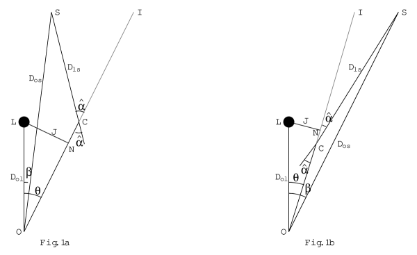
Figure 1: The geometry of a gravitational lens: $S$ is the source location, $O$ is the observer and $L$ is the lens. The angular separations of the source and the image positions from the lens are denoted by $\beta$ and $\theta$, respectively. $\hat{\alpha}$ is the Einstein bending angle. The bending angle is taken to be positive in case ${\bf a}$ where the contribution due to the mass is dominant while it is negative in case ${\bf b}$ where the “scalar charge” contributes more. $D_{os}$ represents the observer-source distance, $D_{ol}$ the observer-lens distance and $D_{ls}$ the lens-source distance. The lines $SC$ and $OI$ are tangents on the null geodesics at $S$ and $O$, respectively.

We define

$$\alpha=\sin^{-1}\left(\frac{D_{ls}}{D_{os}}\sin\hat{\alpha}\right).$$ (26)

From the lens diagram one has

$$\sin\theta=\frac{J}{D_{ol}}.$$ (27)

Using Eqs. $(10),(19),(21),$ and $(27)$ we get

$$\sin\theta=\frac{b}{D_{ol}}\ x_{o}\ \left(1-\frac{1}{x_{o}}\right)^{\frac{1-2\gamma}{2}},$$ (28)

where $b=2q$ for $\gamma=0$ and it is $2M/\gamma$ for $\gamma\neq 0$.

The magnification of images is given by

$$\mu=\left(\frac{\sin{\beta}}{\sin{\theta}}\ \frac{d\beta}{d\theta}\right)^{-1}.$$ (29)

The tangential and radial critical curves follow from the singularities in

$$\mu_{t}\equiv\left(\frac{\sin{\beta}}{\sin{\theta}}\right)^{-1},$$ (30)

and

$$\mu_{r}\equiv\left(\frac{d\beta}{d\theta}\right)^{-1},$$ (31)

respectively. To obtain magnification the first derivative of the deflection angle with respect to $\theta$ is required, which is given by

$$\frac{d\hat{\alpha}}{d\theta}=\hat{\alpha}^{\prime}\left(x_{o}\right)\frac{dx_{o}}{d\theta},$$ (32)

where

$$\frac{dx_{o}}{d\theta}=\frac{2x_{o}\left(1-\frac{1}{x_{o}}\right)^{\frac{2\gamma+1}{2}}\sqrt{1-\left(\frac{b}{D_{ol}}\right)^{2}{x_{o}}^{2}\left(1-\frac{1}{x_{o}}\right)^{1-2\gamma}}}{\frac{b}{D_{ol}}\left(2x_{o}-2\gamma-1\right)}.$$ (33)

Figure 2: The deflection angle $\alpha$ and the angle $\theta-\beta$ are plotted as a function of the angular separation $\theta$ of the image from the lens, indicated by the continuous and dashed lines, respectively. The dotted line passing through the origin represents the source position precisely aligned with the lens ($\beta=0$) and its intersections with the continuous curves give the two Einstein radii. For a specified position of the source the points of intersection of the continuous curves with the dashed line give the image positions. Here $\gamma=0.005$, $D_{ol}=10^{10}M$ and $\beta=\pm 10$. Angles are in arcseconds.

Table 1: Image positions for $\gamma=0.005$

Images on the opposite side of the source		Source position	Images on the same side of the source
$\theta_{outer}$	$\theta_{inner}$	$\beta$	$\theta_{inner}$	$\theta_{outer}$
11$2.5852$	11 $0.1641$	$0.5$	$0.1610$	11 $3.1008$
11$2.3592$	11 $0.1658$	$1.0$	$0.1595$	11 $3.3901$
11$1.8006$	11 $0.1712$	$2.5$	$0.1554$	11 $4.3735$
11$1.1876$	11 $0.1822$	$5.0$	$0.1493$	11 $6.3132$
11$0.8208$	11 $0.1972$	$7.5$	$0.1441$	11 $8.4838$
11$0.5795$	11 $0.2203$	$10.0$	$0.1395$	11 $10.7776$
11$0.3765$	11 $0.2783$	$12.5$	$0.1354$	11 $13.1396$
11No image	11 No image	$15.0$	$0.1317$	11 $15.5418$
11No image	11 No image	$17.5$	$0.1284$	11 $17.9693$
11No image	11 No image	$20.0$	$0.1253$	11 $20.4135$

• We have taken $D_{ol}=10^{10}M$. Angles are in arcseconds.

Figure 3: The magnifications: tangential $\mu_{t}$ denoted by dotted curves, radial $\mu_{r}$ denoted by dashed curves, and total $\mu$ shown as continuous curves are plotted as a function of the image position $\theta$ for $\gamma=0.005$. The singularities of $\mu_{t}$ and $\mu_{r}$ give positions of the tangential and radial critical curves, respectively. Here $D_{ol}=10^{10}M$ and angles are in arcseconds.

To obtain image positions on both sides of the optic axis one plots $\alpha\left(\theta\right),\theta-\beta$ against $\theta$ and $-\alpha\left(\theta\right),-\theta-\beta$ against $-\theta$. The points of intersection give the image positions. The continuous line on the right (left) hand side of the vertical axis is $\alpha\left(\theta\right)$ against $\theta$ (-$\alpha\left(\theta\right)$ against $-\theta$). The dashed lines on the right (left) hand side of the vertical axis are $\theta-\beta$ against $\theta$ ($-\theta-\beta$ against $-\theta$). The dotted lines are, similarly, $\theta$ vs. $\theta$ and $-\theta$ vs. $-\theta$. The intersections of $\alpha\left(\theta\right)$ with $\theta$ give the angular positions of tangential critical curves (Einstein rings). For these computations we have considered $D_{ls}/D_{os}=1/2$ and $D_{ol}=10^{10}M$ (for $\gamma\neq 0$). We have plotted for $\gamma=0.005$ (see Fig. 2). In Table 1, we have given image positions for few values of the source positions for $\gamma=0.005$. In Fig. 3, we have plotted tangential magnification $\mu_{t}$ and radial magnification $\mu_{r}$ against $\theta$ for $\gamma=0.005$. Singularities in these give the positions of tangential critical curves (TCC) and radial critical curves (RCC), respectively. In the same figure we have also plotted total magnification $\mu$ vs. $\theta$. In Table 2, we give the positions of TCC and RCC for few values of $\gamma$.

For $\gamma=0.005$, as shown in Fig. 2, $\alpha$ has large negative value for small $\theta$, becomes positive and then goes to zero (asymptotically) as $\theta$ increases. The dashed lines are for $\beta=\mp 10$ arcseconds. The dotted line ($\beta=0$) cuts the continuous lines at two points on each side of the vertical axis and therefore one gets two concentric Einstein rings. As $\beta$ increases from zero (see the lower part of the figure) the dashed line cuts the continuous curves at four points (two on each side of the vertical axis) giving rise to four images (two images on each side of the optic axis). As $\beta$ increases the two images on the opposite side of the source come closer and eventually meet at the RCC whereas those on the same side of the source get separated. For any further increase in $\beta$ there is no image on the opposite side of the source. In Table 1, we have given image positions for few values of the source positions for $\gamma=0.005$. Out of the two images on the same side of the optic axis, the one which is nearer to the optic axis we call the inner image and the other which is farther from the optic axis we call the outer image. For this particular case we have plotted $\mu_{t}$ and $\mu_{r}$ to identify the TCC and RCC (see Fig. 3). Magnification $\mu$ is also plotted. We have two TCC and one RCC (the RCC lies in between the two TCC). The magnification falls off sharply near the inner TCC as compared to the RCC as well as the outer TCC. For $\gamma=0.001$, $\alpha$ has large negative value for small $\theta$, becomes positive and then goes to zero (asymptotically) as $\theta$ increases. There are two images of opposite parities on the same side of the source. As $|\beta|$ decreases the two images meet at the RCC and for any further decrease in $|\beta|$ there is no image. There is no Einstein ring for this case. For $\gamma\geq 0.5$ the GL is qualitatively similar to the Schwarzschild lensing (one has only one TCC and has two images, one on each side of the optic axis).

We have given the angular positions of critical curves for few values of $\gamma$. $\theta_{t}^{inner},\theta_{r}$ and $\theta_{t}^{outer}$ stand for the angular positions of the inner TCC, RCC, and outer TCC, respectively.

Table 2: Positions of critical curves

$\gamma$	$\Theta_{t}^{(inner)}$	$\Theta_{r}$	$\Theta_{t}^{(outer)}$
$0.001$	No	$3.4159$	No
$0.002$	$1.2326$	$1.5701$	$2.0984$
$0.003$	$0.4616$	$0.8323$	$2.6588$
$0.004$	$0.2551$	$0.4923$	$2.7812$
$0.005$	$0.1625$	$0.3202$	$2.8324$
$0.01$	$0.0405$	$0.0810$	$2.8966$
$0.5$	No	No	$2.9170$
$1.0$	No	No	$2.9171$

• $\theta_{t}^{inner},\theta_{r}$ and $\theta_{t}^{outer}$ stand for the angular positions of the inner tangential curves, radial critical curves, and outer tangential curves , respectively. We have taken $D_{ol}=10^{10}M$ and angles are expressed in arcseconds.

An increase in the “scalar charge” to the mass ratio (decrease in $\gamma$) decreases the value of angular position of the outer TCC and increases the value of the inner TCC and the RCC. The angular separation between the two Einstein rings decreases with the increase in this ratio. For “very large” value of this ratio (for example, for $\gamma\leq 0.001$) there is only RCC and there is no TCC and for the small value of this ratio (for instance, for $\gamma\geq 0.5$) there is only one TCC and no RCC. For “large” value of this ratio (for instance, for $\gamma=0.005,0.01$) there is one RCC, which lies in between two TCC’s. In the entire investigations we have not considered points close to the integral singularities.

5 Gravitational lens as a diagnostic of scalar charge

We have given, in Table 1, typical solutions for the positions of images due to lensing by “scalar charge” and normal mass and have shown the same in Fig. 2. The corresponding critical curves are given in Table 2 and are displayed in Fig. 3. The observations of double Einstein rings near the centres of relativistic star clusters in galactic nuclei could be a powerful probe of “scalar charge”. The most important property of such a configuration useful for the diagnostic of the lens is the formation of four images of a background radio source located at about an arcsecond from the line of sight to the centre of the lens. Two of the images will be at opposite sides of the lens and will be bright, but the other two images (one on each side of the lens) will be generally faint. For a source sufficiently away from the optic axis, two images will be formed, both in the same side of the lens unlike the normal mass distribution acting as lens. The present VLBA and VLBI are capable of detecting the radio images at milliarcseconds and inferring from the spectral characteristics that they could indeed be images of the same background object. The ellipticity of the mass distribution in the lens could alter the image configuration. Still, if we do indeed detect four radio images nearly collinear, it will lend support to possible existence of “scalar charge”. More probable configuration will, of course, be formation of two images on the same side of the lens. Though difficult to detect, if these features should turn out to be present, it could provide a means to determine the relative gravitational influence of the “scalar charge” q and mass M in the lens.

Our results become important if the following observations yield positive results: Observations of relativistic star clusters in galactic nuclei should show evidence for double ring structure or four images of a background source along a line or two images in the same side of the lens with no evidence for a third image in the other side. These results, if found to be true, will strongly argue in favour of existence of “scalar charges” in the universe.

6 Discussion and Summary

The gravitational lens can serve as a very useful tool to discover exotic objects in the universe (described by matter fields which are not detected, as yet) as well as to test alternative theories of gravity. Even before the advent of the general theory of relativity, scalar fields have been proposed to simulate the long-range gravitational fields and it still continues (see in Horne and Horowitz 1992, Yilmaz 1992 and references therein). Bekenstein and Sanders (1994) discussed that gravitational lenses in scalar-tensor theories could be divergent under some circumstances. We studied the null geodesics in a general static spherically symmetric spacetime and calculated the Einstein deflection angle. The deflection angle for a general static spherically symmetric metric obtained in this work can be used to construct circular gravitational lens models (with different matter fields) in the Einstein theory as well as in alternative theories of gravity. We have used this result to study a circularly symmetric gravitational lens in the Einstein-Massless Scalar theory, by considering the most general static and spherically symmetric solution, given by Janis et al. This describes the exterior field due a spherically symmetric massive object endowed with “scalar charge”. The same field also describes the spacetime due to a naked singularity. Though the existence of a naked singularity is debatable, this subject has recently attracted the attention of many researchers’ minds (see Virbhadra et al. 1997 and references therein). It is not altogether clear how one would be able to distinguish observationally a black hole from a naked singularity (if indeed these exist). We propose that the present lens model could be helpful for this purpose.

The new Schwarzschild-Massless Scalar gravitational lens has interesting features which are not shared by other known circularly symmetric gravitational lenses. For “small” values of the “scalar charge” to the mass ratio the lensing is qualitatively similar (but quantitatively different) to the Schwarzschild lens. For these cases, like the Schwarzschild lens, there are two images of opposite parities (one on each side of the optic axis), there exits no radial critical curve, and there is only the Einstein ring. The “scalar charge” contributes to the decrease in the radius of the Einstein ring. However, when the “scalar charge” to the mass ratio is not small, the gravitational lens action is quite different from the Schwarzschild lensing. When this ratio is “very large” (for example, $\gamma\leq 0.001$) one gets two images of opposite parities on the same side of the source or nil depending upon the source position. There exists one radial critical curve and no tangential critical curve (no Einstein ring) in this case. However, for “large” ratio cases there are four images (two on each side of the optic axis) or two on the same side of the source, depending upon the location of source. There exist two tangential critical curves (double Einstein rings) and one radial critical curve which lies in between them. One interesting feature of these cases (“very large” as well as “large” ratio) is that one can get images of positive parity and sometimes large magnification at smaller angles compared to the source position, cf. Table 1. An image which forms at smaller angular position compared to its source position are usually demagnified, unless it is close to a critical curve. Thus, under some situations one can get magnified image at smaller angular position compared to its source position.

- [1] Abraham M., 1914, Jahrb. Radioakt. Electronik 11, 470
- [2] Bekenstein J. D., Sanders R. H., 1994, ApJ 429, 480
- [3] Bergmann O, 1956, Am. J. Phys. 24, 38
- [4] Brans C. H., Dicke R. H., 1961, Phys. Rev. 124, 925
- [5] Callan C. G, Jr., Coleman S., Jackiw R., 1970, Ann. Phys. (N.Y.) 59, 42
- [6] Cheng K., Refsdal S., 1979, Nat 282, 561
- [7] Cheng K., Refsdal S., 1984, A & A 132, 168
- [8] de Laix A. A., Vachaspati T., 1996, Gravitational lensing by cosmic strings loops, astro-ph/9605171
- [9] Eddington A. S., 1920, Space, time and gravitation, Cambridge University Press, Cambridge
- [10] Einstein A., 1936, Sci 84, 506
- [11] Fort B., Miller Y., 1994, A&AR 5, 239
- [12] Garfinkle D, Horowitz G.T., Strominger A., 1991, Phys. Rev. D43, 3140
- [13] Garfinkle D., Horowitz G.T., Strominger A., 1992, Erratum : Phys. Rev. D45, 3888
- [14] Gott III J., R., 1985, ApJ 228, 422
- [15] Hattori M. et al., 1997, Nat. 388, 146
- [16] Hewitt J. N. et al., 1987, ApJ 321, 706
- [17] Hogan C. J., Narayan R., 1984, MNRAS 2111, 575
- [18] Horne J. H., Horowitz G.T., 1992, Phys. Rev. D46, 1340
- [19] Horne J. H., Horowitz G. T., 1993, Nucl. Phys. B399, 169
- [20] Janis A. I., Newman E. T., Winicour J., 1968, Phys. Rev. Lett. 20, 878
- [21] Klimov Yu. G., 1963, Sov. Phys. Doklady 8, 119
- [22] Keeton II C. R., Kochanek C. S., in: Astrophysical Applications of Gravitational Lensing, IAU Symp., 173, eds. C. S. Kochanek and J. N. Hewitt, Kluver, Boston, p419
- [23] Liebes Jr. S., 1964, Phys. Rev. 133, B835
- [24] Narasimha D., Subramanian K., Chitre S. M., 1984, MNRAS 210, 79
- [25] Narasimha D., Chitre S. M., 1989, Astron. J. 97, 327
- [26] Narasimha D., 1994, in: ICNAPP, ed. R. Cowsik, 251
- [27] Narasimha D., 1995, Bull. Astr. Soc. India 23, 489
- [28] Narayan R., Bartelmann M., 1996, Lectures on gravitational lensing, astro-ph/9606001
- [29] Refsdal S., 1964a, MNRAS 128, 295
- [30] Refsdal S., 1964b, MNRAS 128, 307
- [31] Refsdal S., Surdej J., 1994, Rep. Prog. Theor. Phys. 57, 117
- [32] Roberts M. D., 1993, Ap&SS, 200, 331
- [33] Roulet E., Mollerch S., 1997, Phys. Rep. 279, 67
- [34] Sanders, R. H., 1989, MNRAS 241, 135
- [35] Saslaw W C, Narasimha D., Chitre S. M., 1985, ApJ 292, 348
- [36] Schneider P., Ehlers J., Falco E. E., 1992, Gravitational Lenses, Springer Verlag, Berlin
- [37] Subramaniam K., Chitre S. M., Narasimha D., 1985, ApJ 289, 37
- [38] Vilenkin A., 1984, ApJ L51, 282
- [39] Vilenkin A., 1986, Nat. 322, 613
- [40] Virbhadra K. S. , Jhingan S., Joshi P. S., 1997, Int. J. Mod. Phys. D6, 357
- [41] Virbhadra K. S., 1997, Int. J. Mod. Phys. A12, 4831
- [42] Walsh D., Carswell R. F., Weyman R.J., 1979 Nature 279, 381
- [43] Weinberg S., 1972, Gravitation and cosmology: principles and applications of the general theory of relativity, John Wiely & Sons, NY
- [44] Wyman M., 1981, Phys. Rev. D24, 839
- [45] Wu X. P., 1996, Fund. Cosmic Phys. 17, 1
- [46] Yilmaz H., 1992, Il Nuovo Cimento 107B, 941
- [47] Zwicky F., 1937a, Phys. Rev. 51, 290
- [48] Zwicky F., 1937b, Phys. Rev. 51, 679