The Bull’s-Eye Effect as a Probe of $\Omega$

Abstract

We compare the statistical properties of structures normal and transverse to the line of sight which appear in theoretical N-body simulations of structure formation, and seem also to be present in observational data from redshift surveys. We present a statistic which can quantify this effect in a conceptually different way from standard analyses of distortions of the power-spectrum or correlation function. From tests with $N$–body experiments, we argue that this statistic represents a new and potentially powerful diagnostic of the cosmological density parameter, $\Omega$.

1 Introduction

According to the Hubble law, $v\simeq cz\simeq H_{0}d$, the recession velocity $v$ of a galaxy, inferred from its redshift, is proportional to its proper distance from the observer, $d$. Irregularities gravitationally generate peculiar velocities ($v_{p}$), so that the true relationship is $v=H_{0}d+v_{p}$, where $v_{p}$ is the line of sight component of the peculiar motion. Maps of galaxy positions constructed by assuming that velocities are exactly proportional to distance (redshift space) have two principal distortions. The first is generated in dense collapsed structures where there are very many galaxies at essentially the same distance from the observer, each with a random peculiar motion. This results in a radial stretching of the structure known as a “Finger of God”. The second effect acts on much larger scales (e.g. Kaiser 1987). A large overdensity generates coherent bulk motions in the galaxy distribution as it collapses. Material generally flows towards the center of the structure, i.e. towards the observer for material on the far side of the structure and away from the observer on the near side so it will appear compressed along the line of sight. This tends to make voids bigger and the walls between them denser.

One particularly important unresolved issue is the value of the cosmological density parameter, $\Omega$, which determines whether the universe will expand forever ($\Omega<1$), or eventually recollapse ($\Omega>1$). See e.g. Coles and Ellis (1997) for a review. While redshift-space distortions are a nuisance when one wants to construct accurate maps of the (true) spatial distribution of galaxies, they may lead to a robust determination of $\Omega$. Unfortunately, applications of this idea to existing data have so far yielded inconclusive results for $\Omega$ (Hamilton 1998 and references therein) and recent studies indicate that systematic errors in the standard approaches are likely to be less manageable than has previously been supposed (e.g. Hatton & Cole 1997; see also de Laix and Starkman 1997).

We propose here an entirely new approach to the analysis of these distortions, based on the statistics of the spacing of features (Praton & Schneider 1994; Praton, Melott & McKee 1997) both orthogonal and tangential to the observer’s line of sight in redshift space: the “Bull’s-eye Effect.” Praton et al. (1997) showed that preferentially concentric redshift space features emerging in N–body simulations were dynamical in origin with only very small additional contributions from survey geometry or magnitude limits. Simulations with no peculiar velocities or with randomized velocities show no enhanced Bull’s–eye pattern. We show herein a method of quantifying this difference in the redshift direction, which depends on large–scale motions. This approach bypasses much of the bias dependence implicit in the standard methods of analysis, possibly leading to a much cleaner determination of the density parameter $\Omega$. Further, this effect exists independent of the selection function. A selection function may mildly enhance the visual prominence of the effect, but it is created by redshift distortions.

Concentric rings seem to appear in such surveys as Las Campanas (Schectman et. al 1996) and CNOC2 (Yee et al. 1997). We have developed a quantitative method to detect this signal, which is useful in distinguishing between high and low $\Omega$. If peculiar velocities are low, and observed concentric structures are not enhanced in redshift space (as advocated for the Great Wall by Dell’Antonio et. al 1996), this is not a refutation of the Bull’s-Eye effect. It is evidence for low $\Omega$.

2 Dynamics of The Bull’s-Eye Effect

The effect of peculiar motions is to increase the spacing of large–scale structures in the radial direction as compared with real space, as we show quantitatively below. The enhancement is $\Omega$–dependent. It is on the basis of this visually-striking difference between the redshift-space behavior of low-density and high-density dynamics that we propose a statistic that reproduces the eye’s sensitivity to differences in pattern.

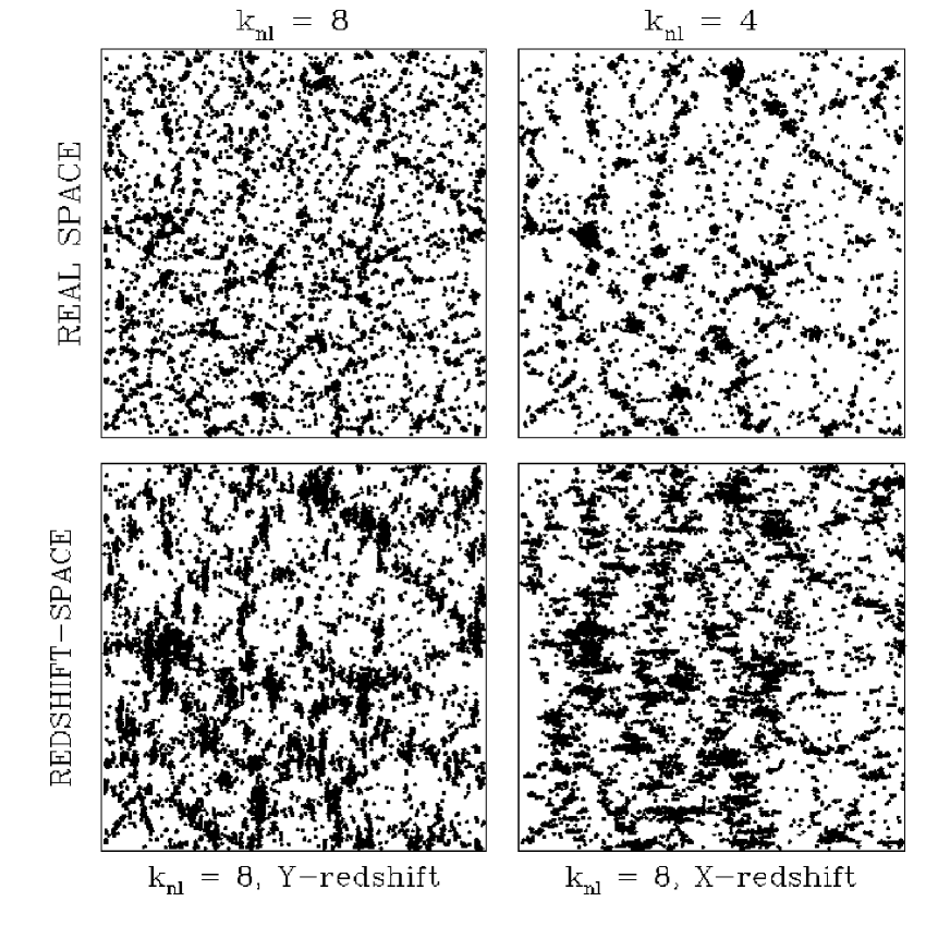
Figure 1: Top-left: a map showing the true positions of all particle positions in a two-dimensional simulation with $\Omega=1$ and an initial power spectrum $P(k)\propto k^{0}$ (corresponding to $n=-1$ in 3D). The top right panel shows the same realization evolved to an expansion factor $a(t)$ twice that of the preceding panel. The bottom two panels show the top-left panel viewed in redshift space using the $y$ and $x$ directions (small angle distant observer approximation). Note the increased spacing between structures along the redshift direction.

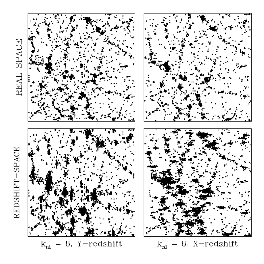
Figure 2: The same as in Figure 1, but for a simulation with $\Omega_{0}$ = 0.2.

It is easier to introduce and explain this effect in the small–angle approximation to redshift space. A distant patch of the Universe will have nearly parallel radii and perpendicular to it circular arc segments of constant $z$. In Figure 1, we show an array of plots from such a Cartesian N–body simulation, described fully in Beacom et. al (1991). Upper left and right represent sequential stages. The two lower plots show the stage at the upper left viewed along its $y$ or $x$ axes in redshift space. There is considerable large–scale displacement in this $\Omega=1$ model, which acts to somewhat anticipate structures that will appear later in real space (upper right). Figure 2 shows the same thing in an $\Omega_{0}=0.2$ simulation. While the “Fingers of God” are still present, the large–scale displacements are largely gone.

The essence of large–scale redshift space effects is a compression and/or expansion effect along the line of sight. It can best be explained using the Zel’dovich approximation (Zel’dovich 1970). This is now known to reproduce weakly non-linear (i.e. large–scale) features in the distribution of matter very accurately indeed, if implemented in an optimized form known as the Truncated Zel’dovich Approximation (Coles et al. 1993, Melott 1994). This approximation follows the development of structure by relating the final (Eulerian) position of a particle ${\bf r}$ at some time $t$ to its initial (Lagrangian) position ${\bf q}$ defined at the primordial epoch when particles were smoothly distributed:

$${\bf r}=a(t){\bf x}({\bf q},t)=a(t)[{\bf q}-D_{+}(t)\nabla_{\bf q}\Phi({\bf q})],$$

where $D_{+}(t)$ describes the linear growth of perturbations as a function of cosmological proper time, $t$, and $a(t)$ is the cosmic scale factor (c.f. Peebles, 1980). In the case of a flat universe, $D_{+}(t)=a(t)$; the behavior of $D_{+}$ for more general cosmologies is usually parameterized by $f=d\log D_{+}/d\log a$, where $f$ can be accurately approximated as $\Omega^{0.6}$.

In the separable mapping (1), the displacement field is given by the gradient of the primordial gravitational potential $\Phi$ with respect to the initial coordinates. Differentiating the expression (1) leads to

$${\bf V}={d{\bf r}\over dt}=H{\bf r}-a(t)\dot{D}_{+}\nabla_{\bf q}\Phi({\bf q})$$

for the velocity of a fluid element ${\bf V}$. The mapping (2) provides a straightforward explanation of the changed characteristic scale of structures in the redshift direction. Calculating the redshift coordinate exactly and translating it into an effective distance $d_{z}$ gives

$$d_{z}={V\over H}=r_{3}-fa(t)D_{+}(t)\nabla_{3}\Phi({\bf q})=aq_{3}-(1+f)a(t)D_{+}(t)\nabla_{3}\Phi({\bf q}),$$

in which we have the 3-axis in the redshift direction. (Note that $\delta$, the density contrast, does not enter here.) Thus the displacement term becomes multiplied by a factor $(1+f)$ in (3) compared to (2).

The effect of the displacement field in redshift space is to give the observer a “preview” (albeit in only one direction) of a later stage of the clustering hierarchy. In effect, the characteristic scale of structures in the z-direction should be larger than that in the directions unaffected by the extra displacements induced by redshift-space distortions. We interpret the characteristic scale as the typical distance between caustics where the mapping (1) becomes singular, which are the prominent high-density features of large-scale structure.

At first sight, this argument seems to suggest that the characteristic the characteristic spacing of high-density regions should be a factor of $(1+f)$ higher for the z-direction than in the orthogonal direction, i.e. a factor of two difference in a critical density universe. The real situation is, however, more complicated than that. The dominant effect of the extra displacements in (3) compared to (1) is their tendency to compress structures together, decreasing their number per unit length and increasing the typical space between them. This effect is, however, contaminated by the Fingers of God, which tend to increase the apparent radial extent of high-density regions and therefore push neighboring structures together, even in low-density universes where the large-scale displacement effect is negligible. The upshot of this is that, for a critical density universe, the effect is rather less than the naive factor of two but, as we shall see, there is still a highly significant difference in characteristic spacings between low– and high–$\Omega$ models.

This effect is rather more subtle than the simple amplification of the power spectrum amplitudes one obtains by applying Eulerian perturbation theory to the problem (Kaiser 1987). The change in pattern from real to redshift space is due to phase changes associated with the extra displacements. These changes do not appear in the power spectrum (which ignores phase information), but are visually clear as they result in the merging of high-density structures and a consequent increase in the spacing between them.

3 Quantifying Displacements

Our method has the character of a first-order statistic (it is related to the mean spacing of objects) rather than the usual second-order statistics (such as the power spectrum), which are blind to the number-density of objects. First, we smooth the distribution in the simulations to produce a continuous density field in order to erase strongly non-linear small-scale structures. We have found empirically that smoothing by a Gaussian $\exp(-r^{2}/\alpha^{2}r_{0}^{2})$ where $r_{0}$ is defined by $\xi(r_{0})=1$ and $\alpha=0.5$ gives the best results, with weak sensitivity to smoothing scale. We then construct density contours for the smoothed field, and take lines-of-sight through the smoothed density field and calculate the rms distance between successive up-crossings of the same contour level in the radial direction; denoted $S_{\parallel}$. Note that there will be one down-crossing of the same level between any two successive up-crossings. Since it is our intention to capture caustics, we concentrate on high-density contours. In fact, we found that for a variety of $\Omega$ and power spectral values, the most reliable approach is to choose a contour level by specifying the filling factor of regions above the contour, not an absolute $\delta$, and that the level corresponding to a filling factor of 15%, about the peak of the spacing, is an excellent choice.

We also do a similar calculation for tangential lines (in the direction orthogonal to the observer’s line of sight); this is denoted $S_{\perp}$. After much experimentation with a large ensemble of simulations, one statistic turned out to be nearly optimal: the ratio of the rms spacing in the redshift direction to that in the orthogonal direction, which we call $\mu$:

$$\mu={S_{\parallel}\over S_{\perp}}$$

We verified that $\mu$ is independent of the power spectrum, and amount of nonlinearity, for a given background cosmology. We tested a total of 16 different high resolution 2d simulations – four realizations each, power law spectra $P(k)\propto k^{2}$, or constant, in both low (0.2) and high ($\Omega=1$) models. The rms spacing for an $\Omega=1$ universe is larger in the redshift direction than in the direction orthogonal to the line of sight. As $\Omega_{0}\rightarrow 0$, the ratio decreases.

In Figure 3a, we show the rms distances $S$ as a function of filling factor. Boldface denotes those measured in the redshift direction, light the orthogonal one; low $\Omega_{0}$ is dashed, high $\Omega$ has solid lines. It is clear that redshift space intervals are larger than real space ones. (We defer showing error bars to 3b, to avoid a crowded plot.) Is the ratio $\Omega$–dependent? We show $\mu$ in 3b, with one-$\sigma$ errors in the mean obtained by averaging over all lines of sight in an ensemble of N-body simulations. These errors are typically larger than the measurement and systematic errors of the redshift. It is clear that $\mu$ is much larger in a critical density Universe–at about a 4$\sigma$ confidence level.

We have also performed a preliminary analysis of a pair of large (256³) simulations with a CDM-type power spectrum in a low– and critical–density background. In these simulations we have used the spherical symmetry that would be seen by a real observer, rather than the simplified Cartesian redshift space shown in the Figures for illustration. However, a full study of this type will require a variety of analyses with varying initial power spectra, amplitudes, survey geometries and magnitude limits which is beyond the scope of this Letter.

4 Discussion

We have described a new statistic for extracting estimates of $\Omega$ from redshift space distortions. We demonstrated that this method is very sensitive to the choice of $\Omega$. We have described its dynamical origin, and showed that it is qualitatively different than other related statistical methods. More detailed and systematic tests of the method are necessary, against an ensemble of simulations in a bigger variety of background cosmologies with realistic geometry and selection functions. It is appropriate here to mention that we do not expect our method to be sensitive to the presence of a cosmological constant. However, an extension of the method may just make it possible to measure $q_{0}$. Our method has picked out the radial anisotropy due to redshift distortion, which could not be picked out with high significance by examining the orientation of voids in redshift space diagrams (Ryden and Melott 1996). In extremely deep redshift surveys, variation of $\mu$ with redshift may provide an independent estimate of $q_{0}$.

Note that $\mu$ is the ratio of a displacement to a displacement. Unlike the usual methods, we do not relate displacement (or velocity) to $\delta$, which is the origin of bias–dependence (e.g. Hamilton 1998, §4.1). This is confirmed by the relatively weak dependence of $\mu$ on the filling factor chosen to select contours in our method. Dynamically-produced voids resemble flat-bottomed valleys surrounded by steep mountains. A local bias has the effect of moving the contour level up the mountains, but will not lead to a large increase in the typical size of the valleys unless the contour level changes so much that the filling factor is reduced by a large factor. Since a large bias does not seem to be allowed by standard theories of structure formation, we do not expect bias to affect $\mu$ significantly in realistic situations. These considerations lead us to conclude that our technique is expected to be significantly less sensitive to the presence of a bias $b$ than the standard methods. The main effect would be that we would choose too large a value of the smoothing length (for $b>1$) for the actual state of dynamical evolution of the distribution. We have already found experimentally that this has a much weaker effect than $b$ has in the usual second-order methods, such as the power spectrum and correlation function.

Of course, it remains possible that some extreme form of bias might occur which does affect the reliability of our method. For example, it is clear that a galaxy distribution that was simply “painted” onto a uniform high-density background (e.g. Bower et al. 1993) with no dynamical tracer of its origin, would fool our method (as it would the standard tools). If the bias were linear but so large that it completely swamped the effects of dynamical evolution we would also expect to have problems: the mean spacing of high-density regions in such models could be much larger than any scale associated with dynamics and $\mu$ might well turn out to be very close to unity even if $\Omega_{0}=1$. We are not claiming, therefore, that our method is completely independent of all possible forms of biasing, but we are confident that a modest amount of linear bias does not have the same adverse effect on our technique as it does on standard methods. We are currently using larger three-dimensional numerical simulations to explore this effect in detail.

A different and probably more significant limitation of our approach is that it will require a catalog with a relatively high number-density of galaxies so that excessive smoothing is not required. The sampling rate of the Las Campanas Survey (Shectman et al. 1996) may be adequate for this purpose, but the method is ideally suited to upcoming very large surveys, particularly the Anglo-Australian 2DF and Sloan Digital Sky Survey.

Figure 3: (a) The rms spacing of contour crossings (in computer grid units in which the simulation box has length 512) in the redshift (bold lines) and tangential (light) directions for the $\Omega=1$ simulations (solid lines) and low–$\Omega$ simulations (dashed lines) for different contour levels as a function of filling factor (the fraction of space above the threshold). (b) The measure $\mu$, which is the ratio of the rms redshift space distance and the rms distance in the orthogonal direction, confirms the visual impression of Figures 1 and 2.

References

- Beacom et al. (1991) Beacom J.F., Dominik K.G., Melott A.L., Perkins S.P., & Shandarin S.F. 1991, ApJ, 372, 351
- Bower et al. (1993) Bower R.G., Coles P., Frenk C.S., & White S.D.M. 1993, ApJ, 405, 403
- (3) Coles P., & Barrow J.D. 1987, MNRAS, 228, 407
- Coles and Ellis (1997) Coles P., & Ellis G.F.R. 1997. Is the Universe Open or Closed? (Cambridge University Press, Cambridge)
- (5) Coles P., Melott A.L., & Shandarin S.F. 1993, MNRAS, 260, 765
- (6) de Laix, A.A. and Starkman, G. 1997 Astro-ph/97007008, ApJ, submitted
- Dell’Antonio et al. (1996) Dell’Antonio, I., Geller, M., & Bothun, G. 1996 AJ 112, 780
- Hamilton (1998) Hamilton, A.J.S. 1998 preprint Astro-ph/9708102, to appear in Proceedings Ringberg Workshop on Large-Scale Structure (D. Hamilton, Ed)
- Hatton & Cole (1997) Hatton S., & Cole S. 1997, preprint, Astro-ph/9707186
- Kaiser (1984) Kaiser N. 1984, ApJ, 284, L9
- Kaiser (1987) Kaiser N. 1987, MNRAS, 227, 1
- Melott (1994) Melott A.L. 1994, ApJ, 426, L19
- McGill (1990) McGill C. 1990, MNRAS, 242, 428
- Praton (1994) Praton E.A., & Schneider S.E. 1994, ApJ, 422, 46
- Praton (1997) Praton E.A., Melott A.L., & McKee M.Q. 1997, ApJ, 479, L15
- Peebles (1980) Peebles P.J.E., 1980. The Large-scale Structure of the Universe (Princeton University Press, Princeton)
- Ryden and Melott (1996) Ryden, B.S. & Melott, A.L. 1996 ApJ 470, 160.
- Shectman (1996) Shectman S.A., Landy S.D., Oemler A., Tucker D.L., Lin H.A., Kirshner R.P., & Schechter P.L. 1996, ApJ, 470, 172
- Yee (1997) Yee, H.K.C., Sawicki, M.J., Carlberg, R.G., Lin, H., Morris, S.L., Patton, D.R., Wirth, G.D., Shepherd, C.W., Ellingson, E., Schade, D., and Marzke, R., 1997 To appear in proceedings, Redshift Surveys in the 21st Century at the 23rd IAU General Assembly, Kyoto, astro-ph/9710356.
- (20) Zel’dovich Ya.B. 1970, A&A, 5, 84