Abstract

This comment is in response to the paper by L. Guzzo recently appeared in “New Astronomy” related to our work. The subject of the discussion concerns the correlation properties of galaxy distribution in the available 3-d samples. There is a general agreement that galaxy structures exhibit fractal properties, at least up to some scale. However the presence of an eventual crossover towards homogenization, as well as the exact value of the fractal dimension, are still matter of debate. Here we briefly summarize our point of view by discussing three main topics. The first one is methodological, i.e. we clarify which are the correct methods to detect the real correlations properties of the 3-d galaxy distribution. Then we discuss the results of the analysis of several samples in two ranges of scales. In the first range of scale, below $100\div 200h^{-1}Mpc$, the statistical quality of the data is rather good, and we find that galaxy distribution has fractal properties with $D\approx 2$. At larger distances the statistical robustness of the present data is weaker, but, we show that there is evidence for a continuation of the fractal behavior, without any tendency towards homogenization.

1 Introduction

In a recent paper L. Guzzo [8] has exposed his arguments in favor of the homogeneity of galaxy distribution in the available three dimensional samples. This paper takes its origin from a discussion between Dr. Guzzo and one of us (F.S.L.), held during the fifth Italian National Cosmology Meeting (Dec. 1996). This debate followed the one occurred in the Conference ”Critical Dialogues in Cosmology” between Prof. M. Davis and L.P. (June 1996) (see [21] and [4]). Moreover as a supplement to the debate between L.P. and M. Davis, Prof. Peebles has sent a circular letter where he exposes his arguments in favor of homogeneity, followed by a similar letter that L.P. sent to Prof. Peebles. All this material is now available at the home page: http://www.phys.uniroma1.it/DOCS/PIL/pil.html.

In this comment we briefly summarize, in a colloquial way, our opinion about the arguments of Dr. Guzzo and we refer the reader to a recent review [28] for a more comprehensive and detailed discussion of the subject.

Dr. Guzzo puts a special emphasis on the fact that the identification of the scale at which galaxy distribution becomes homogeneous is one of the major topics of modern Cosmology. Homogeneity is, in fact, the basic assumption of the current theory of galaxy formation, and in general is the cornerstone of any cosmological theory. Moreover it has been elevated to the role of a principle by the Cosmological Principle (e.g. [18]). We have discussed in several papers [3] [23] [28] that homogeneity is a very strong a-priori assumption, although it has been a quite reasonable one up to the compilation of large redshift surveys. As Mandelbrot stressed several times [11] [12], the assumption of local isotropy, without analyticity of matter distribution, ensures as well the equivalence of all the occupied points in the universe. Hence from a conceptual point of view, an isotropic fractal distribution is completely compatible with the requirement of having no special directions or positions in the universe.

Therefore, it is a crucial challenge in nowadays Cosmology to test whether the matter distribution is analytical or not, or in other words, whether there exists a characteristic length in galaxy (and cluster) distributions. To this end a particular care must be used in the discussion of the correlation properties of galaxy samples. As Guzzo does, we focus here on the properties of redshift samples, and we refer the reader to [28] [14] and for a more detailed discussions of the angular properties of real distributions, and to [11] [7] [19] [12] for those of artificial fractals.

Dr. Guzzo correctly pointed out that ”the specific scale at which the galaxy distribution apparently turns to homogeneity is dangerously close to the size of the largest sample presently available”, i.e. $\sim 100\div 200h^{-1}Mpc$. However he claims that at larger distances there are enough evidences to conclude that homogeneity is well established. Here we will argue that there are well defined and ample evidences that the transition scale to homogeneity is larger than $100\div 200h^{-1}Mpc$, and that up to this distance galaxy (and cluster) distribution shows well defined power law correlations, corresponding to a fractal dimension $D\approx 2$. Hence we partially agree with Dr. Guzzo about the small scale properties of galaxy distribution. However, we find in his arguments a lack of discussion of the implications of this result, especially for what concerns the luminosity segregation effect and, more in general, for the methods used to characterize galaxy correlations at these distances. For example if galaxy distribution becomes homogeneous at $\sim 100h^{-1}Mpc$, what is the meaning of the “correlation lengths” of galaxies and clusters ? These are important points having a number of implication, which we consider here in more detail.

Moreover we discuss our point of view, about galaxy and cluster distribution at scales larger than $100\div 200h^{-1}Mpc$, trying to clarify the statistical robustness of our results. In this range of length scales we disagree with Dr. Guzzo. In particular we show that, although the statistical quality of the data at these distances is weaker than at smaller scales, there is no any evidence for homogenization in any of the 3-d samples published up to now, and on the contrary there are evidence which support the continuation of the fractal behavior with dimension $D\approx 2$ found at smaller distances.

2 A methodological point

There is a general agreement that galaxy distribution exhibits fractal behavior up to a certain scale (e.g.[11] [17] [3] [18]). The eventual presence of a transition scale towards homogenization and the exact value of the fractal dimension are matters of the present debate [21] [4]. Given this situation, it is first of all crucial to establish which are the statistical methods suitable and appropriate to characterize the correlation properties of galaxy distribution. In particular we answer to the following question: which are the statistical tools able to eventually identify the homogeneity scale and to measure the correlation exponent in the correct way ?

The proper methods to characterize irregular as well as regular distributions have been correctly illustrated by Dr. Guzzo in Sec.3, and we refer to [3] and [28] for a more detailed and exhaustive discussion. The basic point is that, as far as a system shows power law correlations, the usual $\xi(r)$ analysis (e.g. [17]) gives an incorrect result, since it is based on the a-priori assumption of homogeneity. In order to check whether homogeneity is present in a given sample one has to use the conditional density $\Gamma(r)$ defined as [20]

$$\Gamma(r)=\frac{\langle n(r_{*})n(r_{*}+r)\rangle}{\langle n\rangle}=\frac{AD}{4\pi}r^{D-3}$$ (1)

where the last equality holds in the case of a fractal distribution with dimension $D$ and prefactor $A$ (we follow here the same definitions of [8]). In the case of an homogenous distribution ($D=3$) the conditional density equals the average density in the sample. Hence the conditional density is the suitable statistical tool to identify fractal properties (i.e. power law correlations with codimension $\gamma=3-D$) as well as homogeneous ones (constant density with sample size). If there exists a transition scale $\lambda_{0}$ towards homogenization, we should find $\Gamma(r)$ constant for scales $r\mathrel{\hbox to0.0pt{\lower 3.0pt\hbox{$\mathchar 536\relax$}\hss}\raise 2.0pt\hbox{$\mathchar 318\relax$}}\lambda_{0}$.

It is simple to show that in the case of a fractal distribution the usual $\xi(r)$ function in a spherical sample of radius $R_{s}$ is [20] [3]

$$\xi(r)=\frac{D}{3}\left(\frac{r}{R_{s}}\right)^{D-3}-1\;.$$ (2)

From Eq.2 we can see two main problems of the $\xi(r)$ function: its amplitude depends on the sample size $R_{s}$ (and the so-called correlation length $r_{0}$, defined as $\xi(r_{0})\equiv 1$, linearly depends on $R_{s}$) and it has not a power law behavior. Rather the power law behavior is present only at scales $r\ll r_{0}$, and then it is followed by a sharp break in the log-log plot as soon as $\xi(r)\mathrel{\hbox to0.0pt{\lower 3.0pt\hbox{$\mathchar 536\relax$}\hss}\raise 2.0pt\hbox{$\mathchar 316\relax$}}1$. Such a behavior does not correspond to any real change of the correlation properties of the system (that is scale - invariant by definition) and it makes extremely difficult the estimation of the correct fractal dimension as it shown in Fig.1. In particular if the sample size is not large enough with respect to the actual value of $r_{0}$, the codimension estimated by the $\xi(r)$ function ($\gamma\approx 1.7$) is systematically larger than $3-D$ ($\gamma\approx 1$) [28].

Figure 1: The $\xi(r)$ function computed for a fractal with dimension $D=2$ ($\gamma=3-D=1$) in two samples with different depth $R_{s}$. In the first case $R_{s}=20Mpc$ one obtains an higher value for the correlation exponent $\gamma=1.7$ because one performs the fit in the region of length scales $r\sim r_{0}$, as the power law behavior is poorly defined. In the second case the power law behavior of $\xi(r)$ is more extended ($R_{s}=100Mpc$) and it is now possible to fit in the region $r\ll r_{0}$. Here one obtains the correct value for the correlation exponent $\gamma=1$. However the effective depth of the various galaxy samples is in the range $\sim 10\div 30h^{-1}Mpc$ (see Table 1) and hence this effect is very important in the real data.

Given this situation it is clear that the $\xi(r)$ analysis is not suitable to be applied unless a clear cut-off towards homogenization is present in the samples analyzed. As this is not the case, as also Dr. Guzzo stressed, it is appropriate and convenient to use $\Gamma(r)$ instead of $\xi(r)$. We have discussed in detail in [28] that the use of the correct statistical methods is complementary to a change of perspective from a theoretical point of view.

3 Galaxy distribution at scale $r\leq 100\div 200h^{-1}Mpc$

From the previous discussion it seems that Dr. Guzzo agrees with us about the fact that, unless a well defined value of the average density has been established, and found to be independent on the sample size, the usual $\xi(r)$ analysis fails. Hence we should focus on the determination of the average density rather than on $r_{0}$: the latter quantity being meaningful unless an homogeneous distribution has been found.

The first test on fractal versus homogeneous properties concerns the relation between the sample size $R_{s}$ and the so-called correlation length $r_{0}$ measured in redshift catalogs. The conclusion of Dr. Guzzo is that this relation is not the linear one predicted in the case of fractal distributions. Here we briefly report our analysis of the $r_{0}-R_{s}$ relation, which significantly disagrees with the one of Dr. Guzzo.

In Tab.1 we report the characteristics of the various catalogs we have analyzed by using the methods illustrated in Sec.2.

Table 1: The volume limited catalogues are characterized by the following parameters: - $R_{d}(h^{-1}Mpc)$ is the depth of the catalogue - $\Omega$ is the solid angle - $R_{s}(h^{-1}Mpc)$ is the radius of the largest sphere that can be contained in the catalogue volume. This gives the limit of statistical validity of the sample. - $r_{0}(h^{-1}Mpc)$ is the length at which $\xi(r)\equiv 1$. - $\lambda_{0}$ is the eventual real crossover to a homogeneous distribution that is actually never observed. The value of $r_{0}$ is the one obtained in the deepest VL sample. The CfA2 and SSRS2 data are not yet available and in this case the values of $r_{0}$ have been taken by. Park et al.1994 and Benoist et al.1996 respectively. (Distance are expressed in $h^{-1}Mpc$).

Sample	$\Omega$ ($sr$)	$R_{d}$	$R_{s}$	$r_{0}$	$D$	$\lambda_{0}$
CfA1	1.83	80	20	6	$1.7\pm 0.2$	$>80$
CfA2	1.23	130	30	10	$\sim 2.0$	$?$
PP	0.9	130	30	10	$2.0\pm 0.1$	$>130$
SSRS1	1.75	120	35	12	$2.0\pm 0.1$	$>120$
SSRS2	1.13	150	50	15	$\sim 2.0$	$?$
Stromlo-APM	1.3	100	35	12	$2.2\pm 0.1$	$>150$
LEDA	$\sim 5$	300	150	45	$2.1\pm 0.2$	$>150$
LCRS	0.12	500	18	6	$1.8\pm 0.2$	$>500$
IRAS$2Jy$	$\sim 5$	60	20	5	$2.0\pm 0.1$	$>50$
IRAS$1.2Jy$	$\sim 5$	80	30	8	$2.0\pm 0.1$	$>50$
ESP	0.006	700	8	3	$1.9\pm 0.2$	$>700$

Here we consider in more detail only three catalogs, where our estimations of $r_{0}$ and/or $R_{s}$ significantly disagree with those of Guzzo and a detailed explanation of the analyses of the catalogs shown in Tab.1 can be found in [28]. However before doing this we would like to stress two important points:

1. Given a certain sample of solid angle $\Omega$ and depth $R_{d}$, it is important to define which is the maximum distance up to which it is possible to compute the correlation function ($\Gamma(r)$ or $\xi(r)$). As discussed in [3], we have limited our analysis to an effective depth $R_{s}$ that is of the order of the radius of the maximum sphere fully contained in the sample volume. In such a way we eliminate from the statistics the points for which a sphere of radius r is not fully included within the sample boundaries. Hence we do not make any assumption on the treatment of the boundaries conditions. Of course, by doing this, we have a smaller number of points and we stop our analysis at a smaller depth than that of other authors.

The reason why $\Gamma(r)$ (or $\xi(r)$) cannot be computed for $r>R_{s}$ is essentially the following. When one evaluates the correlation function (or the power spectrum [27]) beyond $R_{s}$, then one makes explicit assumptions on what lies beyond the sample’s boundary. In fact, even in absence of corrections for selection effects, one is forced to consider incomplete shells calculating $\Gamma(r)$ for $r>R_{s}$, thereby implicitly assuming that what it is not seen in the part of the shell not included in the sample is equal to what is inside (or other similar weighting schemes). In other words, the standard calculation introduces a spurious homogenization which we are trying to remove [3] [28].

We have done a test [28] on the homogenization effects of the incomplete shells on artificial distributions as well as on real catalogs, finding that the flattening of the conditional density is indeed introduced owing to the weighting, and does not correspond to any real feature in the galaxy distribution. These results differ from those of [22] (this is reported in the Appendix A in Dr. Guzzo’s paper) probably because they did not take into account finite size effects in the generation of artificial samples and they considered ensemble averages of the conditional density (see [28] for a more detailed discussion).

2. We do not use weighting schemes, and hence our analysis concerns only volume limited (VL) samples. The use of magnitude limited (ML) samples and the weighting schemes inevitably requires a-priori assumptions on nature of the distribution [28].

Now we discuss in detail our disagreement with Tab.1 of the paper of Guzzo.

• ESP. In this case the estimation of $R_{s}$ slightly differs from that of Guzzo, probably because we have not used the relativistic corrections ([28] see below). Also the value of $r_{0}$ is slightly different ($r_{0}\sim 3h^{-1}Mpc$ instead of the measured $r_{0}\sim 4.5h^{-1}Mpc$), and this is probably due to the fact that ESP does not cover a continue solid angle in the sky, as it is a collection of pencil beams. Such a situation necessarily requires the introduction of spurious treatments of the boundary conditions (see point 1).

• LCRS. This survey has the peculiar property of being limited by two limits in apparent magnitude (a lower and an upper one). In order to construct a VL sample in this case, one has to impose two limits in distances and correspondingly two in absolute magnitude. This is the origin of a smaller $R_{s}$ in our Table 1 than this reported by Guzzo ($R_{s}\sim 32h^{-1}Mpc$) [28]. This implies a smaller $r_{0}$, much closer to the measured one.

• Stromlo/APM. We have extensively analyzed this catalog in [28] and [29] and the value of $r_{0}$ is reported in Tab.1. Due to the sparse sampling strategy adopted to construct this catalog, we are able to measure the correlation properties up to $R_{s}\sim 40h^{-1}Mpc$ and not $83h^{-1}Mpc$ as reported by Guzzo. The disagreement with the work of Loveday et al.[10] ($r_{0}\approx 12h^{-1}Mpc$ rather than $r_{0}\approx 5h^{-1}Mpc$) is probably due to the treatment of the boundary conditions and their use of ML samples rather than VL ones (i.e. they used weighting schemes with the luminosity selection function). In any case, we stress again, the proper test is check whether the conditional density has a power behavior [29].

We show in Fig.2 the results of the conditional density determinations in various redshift surveys [28] [13]. All the available data are consistent with each other and show fractal correlations with dimension $D=2.0\pm 0.2$ up to the deepest scale probed up to now by the available redshift surveys, i.e. $\sim 150h^{-1}Mpc$. A similar result has been obtained by the analysis of galaxy cluster catalogs [15] [28].

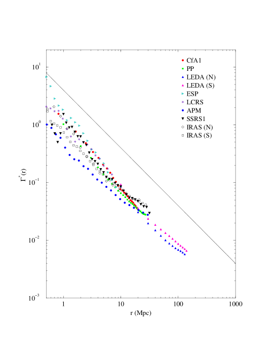
Figure 2: The spatial density $\Gamma(r)$ computed in some VL samples of CfA1, PP, LEDA, APM, ESP, LCRS, SSRS1, IRAS and ESP (Sylos Labini et al., 1997).

Finally it must be noted that Dr. Guzzo based a part of his arguments on the fact that a luminosity bias is responsible of the shift of $r_{0}$ with sample size (see also [5] [4]). We do not enter into a detailed explanation of the inconsistencies of the usual argument about luminosity segregation [5] [16] [2] and we refer to [28] for a more detailed analysis. However we would like to remark that the authors (e.g. [16] [2]) who have addressed this concept have never presented any quantitative argument that explains the shift of $r_{0}$ with sample size. In this respect, an exception is represented by the paper of Davis et al.(1988) in which the authors claim that $r_{0}$ behaves as $R_{s}^{0.5}$. However for what concerns luminosity segregation, the meaningful parameter must be the absolute magnitude limit of the volume limited (VL) sample considered rather than the depth ($R_{s}$). Having fixed the limiting apparent magnitude of the catalog, at each $R_{s}$ would correspond a well defined absolute magnitude. The brightest galaxies are present yet in samples like CfA1, and hence according to the luminosity segregation paradigm, there is no reason one should expect that in deeper sample (like CfA2 or SSRS2) $r_{0}$ is increased. However this is actually the case [2] [16].

We have discussed in detail in [24] that the observation that the giant galaxies are more clustered than the dwarf ones, i.e. that the massive elliptical galaxies lie in the peaks of the density field, is a consequence of the self-similar behavior of the whole matter distribution. The increasing of the correlation length of the $\xi(r)$ has nothing to do with this effect, rather it is related to the sample size.

A last point requires a further clarification. Dr. Guzzo claims that $\Gamma(r)$ is a power law with $D\sim 1.2$ up to $r\sim 3.5h^{-1}Mpc$, then it shows a different scaling between $\sim 3h^{-1}Mpc$ and $30h^{-1}Mpc$ with fractal dimension $D\approx 2$ [9]. In our view there is a subtle point in this discussion that has not been previously appreciated.

Suppose now, for simplicity, we have a spherical sample of volume $V$ in which there are $N$ points, and we want to measure the conditional density. It is possible to compute the average distance between neighbor galaxies $\langle\Lambda\rangle$, in a fractal distribution with dimension $D$, and the result is

$$\langle\Lambda\rangle=\left(\frac{1}{A}\right)^{\frac{1}{D}}\Gamma\left(1+\frac{1}{D}\right)$$ (3)

where $\Gamma$ is the Euler’s gamma-function [30]. (Note that the prefactor $A$ is dependent on the luminosity selection function of the VL chosen). Clearly this quantity is related to the lower cut-off of the distribution $A$ (eq.1) and to the fractal dimension $D$. If we measure the conditional density at distances $r\mathrel{\hbox to0.0pt{\lower 3.0pt\hbox{$\mathchar 536\relax$}\hss}\raise 2.0pt\hbox{$\mathchar 316\relax$}}\langle\Lambda\rangle$, we are affected by a finite size effect. In fact, due the depletion of points at these distances we underestimate the real conditional density finding an higher value for the correlation exponent (and hence a lower value for the fractal dimension). In the limiting case at the distances $r\ll\langle\Lambda\rangle$, we can find almost no points and the slope is $\gamma=-3$ ($D=0$). In general, when one measures $\Gamma(r)$ at distances which correspond to a fraction of $\langle\Lambda\rangle$, one finds systematically an higher value of the conditional density exponent. Such a trend is completely spurious and due to the depletion of points at such distances. It is worth to notice that this effect gives rise to a curved behavior of $\Gamma^{*}(r)$ (the integral of $\Gamma(r)$ see [3] [28]) at small distances, because of its integral nature. This is exactly the case of the deepest VL of Perseus-Pisces which Guzzo et al.(1991) considered in their analysis, and for which $\langle\Lambda\rangle\sim 8h^{-1}Mpc$. A clarifying test in this respect would be to check whether this change of slope is actually present also in the others VL samples of the same survey, which have a larger number of points (and hence a lower $\langle\Lambda\rangle$). This test has been performed by [28] and the conclusion is that the change of slope is due a finite size effect rather being an intrinsic property of galaxy distribution.

Finally we would like to point out another point that is inconsistent in the arguments of Dr. Guzzo. He and his collaborators [9] found that $\Gamma(r)$ flattens at $\mathrel{\hbox to0.0pt{\lower 3.0pt\hbox{$\mathchar 536\relax$}\hss}\raise 2.0pt\hbox{$\mathchar 318\relax$}}30h^{-1}Mpc$. Up to this distance $r_{0}$ must be a linear fraction of $R_{s}$ in view of eq.2 and does not depend to any luminosity bias ! In our opinion [26] [28], this flattening is due to an incorrect treatment of the boundary conditions (see point 1). However if this behavior is real, Dr. Guzzo should conclude that galaxy distribution is homogeneous at $\sim 30h^{-1}Mpc$ and not at $\sim 100\div 200h^{-1}Mpc$ as he claims.

We conclude this discussion pointing out another element: the analysis of LEDA. Dr. Guzzo claims that the results coming from LEDA [6] [1] are “as having no meaning whatsoever”. In our opinion such a strong conclusion must be supported by quantitative arguments. We have done several tests on the LEDA database [6] [1] [28] and we have concluded that, although this sample is highly incomplete, the statistical results obtained are rather stable and robust. We refer to the previously mentioned papers for a more specific discussion.

4 Galaxy distribution at scale $r\geq 100\div 200h^{-1}Mpc$

We discuss now the behavior of the radial density in general, and then we consider the two cases of PP and ESP (see [25] [13] and [28] for a more detailed discussion on this point).

We focus on the possibility of extending the sample effective depth $R_{s}$. In order to discuss this question, it is important to analyze the properties of the small scale fluctuations. To this aim, we introduce the conditional density in the volume $V(r)$ (that can be a portion of a sphere) as observed from the origin, defined as

$$\Gamma_{i}^{VL}(r)=\frac{N_{i}^{VL}(<r)}{V(r)}=\frac{3Ap}{4\pi}r^{D-3}\;.$$ (4)

where the factor $p$ comes from the fact that a VL sample contains only a fraction $N_{i}^{VL}(R)=p\cdot N(<R)$ (where $p<1$) of the total number $N(<R)$ of galaxies in $V(R)$. If $\phi(L)dL$ is the fraction of galaxies whose absolute luminosity ($L$) is between $L$ and $L+dL$, $p$ is given:

$$0<p=\frac{\int_{L_{VL}}^{\infty}\phi(L)dL}{\int^{\infty}_{L_{min}}\phi(L)dL}<1$$ (5)

In Eq.5 $L_{VL}$ is the minimal absolute luminosity that characterizes the VL sample and $L_{min}$ is the fainter absolute luminosity (or magnitude $M_{min}$) surveyed in the catalog (usually $M_{min}\sim-11$). Computing $\Gamma_{i}(r)$, we expect (Fig.3) not to see any galaxy up to a certain distance $\langle\Lambda\rangle$. For distances somewhat larger than $\langle\Lambda\rangle$, we expect therefore a raise of the conditional density because we are beginning to count some galaxies and $\Gamma_{i}(r)$ is affected by the fluctuations due to the low statistics.

It is therefore important to be able to estimate and control the minimal statistical length $\lambda$, which separates the fluctuations due to the low statistics from the genuine behavior of the distribution. A simple argument for the determination on the length $\lambda$ is the following [25] [13] [28]. At small scale, where there is a small number of galaxies, there is an additional term, due to shot noise, superimposed to the power law behavior of $\Gamma_{i}(r)$, that destroys the genuine correlations of the system.( As we have discussed in [28] there should be considered also an intrinsic oscillating term for non-averaged out quantities: however for sake of clarity we avoid this discussion here.) Such a fluctuating term can be erased out by making an average over all the points in the survey. On the contrary, in the observation from one point, when the number of galaxies is large enough the shot noise becomes negligible. Roughly, this happens when the number of points is lager than $\sim 30$ (see Fig.3).

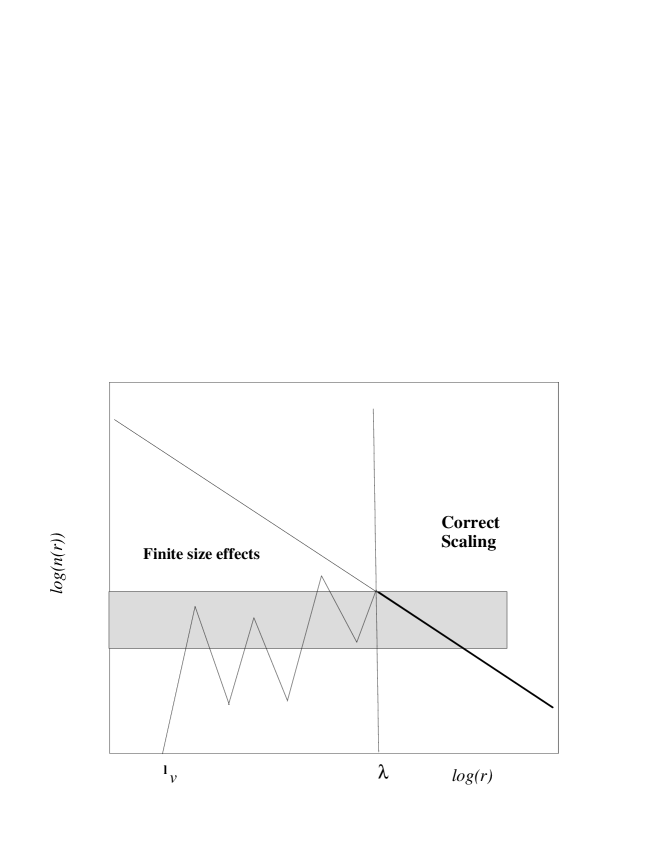
Figure 3: Behavior of the density computed from one point, in the case of a fractal distribution. At small distances below the average mean separation between neighbor galaxies, one finds no galaxies. Then the number of galaxies starts to grow, but this regime is strongly affected by finite size fluctuations. Finally the correct scaling region $r\approx\lambda$ is reached. In the intermediate region the density can be approximated roughly by a constant value. This leads to an apparent exponent $D\approx 3$ for the integrated counts. This exponent is not real but just due to the size effects.

This condition gives (from Eq.4)

$$\lambda=5\left(\frac{4\pi}{Ap\Omega}\right)^{\frac{1}{D}}\approx\frac{20\div 60h^{-1}Mpc}{\Omega^{\frac{1}{D}}}.$$ (6)

for a typical VL sample with $M_{VL}\approx M^{*}$, where $A$ corresponds to the amplitude of the conditional density of all galaxies [25] [28]. This can be estimated from the amplitude of $\Gamma(r)$ in a VL sample divided by the correspondent $p$ as defined in Eq.5. We find (for typical catalogues) $B\approx 10\div 15(h^{-1}Mpc)^{-D}$ [25]. The corresponding value of $\lambda$ are reported in Tab.2.

Survey	$\Omega(sr)$	$\lambda(h^{-1}Mpc)$
CfA1	1.8	15
CfA2 (North)	1.3	20
SSRS1	1.75	15
SSRS2	1.13	20
PP	1	40
LEDA	2 $\pi$	10
IRAS	2 $\pi$	15
ESP	0.006	300

Table 2: The minimal statistical length $\lambda$ for several redshift surveys.

The difference between $\Gamma(r)$ and $\Gamma_{i}(r)$ is straightforward: the latter quantity is not an average one. However it is an integrated one. The differential density is shells is clearly much more noisy, because it is not averaged neither integrated. We have computed the $\Gamma_{i}(r)$ in the various VL samples of Perseus-Pisces redshift survey, and we show the results in Fig.4. In the less deeper VL samples (VL70, VL90) the smooth behavior of the density is weakly defined because in this case the finite size effects are very important as the distances involved are $r<\lambda$ (Eq.6). We note that about the same scales we find a very well defined power law behavior by the correlation function analysis. In the deeper VL samples (VL110, VL130) a smooth and well defined behavior is reached for distances larger than the scaling distance ($\Omega=0.9\,sr$) $r\approx\lambda\sim 50h^{-1}Mpc$. The fractal dimension is $D\approx 2$ as the one measured by the average conditional density.

Figure 4: The spatial density $\Gamma_{i}(r)$ computed in the VL sample cut at $70,90,110,130h^{-1}Mpc$ . In the case of VL70 and VL90 the density is dominated by large fluctuations and it has not reached the scaling regime. In the samples VL110 and VL130 the density is dominated by large fluctuations only at small distances, while at larger distances, after the Perseus Pisces chain at $50h^{-1}Mpc$, a very well defined power law behavior is shown, with the same exponent of the correlation function (i.e. $D=2$)

For relatively small volumes it is possible to recover the correct scaling behavior for scales of order of $\langle\Lambda\rangle$ (instead of $\sim 10\langle\Lambda\rangle$) by averaging over several samples or, as it happens in real cases, over several points of the same sample when this is possible. Indeed, when we compute the correlation function, we perform an average over all the points of the system even if the VL sample is not deep enough to satisfy the condition expressed by Eq.6.

Now, if we look at the density in shells, this will be dominated by fluctuations, as it is not a cumulative distribution. Note that if the distribution would became homogenous, as Guzzo et al.[9] found, at $\sim 30h^{-1}Mpc$, then at 3 times the homogeneity scale the distribution would present a rather regular behavior. This is clearly not the case.

Let us now briefly discuss the properties of the ESP catalog. As the redshifts involved are quite large a particular care is devoted to the construction of the VL subsamples for the case of ESP. We have used various distance-redshift ($d(z)$) and magnitude-redshift ($m(z)$) relations. Moreover the data are selected in the blue-green and even if the redshifts of galaxies are moderate ($z\leq 0.2$), K-corrections are needed to compute the absolute magnitude of galaxies. The corresponding magnitude-redshift relation is

$$m-M=25+5\log_{10}\left(d(z,q_{0})(1+z)\right)+a(T)z$$ (7)

where we have used the functional forms of the K-correction $a(T)z$ as a function of redshift. $a(T)$ depends on the morphological type $T$ and goes from $a\sim 2$ for the Scd galaxies to $a\sim 3.7$ for the E/S0 galaxies. It is not possible to apply the K-correction to each morphological type because over the $\>17^{th}$ magnitude it is not possible to recognize the Hubble type from visual inspection. To overcame this problem we have adopted a statistical approach: we have assumed various percentage of late and early-type galaxies. The observed percentage in nearer samples is $\>70\%$ of late and $\>30\%$ of early type galaxies. We have performed a number of tests by varying these percentages to show that the final result depends weakly on the adopted values. We note that varying these percentages change the number of points in the VL subsamples as the absolute magnitude can change of about a unit.

The behavior of the number-distance relation in the standard FRW model depends strongly on the value of the deceleration parameter $\>q_{0}$ for high redshift $\>z>0.5$, while for $\>z<0.2$ the relativistic corrections are very small for all reasonable $\>q_{0}$.

All the samples show a highly fluctuating behavior for the space density as it is reported by Dr. Guzzo. It is very difficult in this case to identify a clear power law behavior. However we stress that an homogeneous distribution (say at $50h^{-1}Mpc$) would show a very smooth and flat behavior for $\Gamma_{i}(r)$ at these distance scales. This is clearly not the case.

It is very interesting, in our opinion, to study also the case of a purely Euclidean space. In this case we can write the $d(z)$ relation simply as:

$$d=\frac{c}{H_{0}}z$$ (8)

and the $m(z)$ relation (without K-corrections):

$$m-M=5\log_{10}\left(d(z)\right)+25\;.$$ (9)

In this case the volume grows as $\sim z^{3}\sim d^{3}$. The behavior of the radial density in the Euclidean case is reported in Fig.5.

Figure 5: The spatial density $\Gamma_{i}(r)$ computed in a VL samples of ESP. A the power law behavior with $D\approx 2$ is shown for $r\mathrel{\hbox to0.0pt{\lower 3.0pt\hbox{$\mathchar 536\relax$}\hss}\raise 2.0pt\hbox{$\mathchar 318\relax$}}300h^{-1}Mpc\approx\lambda$, even though with strong fluctuations

From this figure it is possible to see the effect of the finite size fluctuations: the scaling region begins at $\lambda\sim 300\div 320h^{-1}Mpc$ for all the VL subsamples. For smaller distances the statistical fluctuations dominate the behavior of $\Gamma_{i}(r)$. It seems that in this case the power law behavior for $r\mathrel{\hbox to0.0pt{\lower 3.0pt\hbox{$\mathchar 536\relax$}\hss}\raise 2.0pt\hbox{$\mathchar 318\relax$}}\lambda\approx 320h^{-1}Mpc$ is better defined than in the previous case. The fractal dimension turns out to be $D\approx 2.2$.

The K-correction, that must be applied for the Hubble shift of the galaxy spectra, can change the absolute magnitude of a unit. This correction is due to a systematic effect for each morphological type. As we put these correction in a random way we are mixing a systematic effect with a random correction. In this way we can only check the stability of the results but we cannot hope to obtain a better fit [28] By doing this [28] we find a marginal power law decaying of the conditional density. Therefore we may conclude that there is a weak evidence that the fractal dimension is $\>D\approx 2$ in this sample due to the poor statistics.

There are several other evidences in our opinion that point towards a fractal distribution of galaxies at very large scale, and in particular they are the density behavior from one point in the LCRS and the behavior of the galaxy numbers counts as a function of the apparent magnitude [28]. However we stress again that, due to the lackness of complete redshift measurements, these evidences are statistically weaker than the ones up to one hundred Megaparsec.

5 Discussion and Conclusions

Only after clarification of the small scale galaxy correlations it is possible to investigate the large scale ones. For what concerns the meaning of the so-called “correlation lengths” of galaxies and clusters, the behavior of the conditional density up to $\sim 100h^{-1}Mpc$ is enough to give us the elements for a revision of both the statistical methods usually used in the data analysis as well as the theoretical approach (i.e. linear non-linear dynamics, etc.). We refer the interested reader to [28] for a more complete discussion of the implications of the existence of a fractal distribution of matter, at least, up to $\ 100h^{-1}Mpc$.

Table 3: The volume limited samples of various catalogs (not still published and analyzed) are characterized by the following parameters: - $R_{VL}(h^{-1}Mpc)$ is the depth of the VL sample considered with absolute magnitude limit $M_{VL}$ - $\Omega$ is the solid angle - $R_{s}(h^{-1}Mpc)$ is the radius of the largest sphere that can be contained in the catalog volume. This gives the limit of statistical validity of the sample. - $r_{0}(h^{-1}Mpc)$ is the length at which $\xi(r)\equiv 1$. (distance are expressed in $h^{-1}Mpc$).

Sample	$\Omega$ ($sr$)	$R_{VL}$	$M_{VL}$	$R_{s}$	$r_{0}$
CfA2	1.83	101	-19.5	22	7
CfA2	1.83	160	-20.5	36	12
SLOAN	$\pi$	400	-19	185	60
SLOAN	$\pi$	600	-20	275	90
2dF (South)	0.28	550	-19	50	15
2dF (South)	0.28	870	-20	100	30

Let us now remark the predictions for future galaxy redshift surveys. According to the standard interpretation, the length $r_{0}\simeq 5h^{-1}Mpc$ characterizes the physical properties of galaxy distributions. Therefore deeper samples like CfA2 and SLOAN should simply reduce the error bar, which is now considered to be about $10\%$. A possible variation of $r_{0}$ with absolute magnitude, due to a luminosity bias, is considered plausible but it has never been quantified. This should be checked by varying independently absolute magnitude and depth of the volume limited samples. However, from this interpretation, the value of $r_{0}=5h^{-1}Mpc$, corresponding to a volume limited of CfA1 with $M=-19.5$, should not change when considering in CfA2 and SLOAN volume limited samples with the same solid angle $\Omega$ and the same absolute magnitude limit ($M=-19.5$).

In our interpretation, instead, $r_{0}$ is spurious, and it scales linearly with the radius $R_{s}$ of the largest sphere fully contained in the volume limited samples. Therefore we predict for the volume limited sample of CfA2 with $M=-19.5$ (with a solid angle of $\Omega=1.1\;sr$ [16]) $r_{0}\approx 7h^{-1}Mpc$ (if, in the final version of the survey the solid angle is $\Omega=1.8$, the value of $R_{s}$ increases accordingly, and the value of $r_{0}$ is shifted up to $\sim 9h^{-1}Mpc$). Note however that for the deepest volume limited CfA2 sample ($M\mathrel{\hbox to0.0pt{\lower 3.0pt\hbox{$\mathchar 536\relax$}\hss}\raise 2.0pt\hbox{$\mathchar 316\relax$}}-20$) we predict instead $r_{0}\approx 15\div 20h^{-1}Mpc$. For the volume limited sample of the full SLOAN with $M=-19.5$ ($\Omega=\pi$), our prediction is that $r_{0}\approx 65h^{-1}Mpc$. It is clear that however, the first SLOAN slice gives smaller values because the solid angle is be small. In Tab.3 we report the predictions for $r_{0}$ in the next future surveys.

Finally we would like remark that if it is true that the fractal analysis, as good wine, must be taken with “moderation”, it is also true that up to now the usual approach in this field has suffered of abstinence. We hope that the present discussion will evolve in a more constructive and cooperative way between the field of statistical mechanics and large scale structure astrophysics, hoping to drink together some good wine.

References

- [1] Amendola L., Di Nella H., Montuori M. and Sylos Labini F. 1997, Fractals, in print astro-ph/9711148
- [2] Benoist C., 1996 et al.Astrophys. J. 472, 452
- [3] Coleman, P.H. & Pietronero, L., 1992 Phys.Rep. 231, 311
- [4] Davis, M., in the Proc of the Conference ”Critical Dialogues in Cosmology” N. Turok Ed. (1997) World Scientific
- [5] Davis M. et al., 1988 Astrophys. J. Lett. 333 L9
- [6] Di Nella H., et al.1996 Astron. Astrophys. Lett 308, L33
- [7] Durrer R., Eckmann J.-P., Sylos Labini F., Montuori M., Pietronero L. 1997 Europhys. Lett. 40, 491
- [8] Guzzo L., 1997 New Astronomy 2, 517
- [9] Guzzo L. et al., 1991 Astrophys. J. Lett., 382 L5
- [10] Loveday J. et al., 1995 Astrophys. J. 442, 457
- [11] Mandelbrot B.B., 1982 The Fractal Geometry of Nature, Freeman, New York
- [12] Mandelbrot B.B., 1998 in the Proc. of the Erice School ”Astrofundamental physics” Eds. N. Sanchez and H. de Vega
- [13] Montuori M., Sylos Labini F. Gabrielli A., Amici A. and Pietronero L. 1997 Europhys Lett. 31, 103
- [14] Montuori M. and Sylos Labini F. 1997 Astrophys. J. Lett. 487, L21
- [15] Montuori M., Sylos Labini F. and Amici A. 1997 Physica A. 246, 1
- [16] Park C., Vogegely M. and Geller M. 1994 Astrophys. J. 431, 569
- [17] Peebles P. J. E., 1980 The Large scale structure of the universe, Princeton Univ. Press
- [18] Peebles P. J. E., 1993 Principles of physical Cosmology, Princeton Univ. Press
- [19] Pfenniger D. and Sylos Labini F.,1998 In preparation
- [20] Pietronero, L. 1987 Physica A, 144, 257
- [21] Pietronero, L., Montuori, M. and Sylos Labini, F., 1997 p.24-49 in the Proc of the Conference ”Critical Dialogues in Cosmology” N. Turok Ed. World Scientific
- [22] Provenzale A., Guzzo L. and Murante G. 1994, MNARS, 266, 555
- [23] Sylos Labini F., 1994 Astrophys. J., 433, 464
- [24] Sylos Labini F., Pietronero L., 1996 Astrophys. J. 469,28
- [25] Sylos Labini F., Gabrielli A., Montuori M. and Pietronero L., Pietronero L., 1996a Physica A 266, 195
- [26] Sylos Labini F., Montuori M. and Pietronero L., 1996b Physica A 230, 336
- [27] Sylos Labini F., Amendola L., 1996 Astrophys. J. Lett. 468 L1
- [28] Sylos Labini F., Montuori M., Pietronero L., 1998 Phys.Rep. 291 In print.(astro-ph/9711073)
- [29] Sylos Labini F., Montuori M., 1998 Astron. Astrophys In print (astro-ph/9711134)
- [30] Sylos Labini F., Gabrielli A., Montuori M. and Pellegrini S. (1998) preprint