Abstract

I give a status report and outlook concerning the use of the cosmic microwave background anisotropies to constrain the inflationary cosmology, and stress its crucial role as an underlying paradigm for the estimation of cosmological parameters.

SUSSEX-AST 98/1-1
astro-ph/9801148

1 Introduction

For a long time now, inflation has been the leading paradigm for the origin of cosmological structures. This is largely due to its continuing success in confrontation with a wide range of observations, but also due in part to its theoretical simplicity compared to rivals such as cosmic strings, both in terms of making predictions for the perturbations and in the form (gaussian and adiabatic) of perturbations generated.

The interaction between observations and theoretical modelling of inflation plays a two-fold role in cosmology. The most-emphasized role is the possible use of observations, especially of cosmic microwave background anisotropies, to support or rule out the inflationary paradigm as the source of structures (see Liddle & Lyth 1993 for a review). Such a program may well offer the first glimpses of possible physics at very high energies. Much less has been said about the second role of inflation — that in providing a simple framework for structure formation, it is crucial in enabling the high-accuracy determination of more mundane cosmological parameters such as the Hubble constant and the density parameter. I shall focus particularly on this aspect towards the end of this review.

2 Inflation

Inflation is defined as any epoch of the Universe’s history during which the scale factor $a(t)$ is accelerating. In fact, we have yet to prove conclusively that this is not happening at the present epoch, but here I am interested in whether such a behaviour might have happened in the Universe’s distant past. I actually prefer to use the Hubble parameter $H=\dot{a}/a$ to write this in a somewhat different way

$$\ddot{a}>0\quad\Longleftrightarrow\quad\frac{d}{dt}\left(\frac{H^{-1}}{a}\right)<0\,,$$ (1)

where dots are of course time derivatives. The quantity $H^{-1}$ is the Hubble length, the principal characteristic scale of an expanding Universe, and dividing it by $a$ switches to comoving coordinates, i.e. the behaviour of relative to the expansion. In words, inflation is precisely the condition that the comoving Hubble length is decreasing with time. Since in comoving units all the objects just remain where they are as the Universe expands, and since at any epoch the Hubble length is a good estimate of how far light can travel during that epoch, this is telling us that inflation acts like a zoom lens, focussing in on an ever-tinier part of the initial region. That’s why, for example, inflation can solve the flatness problem; even if curvature is important initially, when we zoom in on a tiny region the curvature becomes negligible, and enough ‘zooming’ can more than compensate for the subsequent increase of the comoving Hubble length after inflation ends.

Inflation’s ability to generate large-scale perturbations is all down to the behaviour of the Hubble length, because it means that a given length scale may start well inside the Hubble radius, but finish up well outside it. Any irregularities existing at that time become ‘frozen-in’, unable to evolve. If we lived in a purely classical world, this would lead to a perfectly homogeneous Universe, simply because the assumption that the initial energy density be finite requires that there cannot be irregularities down to arbitrarily small scales.

Fortunately, we live not in a classical Universe but a quantum one, and the uncertainty principle implacably opposes inflation’s attempts to make a perfectly smooth Universe. More so, it does this in a manner which is readily predictable for a given inflationary model. It turns out that quantum fluctuations give rise to two types of perturbations in the Universe, density perturbations and gravitational waves. These both take on a classical character once they are on scales well in excess of the Hubble length.

In order to give definite predictions for these, it is necessary to have a definite model for the inflationary expansion rather than just the hand-waving sketch I’ve given above. Here I want to stress that inflationary model-building has become quite a complicated and sophisticated occupation, and in presentations like this one necessarily gives an oversimplified picture. Bear that in mind, and I’ll also remind you of it later.

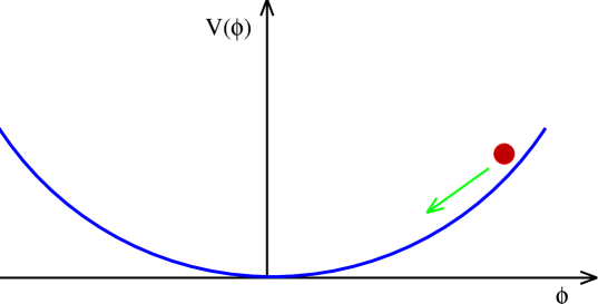
Figure 1: A schematic scalar field potential.

The acceleration equation

$$\frac{\ddot{a}}{a}=-\frac{4\pi G}{3}\left(\rho+3p\right)\,,$$ (2)

immediately tells us that we’re going to need something a little out of the ordinary, namely $p<-\rho/3$. The standard way of achieving this uses a scalar field, the sort of thing which crops up all over the place in modern particle physics theories, especially when symmetry breaking is under consideration. The standard simplified picture, which does in fact cover a large fraction of the currently popular models, is that there is only one scalar field, and that it evolves classically by slow-rolling down a self-interaction potential $V(\phi)$ such as that shown in Figure 1. Either of these assumptions can be altered, giving more complicated models, but the bulk of my discussion will stay with the simplest case.

Such a homogeneous scalar field has effective energy density and pressure

$$\rho_{\phi}=\frac{1}{2}\dot{\phi}^{2}+V(\phi)\quad;\quad p_{\phi}=\frac{1}{2}\dot{\phi}^{2}-V(\phi)\,,$$ (3)

and so the condition for inflation is satisfied as long as the potential dominates over the kinetic term. This will clearly happen if the potential is sufficiently flat; in fact, the flatness condition is very weak and so inflation is quite generic.

In principle, $V(\phi)$ is predictable from fundamental theories of physics. In practice there is as yet no clear guidance, and instead we treat it as a free function to be constrained by observations.

3 Describing the perturbations

If the inflationary expansion is rapid enough, physical conditions during inflation will change little between the origin of perturbations on the largest interesting scales and the smallest, so as a rough rule of thumb we expect that the perturbations will be nearly scale-invariant. For a long time, the perturbations were indeed taken to have that form. However, more recently the observations have reached such quality that the scale-invariance approximation is no longer an adequate description, and we have to do better. This is in no way a set-back (or climb-down) for inflation — it is an impressive success that the theory has done so well that we now regard small corrections to the initial picture as significant and observationally testable.

The breaking of scale-invariance will depend on the form of the potential $V(\phi)$ (it being the only input information), so we quantify this by defining two slow-roll parameters (Liddle & Lyth 1992)

$$\epsilon\equiv\frac{m_{{\rm Pl}}^{2}}{16\pi}\left(\frac{V^{\prime}}{V}\right)^{2}\quad;\quad\eta\equiv\frac{m_{{\rm Pl}}^{2}}{8\pi}\frac{V^{\prime\prime}}{V}\,,$$ (4)

where prime means a derivative wrt $\phi$, and $m_{{\rm Pl}}=G^{-1/2}$ is the Planck mass. Inflation requires that both these be less than one, in order to maintain dominance of the potential. The first measures the slope of the potential, the second its curvature.

The terminology I will use isn’t very important; density perturbations are specified by $\delta_{{\rm H}}(k)$ and gravitational waves by $A_{{\rm G}}(k)$ where $k$ is the comoving wavenumber. For scale-invariant spectra these are both independent of $k$; the power spectrum $P(k)\propto k\delta_{{\rm H}}^{2}$. Under the inflationary paradigm, these spectra are responsible for all the observed structures, with gravitational waves at best only significantly influencing large-angle microwave background anisotropies.

The formulation I’ll describe is based on a perturbative approach, where we expand the (log of the) spectra in terms of log(wavenumber) about some scale $k_{*}$:

$$\ln\delta_{{\rm H}}^{2}(k)=\ln\delta_{{\rm H}}^{2}(k_{*})+(n_{*}-1)\ln\frac{k}{k_{*}}+\frac{1}{2}\left.\frac{dn}{d\ln k}\right|_{*}\,\ln^{2}\frac{k}{k_{*}}+\cdots\,,$$ (5)

and truncate at some level. For example

First term: Harrison–Zel’dovich spectrum (constant $\delta_{{\rm H}}$).

Second term: Power-law spectrum with spectral index $n$.

Third term: Includes scale-dependence of the spectral index.

Current observations require at least the second term and normally people stop there. I’ll return to the third one later. The second term gives the power-law approximation, and the observables can be very nicely computed in terms of the slow-roll parameters (Liddle & Lyth 1992):

$$n=1-6\epsilon+2\eta\quad;\quad n_{{\rm G}}=-2\epsilon\quad;\quad\frac{A_{{\rm G}}^{2}(k_{*})}{\delta_{{\rm H}}^{2}(k_{*})}=\epsilon=-\frac{n_{{\rm G}}}{2}\,.$$ (6)

If slow-roll holds very well ($\epsilon\ll 1$, $|\eta|\ll 1$) we get scale-invariant density perturbations and negligible gravitational waves. Note also that although $\epsilon$ is positive by definition (the field always rolls downhill), $\eta$ can have either sign and $n$ can be greater or smaller than one. The final relation, giving the ratio of the spectra in terms of $n_{{\rm G}}$, is known as the consistency relation; it represents the inevitable ‘entanglement’ of the density perturbations and gravitational waves due to their common origin in the single function $V(\phi)$. In the unlikely event of it proving testable, it represents a very distinctive prediction of inflation.

4 COBE

The COBE observations have a very simple interpretation in terms of inflation. Because the COBE beam is so wide, it only probes scales larger than the horizon at the time of decoupling, so perturbations have not had time to evolve and are captured in their primordial form. In particular, the observed anisotropies do not depend on cosmological parameters such as the hubble constant $h$ and the baryon density $\Omega_{{\rm B}}$.

COBE determines the perturbation amplitude extremely well, to about 10% accuracy, but is unable to distinguish the effect of density perturbations and gravitational waves. Its most useful application is to normalize the density perturbation spectrum; Bunn et al. (1996) obtained the result

$$\delta_{{\rm H}}=1.91\times 10^{-5}\,\frac{\exp\left[1.01(1-n)\right]}{\sqrt{1+0.75r}}\,,$$ (7)

using techniques described by Bunn & White (1995, 1997). Here $\delta_{{\rm H}}$ is the perturbation amplitude at the present Hubble radius, and $r=12.4A_{{\rm G}}^{2}/\delta_{{\rm H}}^{2}$ approximately measures the relative importance of gravitational waves and density perturbations in generating the anisotropies. The factor 12.4 comes from analytic evaluation assuming only the Sachs–Wolfe effect applies and perfect matter domination at last scattering; that the above expression contains the factor 0.75 indicates that this approximation fails at the tens of percent level on COBE scales.

COBE fixes the energy scale of inflation as (Bunn et al. 1996)

$$V_{*}^{1/4}=\left(6.6\times 10^{16}\,{\rm GeV}\right)\epsilon^{1/4}\quad\pm 5\%\,,$$ (8)

where $*$ indicates the value when the observed perturbations were generated. For a specific model $\epsilon$ is known and so this can be given exactly. Unless $\epsilon$ is tiny, which is perfectly possible in some models, the energy scale is around that expected of Grand Unification.

The spectral index $n$ is only very weakly constrained by COBE, due to the limited range of scales sampled.

Figure 2: A compilation of measurements of microwave background anisotropies, by Martin White. The detections (1-sigma errors) are COBE (3 open circles), Tenerife and BAM (filled squares), Python (2 stars), Saskatoon (5 filled triangles), ARGO (2 open squares), MAX (open triangle), CAT (2 filed circles) and OVRO (cross). The 95% confidence upper limits are SuZIE, ACTA and Ryle. For a detailed discussion see Anthony Lasenby’s contribution to these proceedings.

5 The current compilation

Nowadays, measured anisotropies go well beyond COBE, with a host of experiments reporting detections on a range of angular scales. Figure 2 shows a recent compilation by Martin White. The data are encouragingly compatible with inflationary preconceptions, but unfortunately at present don’t allow us to say much more; the predictions on smaller angular scales (larger $\ell$) depend on all the cosmological parameters and the observational errors are larger than one desires. The compilation does indicate a lower limit on $n$, which is somewhat model-dependent but is around $0.75$, and at the moment that is its main inflationary implication.

6 Solving cosmology …

The upcoming launch of the MAP and Planck satellites offers the prospect that cosmology could be more or less solved, in the sense that its most crucial parameters might be measured to a satisfyingly high accuracy (Jungman et al. 1996; Bond et al. 1997; Zaldarriaga et al. 1997). However, there are rather a lot of parameters which might come into play. Most attention has been focussed on the cosmological parameters, such as the Hubble constant $h$, total matter density $\Omega_{0}$, baryon density $\Omega_{{\rm B}}$, cosmological constant $\Omega_{\Lambda}$, hot dark matter density $\Omega_{{\rm hdm}}$ and the optical depth to the last-scattering surface $\tau_{{\rm c}}$. Some of these might be fixed by assumption, but as a very minimum $h$, $\Omega_{{\rm B}}$ and $\tau_{{\rm c}}$ must be determined observationally.

However, in this article I want to turn attention to the inflationary input. As I stressed at the beginning, this is absolutely crucial as a paradigm in cosmology. If we don’t know the initial perturbation spectra, we have no chance of interpreting observed microwave anisotropies in terms of the cosmological parameters. This is potentially a very serious problem, since without guidance the perturbations could be free functions which need not be simple.

Fortunately, most models of inflation give very simple predictions, and are summarized in only two or three parameters, namely $\delta_{{\rm H}}$, $n$ and perhaps $r$. However, scale-dependence of $n$ is possible, and in accordance with the Taylor expansion of Eq. (5) it can be incorporated by inclusion of derivatives $dn/d\ln k$, $d^{2}n/d\ln k^{2}$ and so on. These represent extra parameters which must be determined from observations.

If extra parameters are introduced, then the determination of all parameters will deteriorate. We have estimated the extent of this deterioration (Copeland et al. 1997) for a configuration of the Planck satellite including polarized detectors. It is shown in Table 1.

Table 1: Estimated parameter errors (one-sigma) for the Standard CDM model, as extra scale-dependence is introduced.

Parameter	Planck 140 GHz channel
	with polarization
$\delta\Omega_{{\rm b}}h^{2}/\Omega_{{\rm b}}h^{2}$	$0.007$	$0.009$	$0.01$
$\delta\Omega_{{\rm cdm}}h^{2}/h^{2}$	$0.02$	$0.02$	$0.02$
$\delta\Omega_{\Lambda}h^{2}/h^{2}$	$0.04$	$0.05$	$0.05$
$\delta\tau_{{\rm C}}$	$0.0006$	$0.0006$	$0.0006$
$\delta n$	$0.004$	$0.04$	$0.14$
$\delta r$	$0.04$	$0.05$	$0.05$
$dn/d\ln k$	$-$	$0.006$	$0.04$
$d^{2}n/d(\ln k)^{2}$	$-$	$-$	$0.005$

We see that permitting scale dependence of $n$ primarily only affects the determination of $n$, and not the other cosmological parameters, which is an encouraging conclusion. It suggests that if the modelling of inflation turns out to be over-simplified, the influence on parameter determination will not be too great. On the other hand, it is clear that $n$ cannot be measured as well as has been claimed (e.g. Bond et al. 1997; Zaldarriaga et al. 1997) unless it is assumed that the spectrum is a perfect power-law.

7 Inflationary complications

Now, as promised, I turn to the question of possible complications to the inflationary modelling. First of all, one can ask whether we are in a position to compute the perturbations at the 1% or so accuracy level demanded by MAP and Planck. Finally, the answer to this appears to be ‘yes’; the last problem (gravitational waves in open Universe models — see below) has been solved during the last year and there are no existing models in which the perturbations cannot be computed, at least through numerical integration of the relevant mode equations, to the required accuracy.

7.1 Single-field models

So far we’ve been sticking to models with a single scalar field, with $V(\phi)$ kept as a free function. Normally the slow-roll approximation gives a very accurate analytic result (Grivell & Liddle 1996). However, a sufficiently complicated potential may lead to a failure of slow-roll severe enough that the slow-roll approximation is not good enough (Wang et al. 1997), and the numerical results are required. However, we have found (Copeland et al. 1998) that this need not be a bad thing; in particular, the near-failure of slow-roll makes it far more likely that the scale-dependence of $n$ is observable, which allows one to determine more information about the inflaton potential than would otherwise have been available. Further, it would take a bizarre conspiracy for the slow-roll approximation to be failing, but yet for us to be oblivious to this. If things are going wrong to the extent that numerical computation is needed, we will know it.

The main worry in fact for the single-field models described so far is that many models [particularly those constructed under the currently-popular hybrid inflation strategy (see Lyth 1996 for a review)] predict a negligible level of gravitational waves. This limits seriously the amount of information that can be inferred about $V(\phi)$, which cannot even be determined uniquely if the gravitational waves cannot be detected.

7.2 Multi-field models?

It is certainly possible that more than one scalar field can be dynamically important, and this can lead to a range of new phenomena. The perturbations may have an isocurvature component as well as the usual adiabatic one, and may even be non-gaussian. The perturbations can still be computed accurately, but now only on a model-by-model basis rather than via an all-encompassing formalism like that I’ve demonstrated for single-field models. This makes it much harder to ‘guess’ viable models from the observations.

However, calculational complications aside, a specific model of this type is as easy to exclude using observations as a single-field model.

7.3 Open inflation models?

Open inflation models are an unfortunate late addition into the inflationary model zoo. Although dating back almost to the beginnings of inflation (Gott 1982), it is only relatively recently that they have been appreciated as a serious model. They rely on quantum tunnelling to generate an open Universe within an inflationary sea.

For a long time the perturbations in these models could not be computed (especially the gravitational waves), but finally the technology is in place (Sasaki et al. 1997; Bucher & Cohn 1997), and predictions can be obtained from them as readily as the more conventional models.

Mathematically they are much nastier models (for example the mode functions on hyperbolic geometry are very unpleasant indeed) than ones giving a flat spatial geometry. Fortunately, the spatial geometry is very readily measurable, even before the satellites go up, and hopefully these models will soon be consigned to the dustbin.

7.4 Inflation not correct?

If inflation is not in fact the correct theory for the origin of perturbations, this should be obvious from the observations. The inflationary prediction of passive, super-horizon perturbations is very distinctive, and leads to the familiar oscillations in the radiation angular power spectrum. If inflation is correct the observations should highly overdetermine the various parameters of the big-bang model, reassuring us that we are on the right track.

But here is a good point to stress once more the importance of inflation as a paradigm for the initial conditions. For example, it seems rather unlikely that predictions at the one percent level could come from the rival topological defect scenario in the forseable future, due to the horrendous non-linearities involved in the computations. Without accurate theoretical predictions for the anisotropies, huge extra uncertainties enter the cosmological parameter estimation game and severely dent one’s ability to measure any of them.

8 Conclusions

My main point of emphasis has been to stress that the inflationary paradigm is a crucial underpinning of attempts to measure cosmological parameters from the microwave background. It provides a framework in which accurate predictions can readily be made, enabling the maximum to be squeezed out of quality observations. We are fortunate indeed that not only is the model theoretically appealing, but that it also stands in excellent shape when confronted with present data. We can only hope that in ten years time, when the large zoo of inflation models have been confronted with the new observations, that things may still look so good.

References

Bond, J.R., Efstathiou, G. and Tegmark, M., 1997, Mon. Not. R. Astron. Soc. 291, L33

Bucher, M. and Cohn, J.D., 1997, Phys. Rev. D 55, 7461

Bunn, E.F., Liddle, A.R. and White, M., 1996, Phys. Rev. D 54, 5917R

Copeland, E.J., Grivell, I.J. and Liddle, A.R., 1997, Sussex preprint astro-ph/9712028

Copeland, E.J., Grivell, I.J., Kolb, E.W. and Liddle, A.R., 1998, Sussex preprint

Gott, J.R., 1982, Nature 295, 304

Grivell, I.J. and Liddle, A. R., 1996, Phys. Rev. D 54, 7191

Jungman, G., Kamionkowski, M., Kosowsky, A. and Spergel, D.N., 1996, Phys. Rev D 55, 7368

Liddle, A.R. and Lyth, D.H., 1992, Phys. Lett. B 291, 391

Liddle, A.R. and Lyth, D.H., 1993, Phys. Rep. 231, 1

Lyth, D.H., 1996, Lancaster preprint hep-ph/9609431

Sasaki, M., Tanaka, T and Yakushige, Y., 1997, Phys. Rev. D 56, 616

Wang, L., Mukhanov, V.F. and Steinhardt, P.J., 1997, Phys. Lett. B 414, 18

Zaldarriaga, M., Spergel, D. N. and Seljak, U., 1997, Astrophys. J. 488, 1