High Metallicity Mg II Absorbers in the $z<1$ Ly$\alpha$ Forest
of PKS 0454+039: Giant LSB Galaxies?

Abstract

We report the discovery of two iron–group enhanced high–metallicity Mgii absorbers in a search through 28 Ly$\alpha$ forest clouds along the PKS 0454+039 sight line. Based upon our survey and the measured redshift number densities of $W_{\rm r}({\hbox{{\rm Mg}\kern 1.00006pt{\sc ii}}})\leq 0.3$ Å absorbers and Ly$\alpha$ absorbers at $z\sim 1$, we suggest that roughly 5% of Ly$\alpha$ absorbers at $z\leq 1$ will exhibit “weak” Mgii absorption to a 5$\sigma$ $W_{\rm r}(\lambda 2796)$ detection limit of 0.02 Å. The two discovered absorbers, at redshifts $z=0.6248$ and $z=0.9315$, have $W_{\rm r}({\hbox{{\rm Ly}\kern 1.00006pt$\alpha$}})=0.33$ and 0.15 Å, respectively. Based upon photoionization modeling, the Hi column densities are inferred to be in the range $15.8\leq\log N({\hbox{{\rm H}\kern 1.00006pt{\sc i}}})\leq 16.8$ cm^-2. For the $z=0.6428$ absorber, if the abundance pattern is solar, then the cloud has $[\hbox{Fe/H}]>-1$; if its gas–phase abundance follows that of depleted clouds in our Galaxy, then $[\hbox{Fe/H}]>0$ is inferred. For the $z=0.9315$ absorber, the metallicity is $[\hbox{Fe/H}]>0$, whether the abundance pattern is solar or suffers depletion. Imaging and spectroscopic studies of the PKS 0454+039 field reveal no candidate luminous objects at these redshifts. We discuss the possibility that these Mgii absorbers may arise in the class of “giant” low surface brightness galaxies, which have $[\hbox{Fe/H}]\geq-1$, and even $[\hbox{Fe/H}]\geq 0$, in their extended disks. We tentatively suggest that a substantial fraction of these “weak” Mgii absorbers may select low surface brightness galaxies out to $z\sim 1$.

1 Introduction

Metal–line absorption in the intergalactic medium, or IGM, is astrophysically interesting because the absorption properties can be exploited to reveal the star formation, chemical enrichment, and ionization histories of the universe. This provides a motivation for studying metal lines in Ly$\alpha$ absorbers over as wide a redshift range as possible and for sampling transitions covering as many ionization levels and chemical species as possible (cf. Hellsten et al. (1997); Rauch, Heahnelt, & Steinmetz (1997)). Observations (Hu et al. (1995); Lu et al. (1996); Kim et al. (1997)) and numerical simulations (Miralda–Escudé et al. (1996); Zhang et al. (1997); Davé et al. (1997); Norman et al. (1997)) have revealed that the forest is rapidly evolving with redshift from $z\sim 4$ to $z\sim 1$, and that the absorbing gas is housed in a wide range of cosmic structures undergoing a wide range of dynamical processes. At $z\sim 2$, Ly$\alpha$ clouds contain the majority of the baryon content of the universe. At lower redshifts, Ly$\alpha$ clouds are thought to be more directly associated with low surface brightness and/or dwarf galaxies (Salpeter (1993); Shull et. al. (1996); Linder (1997)), with the outer disks and halos of high surface brightness galaxies (Lanzetta et al. (1995); Le Brun et al. (1996)), or with the remnant material left over from the formation of galaxies and/or small galaxy groups (van Gorkom et. al. (1996); Bowen, Blades, & Pettini (1996); Le Brun et al. (1996)). Studies of the metal content and ionization conditions in these low redshift forest clouds, especially in the context of their association (or lack of association) with galaxies, could provide the “missing–link” evidence necessary for inferring the evolving interplay between the IGM and galaxies or the presence of low surface brightness galaxies at higher redshifts.

A limited number of strong metal–line species have now been seen in high ionization transitions at $z\sim 2.5$ (Tytler et al. (1995); Cowie et al. (1995); Songaila & Cowie (1996)). However, the chemical and ionization conditions of Ly$\alpha$ clouds at low redshifts ($z\leq 1$) remain unexplored because they require time–intensive programs using HST. Relative to $z\sim 2.5$, the meta–galactic UV background flux (UVB) at $z<1$ is reduced by a factor of $\sim 5$ and its shape may be softened by stellar photons escaping bright field galaxies (Deharveng et al. (1997); Giallongo, Fontana, & Madau (1997); Bergeron et al. (1994), and references therein). Thus, the IGM ionization conditions may have evolved so that low ionization species, especially the resonant Mgii $\lambda\lambda 2976,2803$ doublet and several of the stronger Feii transitions, are detectable in Ly$\alpha$ clouds. As discussed below, these particular species are well suited for understanding chemical enrichment histories.

Songaila & Cowie (1996, hereafter SC96) detected Civ absorption in $\simeq 75$% of all Ly$\alpha$ clouds at $z\sim 2.5$ with $\log N({\hbox{{\rm H}\kern 1.00006pt{\sc i}}})\geq 14.5$ cm^-2 and concluded that roughly 50% of $\log N({\hbox{{\rm H}\kern 1.00006pt{\sc i}}})\leq 14.5$ cm^-2 clouds could have primordial abundances. They also reported Siiv and Cii absorption in a fraction of the Ly$\alpha$ clouds (including “partial” Lyman limit systems). Based upon the photoionization models of Bergeron & Stasińska (1986), SC96 find the metallicity of $z\sim 2.5$ Ly$\alpha$ clouds to be $[Z/Z_{\odot}]\sim-2$ and to be fairly uniform, with about 1 dex of scatter. They also report [Si/C] ratios consistent with Galactic Halo stars (metal poor late–type stars), in that the $\alpha$–group silicon is enhanced by a factor of three over the carbon. This conclusion, however, is sensitive to the assumed UVB continuum shape, especially the question of how much star bursting galaxies contribute to the UVB, and its non–uniformity, at higher redshifts (Giroux & Shull (1997)).

Considering the mechanisms and range of environments that could plausibly give rise to metals in what are traditionally known as Ly$\alpha$ clouds, it is difficult to understand a high level of uniformity in their chemical enrichment histories. As proposed by Tytler et al. (1995), there are at least three obvious mechanisms for the enrichment.

(1) The larger $N({\hbox{{\rm H}\kern 1.00006pt{\sc i}}})$ clouds may be gravitationally bound with internal gravitational instabilities in which they produce their own stars, which in turn distribute the metals throughout the cloud. This type of object has little distinction from a galaxy. This in situ process would likely give rise to a strong metallicity dependency with Hi column density, unless a well–tuned mechanism governing star formation yielded a uniform chemical enrichment history of the IGM, as suggested by Cowie et al. (1995). Such a mechanism would likely represent non–standard star formation processes.

(2) The metals may be produced in protogalaxies and then be widely distributed via mechanical ejection from merging events (Gnedin & Ostriker (1997)) or from correlated supernovae (SNe) (Cen & Ostriker (1992)). This implies that Ly$\alpha$ clouds formed after the metals were distributed around the metal producing galaxies. The scenario also predicts that the metal enriched Ly$\alpha$ clouds, as opposed to “Ly$\alpha$–only” clouds, would cluster like galaxies.

(3) Population III stars, formed at $z>10$ and somewhat uniformly spread throughout the IGM, may have distributed metals into the IGM prior to the first protogalaxies. A population of Ly$\alpha$ forest clouds that have been enriched by Population III stars may exhibit IGM chemical conditions that are relatively unchanged from the epoch of the first stars. If so, this population would be ideal for studying the intensity and continuum shape evolution of the UVB from $0<z<4$, since the changing ionization conditions could be used to deconvolve the non–evolving chemical conditions from the evolving UVB. As such, the detection of extremely metal poor stars in the Galaxy halo would also be very interesting, since their presence would suggest the presence of Population III stars (cf. Ostriker & Gnedin (1996)).

The chemical abundance pattern can serve as a clue to the origin, physical environment, and chemical enrichment history of any given Ly$\alpha$ absorber. There are at least two major uncertainties involved in measuring relative abundances using QSO absorption lines: ionization corrections and dust grain depletion patterns. The ionization correction provides good reason for observing a wide range of ionization levels. Moreover, the ionization corrections are sensitive to the intensity and continuum shape of the ionizing radiation, possibly providing even further leverage for understanding local environments and chemical enrichment history. Dust depletion does not effect all $\alpha$–group elements (for example, sulfur is not readily incorporated onto dust grains) nor all Fe–group elements (for example, zinc). However, those elements provide neither the strong UV absorption lines needed to accurately probe clouds with $\tau_{912}<1$, nor the transitions observable from the ground for redshifts below $z\sim 1$. The strongest observable transitions are the Mgii $\lambda\lambda 2976,2803$ doublet ($\alpha$–group), and Feii $\lambda 2344$, 2382, and 2600. Unfortunately, both magnesium and iron can deplete onto dust grains and their depletion levels are environment dependent.

For each of the three scenarios suggested above, it is expected that the relative elemental abundances of an enriched cloud should reflect the $\alpha$–group enhanced yield of Type II SNe (note that this is consistent with the results of SC96). In essence, the picture is simple: if the $\alpha$–group elements are enhanced relative to the Fe–group then the chemical enrichment has been dominated by Type II SNe. Based upon the [Si/Fe], [S/Fe], [O/Fe] ratios measured in Galactic halo stars, this pattern is seen for $\hbox{[Fe/H]}\leq-1$ (see Lauroesch et al. (1996)). In the case of scenario (3) presented above, it is likely that only a single burst, or episode, of star formation would have occurred and that the metal production arise exclusively from Type II SNe. In the case of scenario (2), the Ly$\alpha$ clouds would be far from the galaxies; the only metal enriched gas that could infiltrate clouds forming from the primordial IGM would necessarily be ejected from correlated Type II SNe bursts.

If the abundance pattern is more in line with solar proportions (i.e, $\hbox{[Mg/Fe]}\sim\hbox{[Si/Fe]}\sim\hbox{[Fe/H]}\sim 0$), then the picture is that Fe–group elements have been built up over a longer time scale via Type Ia SNe. This implies a star formation history local to the cloud that would have been relatively quiescent for $\sim\hbox{Gyr}$ prior to the epoch of the observed absorption. Thus, if a given Ly$\alpha$ cloud is measured to have $\hbox{[Fe/H]}\geq-1$ and [$\alpha$/Fe]–group abundance ratios near solar proportions, then one might infer that Type Ia SNe have played a role in the cloud’s chemical enrichment history. However, based upon uncertainties in Type II SNe yields, Gibson, Loewenstein, & Mushotzky (1997) have cautioned that the relative importance of Type Ia and Type II SNe as inter–cluster polluters remains uncertain.

A type of extended gas–rich object that is seen to have $\hbox{[Fe/H]}\geq-1$, and even $\hbox{[Fe/H]}\geq 0$, is the class of giant low surface brightness galaxies (Bothun, Impey, & McGaugh (1997); Pickering & Impey (1995); McGaugh (1994)). At low redshifts, the general population of low surface brightness galaxies are seen to outnumber high surface brightness galaxies by a factor of at least two (Dalcanton et al. (1997)). As such, these galaxies are important tracers of low density dark matter halos and structure formation from small over–density fluctuations. They also may represent environments where the pathways of star formation and chemical evolution reflect non–standard astrophysical processes (Bothun et al. 1997). If these objects are observable in absorption over a wide range of redshifts, they likely will provide us a unique astrophysical laboratory for broadening our present perspective on star and galaxy formation.

In this paper, we report the search for and discovery of Feii and Mgii doublet absorption in the Ly$\alpha$ forest along PKS 0454+039 sight line. In §2, we describe the data and analysis. In §3, we describe the sample of Ly$\alpha$ lines and our search method. The absorption properties of the detected systems are presented in §4. We apply photoionization models to the detected metal–line systems in §5, and briefly discuss the model results in §6. The implications of the results are addressed in §7. A brief summary is provided in §8.

2 Observations and Data Analysis

The Mgii and Feii transitions were searched for in an $R=45,000$ optical HIRES (Vogt et al. (1994)) spectrum. The Ly$\alpha$ line list was obtained from the $R=1300$ G190H and G270H FOS/HST spectra of Boissé et al. (1997, hereafter BBLD). Three images of the PKS 0454+039 field have been incorporated into our study so that we may attempt to identify the luminous objects giving rise to the absorption. Two are high–spatial resolution WFPC2/HST images using the F450W and F702W filters (Le Brun et al. 1997, hereafter LBBD). The third is the deep $R[6930/1500]$ image (centered on $\lambda 6930$ with a FWHM band pass of 1500 Å) taken from Steidel et al. (1995). We also draw upon the published (Steidel et al. (1995)) and unpublished (C. Steidel, private communication ) spectroscopic redshift measurements of the many objects along the line of sight to the QSO.

The HIRES spectrum was obtained and reduced as described in Churchill (1997a) and in Churchill, Vogt, & Charlton (1998). The HIRES spectrum has wavelength coverage $3767-6198$ Å, though there are some breaks in the coverage redward of 5100 Å because the single setting of the 2048X2048 CCD did not capture the complete free spectral range at these wavelengths. The FOS spectra were obtained, reduced, and the list of Ly$\alpha$ forest lines used for this study were produced as described in BBLD. The acquisition and analysis of the high–spatial resolution WFPC2 images are described in LBBD. They also present a synopsis of candidate galaxies along the line of sight to the quasar available from their study and the literature. The $R$–band ground–based image and the spectroscopic identifications of objects in the PKS 0454+039 field are described in Steidel et al. (1995).

3 Searching the Forest

We searched the HIRES/Keck spectrum of PKS 0454+039 for Mgii absorption in the Ly$\alpha$ lines reported by BBLD. In the FOS spectra, the redshift range over which Ly$\alpha$ was detected is $0.4163\leq z(\lambda 1216)\leq 1.3431$. The redshift range over which the Ly$\alpha$ $\lambda 1215$ transition could have been detected was $0.41\leq z\leq 1.69$. The line list is presented in Table 1. In all cases, they are Ly$\alpha$–only systems (no other corroborating transitions are detected in absorption). We have included only those lines from BBLD that are not confused by blending or are not coincident in wavelength with strong metal–line transitions from the four known metal–line systems ($z=0.072,0.859,1.068,1.153$) along the line of sight. The first two columns of Table 1 are the redshift of Ly$\alpha$ absorption and the rest–frame $\lambda 1215.67$ equivalent width, respectively. In columns 3–5, values of the neutral hydrogen column density, $\log N({\hbox{{\rm H}\kern 1.00006pt{\sc i}}})$, are tabulated for Doppler $b$ values of 80, 30, and 15 km s^-1, respectively. These are shown only to illustrate the plausible $N({\hbox{{\rm H}\kern 1.00006pt{\sc i}}})$ range that might be inferred from the equivalent widths. A $b=30$ km s^-1 is representative of the median $b$ value of 34 km s^-1 found by Kim et al. (1997) at redshifts $2<z<3$. There is evidence that the median $b$ value increases with decreasing redshift, which is believed to be due to kinematic substructure evolution for $N({\hbox{{\rm H}\kern 1.00006pt{\sc i}}})\leq 14.0$ cm^-2 clouds. For the higher column density clouds, the widths likely reflect non–shock heated cloud temperatures (Haehnelt, Steinmetz, & Rauch (1996)). A $b=80$ km s^-1 is plausible for kinematically broadened and/or shock heated clouds (Kim et al. (1997)). Doppler parameters greater than $\sim 80$ km s^-1 are likely due to blending (Lu et al. (1996)), possibly of physically distinct systems. The $b=15$ km s^-1 value is the “lower cut off” value found at high redshift (Lu et al. (1996), but also see Hu et al. (1995)).

The sensitivity of the search, as a function of redshift, is quantified in terms of the rest–frame limiting equivalent width of the Mgii $\lambda 2796$ transition. In Figure 1, we present the sensitivity curve, where we have chosen to use a 5$\sigma$ significance level. The redshift range over which Mgii doublets could be detected in the HIRES spectrum is $0.3466\leq z(\lambda 2796)\leq 1.2134$. There are small gaps in the coverage above $z(\lambda 2796)=0.8340$ that increase with increasing redshift. The 5$\sigma$ observed equivalent width detection limit ranged from 0.007 to 0.020 Å, except for $z(\lambda 2796)\leq 0.4662$, where it ranges from 0.020 to 0.035 Å. The results, including the detection limits and the limiting column densities of Mgii, which are based upon linear curve of growth analysis, are presented in columns 6 and 7 of Table 1. Only those redshifts for which both transitions of the Mgii doublet could be observed are tabulated.

Absorption features were defined using our own interactive software, which is based upon the detection algorithms of the QSO Absorption Line Key Project (Schneider et al. (1993)). The criteria that define a confirmed Mgii doublet are presented by Churchill et al. (1997), who have searched 26 HIRES/Keck QSO spectra for weak Mgii systems. These lines are fit with Gaussians to obtain their equivalent widths and observed central wavelengths. To locate candidate Mgii doublets, the candidate $\lambda 2796$ line centroid and detection aperture (full width at the continuum) is shifted to the expected location of the $\lambda 2803$ line and the significance level is measured. An acceptable candidate for the weaker member of the doublet occurs when the detection significance level is greater than or equal to the ratio of the transition $f\lambda$ times the significance level of the stronger member. Then, a “chance probability” is computed by scanning the spectrum with the detection aperture over the spectrum for $\sim 50$ Å to both sides of the candidate and computing the fraction of detected features (both emission and absorption) with a significance level greater than or equal to the candidate $\lambda 2803$ line. Most bonafide Mgii doublets have chance probabilities of $\leq 10^{-6}$, though a very few have probabilities as large as $\sim 10^{-3}$.

To a 5$\sigma$ limit of $\log N({\hbox{{\rm Mg}\kern 1.00006pt{\sc ii}}})\sim 11.3$ cm^-2, the Mgii doublet was detected in two of the twenty–eight Ly$\alpha$ lines in the list, which is a success rate of $\sim 7$%. The two weak Mgii systems found in the HIRES spectra, have $z=0.6428$ and $z=0.9315$. The data for these systems are presented in Figure 2 and their measured properties are listed in Tables 2 and 3. For both, the Mgii doublet and at least one transition of Feii was detected. Below, we describe the measured properties of the two detected systems.

4 Properties of the Absorbers

In this work, we concentrate on the properties of the two absorbers for which Mgii has been detected. Here we note that the Ly$\alpha$ equivalent widths are among the smallest in the sample of 28 (there are seven as small as or smaller than the $z=0.6428$ absorber and two as small as or smaller than the $z=0.9315$ absorber). Also, we note that the Mgii and Feii transitions have been detected a factor of five to ten above the $5\sigma$ detection limits of the HIRES spectra. Given the stringent limits on the Mgii column densities for the remaining Ly$\alpha$ absorbers, and the fact that majority appear to have higher $N({\hbox{{\rm H}\kern 1.00006pt{\sc i}}})$ than the two exhibiting Mgii, it may be that there is a large dynamic range in the $N({\hbox{{\rm Mg}\kern 1.00006pt{\sc ii}}})/N({\hbox{{\rm H}\kern 1.00006pt{\sc i}}})$ ratio. As noted in §1, this is not the case for Civ absorption in the Ly$\alpha$ forest.

However, we note that upper limits on the metallicities are not very restrictive if we assume a typical $b$ parameter of 30 km s^-1 and photoionization by the UVB (using CLOUDY; see Figure 11 of Churchill et al. 1997). For a Ly$\alpha$ cloud with $W_{\rm r}({\hbox{{\rm Ly}\kern 1.00006pt$\alpha$}})\sim 0.6$ Å and $N({\hbox{{\rm Mg}\kern 1.00006pt{\sc ii}}})<11.4$ cm^-2, the upper limit on $[Z/Z_{\odot}]$ ranges from $-0.5$ to $-2.8$, depending upon ionization level. For a Ly$\alpha$ cloud with $W_{\rm r}({\hbox{{\rm Ly}\kern 1.00006pt$\alpha$}})\sim 0.4$ and $N({\hbox{{\rm Mg}\kern 1.00006pt{\sc ii}}})<11.4$ cm^-2, the upper limit ranges from $+0.4$ to $-2.2$ as the cloud becomes highly ionized. Thus, not a great deal can be said about the range of metallicities in the Ly$\alpha$ forest at $z\leq 1$ based upon our Mgii upper limits.

4.1 The $z=0.6428$ System

In the left hand panels of Figure 2, the Mgii and Feii HIRES profiles are presented. Also shown (top panel) is the FOS spectrum, with the position of the corresponding Ly$\alpha$ line marked with a tick. Along with the Mgii doublet, Feii $\lambda 2383$ and $\lambda 2600$ were clearly detected. The weaker Feii transitions were covered by the spectrum, but were not found to the 5$\sigma$ significance level. In part, this is due to the decreasing signal to noise below 4000 Å where the HIRES sensitivity drops rapidly (see Figure 1). In the upper panel of Table 2, the measured rest–frame equivalent widths, column densities and Doppler $b$ parameters are presented.

The Mgii doublet ratio is $1.4\pm 0.1$, and both the Mgii and Feii lines are partially resolved. Based upon the apparent optical depth profiles (cf. Savage & Sembach (1991)), there is evidence for unresolved saturation in the Mgii doublet. It may be that there are two or more very narrow absorbing components giving rise the profile, but the signal–to–noise ratio is not high enough to model the data to this level. The column densities and $b$ parameters are obtained using Voigt Profile (VP) fits that incorporated both the atomic physics and the instrumental spread function. We used the program minfit (Churchill 1997a ), which performs an iterative $\chi^{2}$ minimization between the data and the model spectra [see Churchill (1997a) for a detailed description of the convergence criteria and the error computations]. A VP model with two components was handed to minfit, but it returned a single component model based upon the criterion that there was no statistically significant difference between the best fit single component and two component models. The measured VP column densities for the HIRES profiles are $\log N({\hbox{{\rm Mg}\kern 1.00006pt{\sc ii}}})=12.74\pm 0.02$ cm^-2 and $\log N({\hbox{{\rm Fe}\kern 1.00006pt{\sc ii}}})=12.46\pm 0.06$ cm^-2. Their respective $b$ parameters are $b_{\rm tot}({\hbox{{\rm Mg}\kern 1.00006pt{\sc ii}}})=5.7\pm 0.3$ km s^-1 and $b_{\rm tot}({\hbox{{\rm Fe}\kern 1.00006pt{\sc ii}}})=4.3\pm 1.3$ km s^-1. The reduced $\chi^{2}_{\nu}$ for the simultaneous VP fit to the Mgii doublet and the two Feii transitions is 0.96, where the degrees of freedom is $\nu=107$. In principle, the contribution of turbulent broadening to the profiles, $b_{\rm turb}/b_{\rm tot}$, could be determined from the ratio of the atomic masses of iron and magnesium (see eq. [1] and eq. [3]), but the uncertainties are too large to directly place useful limits on $b_{\rm turb}$.

As we will discuss below, well determined uncertainties in the VP quantities are central to constraining the ionization, thermal, and chemical conditions in the absorbing gas “cloud”. VP fits are particularly robust for profiles in this regime of column density and width. As shown in Churchill (1997a), the quoted uncertainties in the VP quantities are consistent with the spread in these quantities measured from VP fits to 1000 simulated spectra with similar signal to noise ratios. Thus, the measured column density and line broadening, and their uncertainties, are considered to be robust.

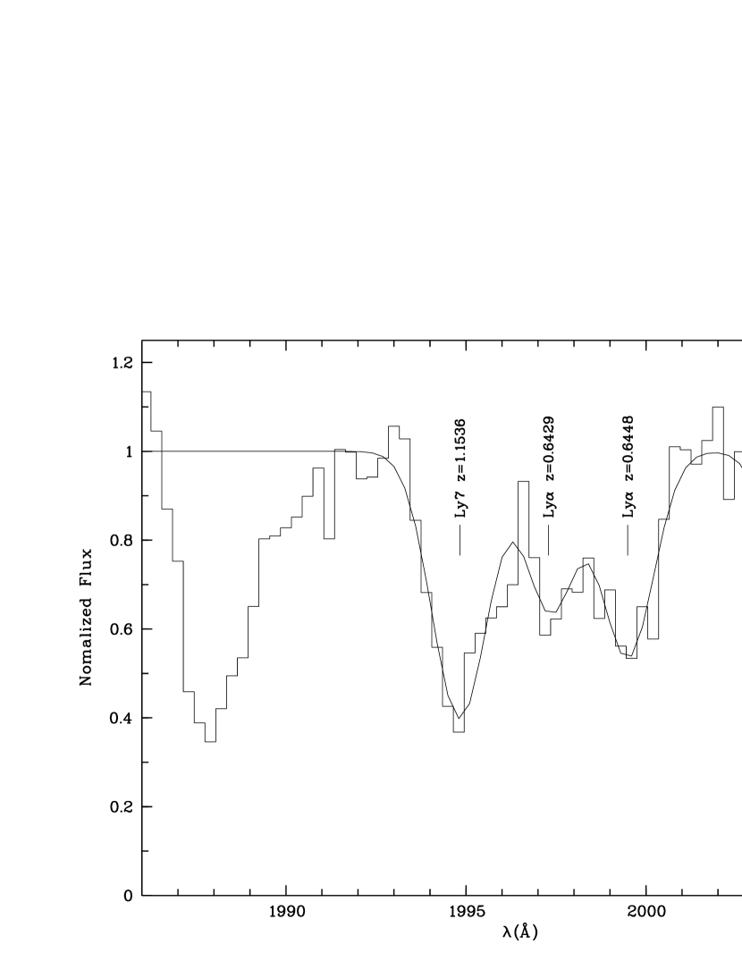
Figure 3: The deblending fit for the $z=0.6428$ Ly$\alpha$ line (second from the left) in the FOS spectrum. The blended lines are Ly$7$ at $z=1.1536$, Ly$\alpha$ at $z=0.6429$, and Ly$\alpha$ at $z=0.6448$. The lone feature at 2004.5 Å is Ly$6$ at $z=1.1536$, which is the redshift of a strong Mgii absorber.

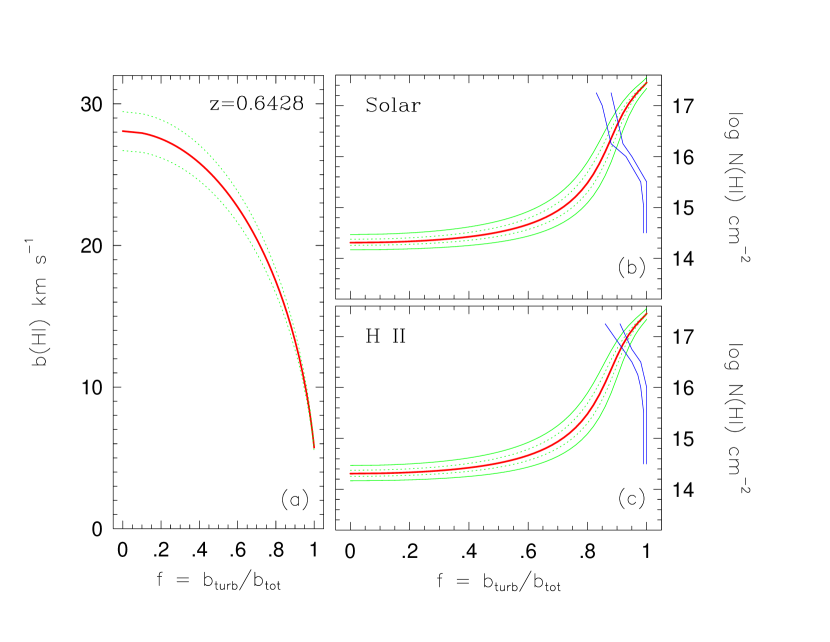
Figure 6: The $z=0.6428$ absorber properties — (a) The range of total Doppler $b$ parameters as a function of $f=b_{\rm turb}/b_{\rm tot}$. The dotted lines are the spread due the $1\sigma$ uncertainties in the measured Mgii $b_{\rm tot}$. — (b) and (c) The range of Hi column densities as a function of $f$. The thick solid curves are best values of $N({\hbox{{\rm H}\kern 1.00006pt{\sc i}}})$ based upon $b_{\rm tot}({\hbox{{\rm Mg}\kern 1.00006pt{\sc ii}}})$ and $W_{\rm r}({\hbox{{\rm H}\kern 1.00006pt{\sc i}}})$. The thin curves give the spread of $N({\hbox{{\rm H}\kern 1.00006pt{\sc i}}})$ based upon the $1\sigma$ uncertainties in $b_{\rm tot}({\hbox{{\rm Mg}\kern 1.00006pt{\sc ii}}})$ [inner] and $W_{\rm r}({\hbox{{\rm Ly}\kern 1.00006pt$\alpha$}})$ [outer]. The curves that originate in the lower right hand corners and rise upward and then to the left are the allowed locus of $f$ for a cloud model with a given $N({\hbox{{\rm H}\kern 1.00006pt{\sc i}}})$. Panel (b) is for a solar abundance patterns and (c) is for the Hii abundance pattern.

In the FOS spectrum, the Ly$\alpha$ absorption is the central line in a triple–blend feature. In Figure 3, we show the deblending fit. The adjacent lines in the blended feature are Ly$7$ at $z=1.1536$, and Ly$\alpha$ at $z=0.6448$. The lone feature at 2004.5 Å is Ly$6$ at $z=1.1536$, which is the redshift of a strong Mgii absorber studied elsewhere (Churchill et al. 1998). Though the fit is not unique, we have adopted the presented result, which yielded a rest–frame Ly$\alpha$ equivalent width of $W_{\rm r}=0.33\pm 0.03$ Å. Because of the low resolution of the FOS spectrum, we could not obtain estimates of the Hi column density and $b$ parameter directly from the data. There is no coverage at the expected position of the Lyman limit, so we cannot place an observed upper limit on $N({\hbox{{\rm H}\kern 1.00006pt{\sc i}}})$. The Ly$\beta$ falls just blueward of the Lyman limit at 1695 Å due to the $z=0.8596$ damped Ly$\alpha$ absorber, and thus cannot be detected. If the Hi and the Mgii arise in the same physical locations in the absorber, then the total Hi $b$ parameter is constrained to be $5.7\leq b({\hbox{{\rm H}\kern 1.00006pt{\sc i}}})\leq 29.8$ km s^-1 (see Figure 6a) including the spread introduced by the uncertainty in the measured $b_{\rm tot}({\hbox{{\rm Mg}\kern 1.00006pt{\sc ii}}})$. The lower limit corresponds to the case in which turbulence or bulk motions dominate the line broadening and the upper limit corresponds to a thermal motions scaling, $\sqrt{24}b_{\rm tot}({\hbox{{\rm Mg}\kern 1.00006pt{\sc ii}}})$. From the curve of growth, we have estimated that the inferred $b({\hbox{{\rm H}\kern 1.00006pt{\sc i}}})$ range translates to a neutral hydrogen column density range of $14.2\leq\log N({\hbox{{\rm H}\kern 1.00006pt{\sc i}}})\leq 17.6$ cm^-2. For this estimate, we have included the spread introduced by the uncertainty in the measured $W_{\rm r}({\hbox{{\rm Ly}\kern 1.00006pt$\alpha$}})$, which dominates over the uncertainty in $b_{\rm tot}({\hbox{{\rm H}\kern 1.00006pt{\sc i}}})$.

The FOS spectrum also covers several other transitions from a variety of species and over a wide range of ionization potentials. It is important to thoroughly check for the presence of absorption from these species and to place limits on their column densities when no absorption is detected. These limits may be useful for further constraining the chemical and ionization conditions of the absorber, even if the sensitivity level of the FOS spectrum is not very high. Thus, we have systematically searched the FOS spectrum for other transitions associated with the $z=0.6428$ absorber, using the detection method described by Schneider et al. (1993). Details of the search are presented in Appendix A and selected results are tabulated in Table 3.

4.2 The $z=0.9315$ System

In the right hand panels of Figure 2, the Mgii and Feii HIRES profiles are presented. Also shown (top panel) is the FOS spectrum, with the position of the corresponding Ly$\alpha$ line marked with a tick. Along with the Mgii doublet, the Feii $\lambda 2383$ transition was detected. The Feii $\lambda 2600$ transition may have been measurable as well, but its predicted location coincided by chance with that of the pen mark (i.e. “The Blob”) on the HIRES Tektronic’s CCD. The weaker Feii transitions were covered by the spectrum, but were not found to the 5$\sigma$ significance level. Their limits are consistent with the Feii $\lambda 2383$ detection.

In the lower panel of Table 2, the measured rest–frame equivalent widths, column densities and Doppler $b$ parameters are presented. The measured Mgii doublet ratio is $2.0\pm 0.1$, though it may be closer to 1.8, as we discuss below. The Mgii and the Feii lines are unresolved. For unresolved lines, it is difficult to accurately determine the column densities and $b$ parameters from profile fitting.

We have performed extensive VP fitting simulations of the Mgii doublet for this system. The constraints for adopting the best model were the measured Mgii $\lambda 2796$ equivalent width and the doublet ratio. Using the curve of growth, we explored a grid of column densities and $b$ parameters that were consistent with the measured equivalent width of the Mgii $\lambda 2796$ transition. The grid range was $12.1\leq\log N({\hbox{{\rm Mg}\kern 1.00006pt{\sc ii}}})\leq 14.2$ cm^-2, corresponding to $4.0\geq b({\hbox{{\rm Mg}\kern 1.00006pt{\sc ii}}})\geq 0.4$ km s^-1. The increments in column density were 0.1 dex. For each grid location, 500 spectra were simulated, convolved with the HIRES instrument spread function, sampled at the HIRES pixelization, and degraded to the signal–to–noise ratio of the observed data. The simulation output consisted of the Mgii $\lambda 2796$ equivalent width, the doublet ratio, and the VP column densities and $b$ parameters from minfit.

For $b\leq 1$ km s^-1, we found that we could not recover the measured equivalent width, nor the doublet ratio; they both decrease dramatically with decreasing $b$. This is due to the finite pixelization of HIRES. As $b$ is reduced, the line depth increases. As the pre–instrumentally broadened line width drops below that of a single pixel, saturation losses dominate. It could be argued that the measured equivalent width already reflects this (that the absorption is actually stronger than the measured value) and that larger equivalent widths should be explored. Fortunately, the VP fits recovered the input $b$ values to both high accuracy and precision over the full range explored. For $b\leq 1$ km s^-1, no matter the value of the equivalent width, the doublet ratio could never be made consistent with the data (within 3$\sigma$). For the lower limit on $b$, we adopted the criterion that the measured doublet ratio would be a 3$\sigma$ outlier in the distribution of simulated VP fits. For the upper limit on $b$, we adopted the criterion that the measured $b$ would be a $3\sigma$ outlier from the mode of the fitted $b$ distribution.

A caveat is worth noting. We also explored simulations in which the Mgii doublets were fit individually, rather than simultaneously. From this we concluded that the observed $\lambda 2803$ transition is likely compromised by a possible flat fielding artifact in its blue wing. This is consistent with the visual appearance of the data in comparison to the many simulated spectra and with the measured $\chi^{2}_{\nu}$ for the VP fits. The value of $\chi^{2}_{\nu}$ was 1.29 with $\nu=74$ when all three transitions were fit simultaneously. If just the Mgii doublet was fit, then $\chi^{2}_{\nu}=1.47$ with $\nu=51$. This value is dominated by the “poorer” fit to the $\lambda 2803$ transition, which by itself was $\chi^{2}_{\nu}=2.13$ with $\nu=24$. In contrast, the VP fit to just the $\lambda 2796$ transition yielded $\chi^{2}_{\nu}=0.97$ with $\nu=24$. The effect of this residual flux in the $\lambda 2803$ transition was to push the measured $b$ value down to 1.5 km s^-1, when the doublet was fit simultaneously. When the observed $\lambda 2803$ transition was omitted from the VP fit to the data, the resulting Mgii $b$ parameter was consistent with the mean of the simulations. Based upon these considerations, we have omitted the observed $\lambda 2803$ transition from the VP fit results; the measured $b$ parameter used for interpreting the simulations was obtained by a fit to the $\lambda 2796$ transition only. Since we have adopted the assumption that the observed $\lambda 2803$ transition has been compromised, we have adopted the “best” doublet ratio from the simulations, ${\hbox{\sc dr}}=1.8\pm 0.1$. This implies that the equivalent width of the $\lambda 2803$ line is slightly larger than that formally measured from the data. If the Mgii dr is 1.8, then rest frame $\lambda 2803$ equivalent width is $\sim 0.023$ Å.

The adopted VP column densities are $\log N({\hbox{{\rm Mg}\kern 1.00006pt{\sc ii}}})=12.24\pm 0.09$ cm^-2 and $\log N({\hbox{{\rm Fe}\kern 1.00006pt{\sc ii}}})=12.29\pm 0.08$ cm^-2. Their respective $b$ parameters $b_{\rm tot}({\hbox{{\rm Mg}\kern 1.00006pt{\sc ii}}})=2.2\pm 0.5$ km s^-1 and $b_{\rm tot}({\hbox{{\rm Fe}\kern 1.00006pt{\sc ii}}})=2.3\pm 1.6$ km s^-1. As with the $z=0.6428$, the value of $b_{\rm turb}/b_{\rm tot}$ for the system could be determined from the ratio of the atomic masses of iron and magnesium (see eq. [1] and eq. [3]), but the uncertainties are too large to directly place useful limits on $b_{\rm turb}$.

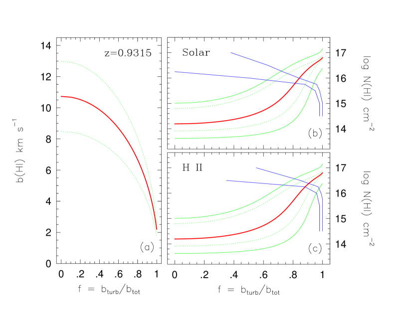
Figure 7: The $z=0.9315$ absorber properties. See caption for Figure 6.

Because of the low resolution of the FOS spectrum, we could not obtain estimates of the Hi column density and $b$ parameter directly from the data. However, the wavelength range over which the Lyman limit break could be observed is present in the spectrum at 1760.9 Å. There is no apparent flux decrement at the expected position of the break. However, the signal–to–noise ratio is low, $\sim 5$, and this places a $3\sigma$ limit of 1.6 on the flux ratio across the break. This corresponds to an upper limit $\log N({\hbox{{\rm H}\kern 1.00006pt{\sc i}}})\sim 16.5$ cm^-2. The Ly$\beta$ transition is covered at 1981.2 Å, but the region is dominated by the $z=1.1537$ Ly$9$ line at 1983.1 Å, so Ly$\beta$ does not provide a constraint on $N({\hbox{{\rm H}\kern 1.00006pt{\sc i}}})$. If the Hi and the Mgii arise in the same physical locations in the absorber, then the total Hi $b$ parameter is constrained to be $1.8\leq b({\hbox{{\rm H}\kern 1.00006pt{\sc i}}})\leq 13.0$ km s^-1 (see Figure 7a), including the spread introduced by the uncertainty in the measured $b_{\rm tot}({\hbox{{\rm Mg}\kern 1.00006pt{\sc ii}}})$. The lower limit corresponds to the case in which turbulence or bulk motions dominate the line broadening and the upper limit corresponds to a thermal motions scaling, $\sqrt{24}b_{\rm tot}({\hbox{{\rm Mg}\kern 1.00006pt{\sc ii}}})$. From the curve of growth, we have estimated that the inferred $b$ range translates to a neutral hydrogen column density range of $13.6\leq\log N({\hbox{{\rm H}\kern 1.00006pt{\sc i}}})\leq 16.5$ cm^-2, where we have adopted the upper limit from the Lyman limit break constraint. We have included the spread introduced by the uncertainty in the measured $W_{\rm r}({\hbox{{\rm Ly}\kern 1.00006pt$\alpha$}})$ in this estimate, which dominates over the uncertainty in $b_{\rm tot}({\hbox{{\rm Mg}\kern 1.00006pt{\sc ii}}})$.

As with the $z=0.6428$ absorber, we have systematically searched the FOS spectrum for other transitions associated with the $z=0.9315$ absorber using the detection technique described by Schneider et al. (1993). Details of the search are presented in Appendix A and selected results are tabulated in Table 3.

5 Modeling The Absorbers

In order to better understand the two absorbers, we have attempted to constrain their physical conditions, i.e. ionization and chemical conditions, non–thermal motions, and sizes. In particular, we are interested in the relationship between the ionizing flux, whether it is UVB or stellar/galaxy, and the inferred metallicity/abundance pattern. Taken together, constraints on these two quantities may reveal a great deal about the origin, history, and local environment of the absorbers.

We have modeled the absorbers as single–phase photoionized clouds using CLOUDY (Ferland (1996)). The clouds were assumed to have constant density and plane–parallel geometry. A grid of models were produced; for each model cloud the specified physical conditions were (1) the ionizing continuum shape and intensity, (2) the abundance pattern of the metals, and (3) the cloud neutral column density, $N({\hbox{{\rm H}\kern 1.00006pt{\sc i}}})$. These input quantities constitute the biggest uncertainties in modeling the absorbers. We used CLOUDY in optimize mode, in which the residuals between the model and the measured Mgii and Feii column densities were minimized. The two quantities allowed to vary (optimized) were (1) the metallicity of the assumed metal abundance patterns, and (2) the total hydrogen density, $n_{\rm H}$. For those ionization species for which column density upper limits were available, we applied the upper limits to the models.

5.1 The Photoionizing Sources

The two physical conditions within the absorbers that are the most telling of its formation history are their abundance pattern/metallicity and their photoionization source, either local stellar radiation or the UV background (UVB). In fact, the inferred chemical conditions are sensitive to the intensity and shape of the ionizing flux continuum. There are several scenarios and we address a few of the more obvious ones below.

5.1.1 The UVB Scenario

The two absorbers, whether associated with galaxies or not, may have photoionization conditions dominated by the UVB. To model this possibility, we have employed the UVB spectrum of Haardt & Madau (1996), where the intensity has been normalized at $z=0.5$ and $z=1.0$ for the $z=0.6428$ and the $z=0.9315$ absorbers, respectively. The Haardt & Madau UVB spectrum accounts not only for the UV flux emitted by QSOs and active galactic nuclei, but also for additional UV flux due to the reprocessing of soft X–rays (also from the QSOs and active galactic nuclei) in intervening absorbers at all redshifts.

The UVB spectra are shown in Figure 4, where only a select range of energies is shown. Also illustrated are the locations of the ionization potentials of a few key ionization species. The relevant ionization potentials that we are studying are all just above 1 Ryd, the ionization potential of Hi. Mgii and Feii have ionization potentials of 1.11 and 1.19 Ryd, respectively. The Cii ionization potential is 1.79 Ryd, and for Ciii is 3.52 Ryd. We mention Cii and Ciii because they probe the Hei edge, at 1.81 Ryd, and because we have limits on the Cii and Ciii absorption strengths.

5.1.2 The Stellar/Galaxy Scenario

These particular clouds could be embedded within galaxies that are aligned with the QSO on the plane of the sky (zero impact parameter), or they could be in the outskirts of the galaxies, i.e. in the extended halo or outer disks. In the latter scenario, the radiating stars can be treated as if they are all equidistant from the clouds. For any stellar/galaxy scenario, the number of stars and their spectral types, metallicities, and distances (quantities that determine the intensity and continuum shape of the ionizing flux) must be consistent with known objects in the universe.

The stellar/galactic UV flux could arise from a late–type solar–metallicity stellar population, which would give rise to a rapidly falling continuum with large Hi and Hei breaks. A “soft” spectrum is required by the observed upper limits on the high ionization species. A central question defining the scenario is: what level could stellar/galaxy flux be contributing to the UVB or be completely dominating the UVB? We have explored this question and have outlined the astrophysical principles in Appendix B. We constructed stellar/galactic CLOUDY grids that included three galactic spectral energy distribution models over a range of intensities and covered cases in which the stellar/galaxy flux was progressively stronger compared to the UVB and the case in which the UVB was locally “extinct”.

For the “dominant stellar–type” scenarios, in which the cloud could be near a dominant single star, we used Atlas stellar models (Kurucz (1991)). We produced a grid of optimized CLOUDY models using solar metallicity stars with $T_{\rm eff}=6,000$, 10,000, 15,000, 20,000, 30,000 K, and $\log g=4.4$ (the solar value). The spectral shape is not sensitive to the surface gravity, but is quite sensitive to the metallicity and the effective surface temperature. The continuum falls more rapidly toward the UV for solar metallicity stars, so these stars have “softer” continua than what would be expected in a low metallicity early–type galaxy.

To account for various metallicities and/or stellar populations, we also produced optimized CLOUDY grids using synthetic galaxy spectra. We used a 12 Gyr single–burst Worthey (1994) model with metallicity $[Z/Z_{\odot}]=-0.7$, and a somewhat younger Worthey model with a 8 Gyr single burst with metallicity $[Z/Z_{\odot}]=-2$. We also used a later–type galaxy model from Bruzual & Charlot (1993) with an exponentially decreasing star formation rate (SFR). This model is a 16 Gyr stellar population with 1% of the total star–forming mass in stars after a Gyr. These models serve to bracket a reasonable spread in galaxy spectral properties, given that an extreme scenario such as a star bursting galaxy can be ruled out for two reasons. First, a star burst spectrum would highly ionize the gas, giving rise to Siiv and Civ absorption out to a galactocentric distance of $\sim 100$ kpc (cf. eq. [2] of Giroux & Shull (1997)). In fact, we found that it was difficult to not produce too much Siiv and Civ even with the exponential SFR model. Second, images of the PKS 0454+039 field, in which point spread function removal of the QSO has been performed to high accuracy, reveal no unidentified luminous objects with the characteristics of a star bursting galaxy to a limiting $K$ magnitude of $\sim 20.5$.

5.2 The Metallicity and Abundance Pattern

Different chemical enrichment histories and different environments can give rise to a wide variety of chemical and ionization conditions. Given the possible high iron to magnesium abundance ratio in these absorbers, it is reasonable to assume that the clouds could arise in or near galaxies. Thus, to better understand the origin of the absorbers, we modeled three abundance patterns that are taken from typical gaseous objects in galaxies. The first is the solar abundance pattern, taken from Grevesse & Anders (1989) and Grevesse & Noels (1993).

In the interstellar medium (ISM), both magnesium and iron deplete onto dust grains (cf. Lauroesch et al. (1996); Savage & Sembach (1996)). Since the main constraints on the CLOUDY optimization are the measured Mgii and Feii column densities, we also considered the effects of heating and cooling by grains and the dust depleted abundance patterns of two common interstellar environments. We used the Hii abundance depletion pattern taken from Baldwin et al. (1991), Rubin et al. (1991), and Osterbrock, Tran, & Vielleux (1992). For this abundance pattern we used the “large–R” grains (Baldwin et al. (1991)), which are characterized by a more or less grey UV extinction. Like the solar abundances, the Hii pattern, which has $[\hbox{Mg/Fe}]=-0.07$, provides a good template for an iron–group enriched chemical evolution history.

We have also explored the possibility that these absorbers may actually be $\alpha$–group enhanced. Thus, we used the abundance patterns reported by Cowie & Songaila (1986) for the cold and warm phases of the ISM. This pattern is characterized by $[\hbox{Mg/Fe}]=1.23$, and overall enhanced $\alpha$–group elements. The dust grains used in these ISM models are a mixture of the graphite and silicates.

The presence of grains also effects the cooling and heating balance, and thus the ionization balance, of the clouds. As mentioned, the metallicity, or the scaling factor of the input abundance pattern for elements heavier than helium, was allowed to vary. As the metallicity in a cloud is increased by factors of a few, the cooling rates are dramatically increased and the cloud equilibrium temperatures drop significantly. For some clouds, the optimal metallicity was 10 to 100 times the initial input and the cloud equilibrium temperature in the 100 K range.

5.3 Turbulent and/or Bulk Motions

It is not possible to obtain a direct determination of the Hi column densities for the two Mgii absorbers. For each, the extreme range of plausible Hi column densities can be estimated from the measured Mgii $b$ parameter for the assumption of a thermal line broadening [lower $N({\hbox{{\rm H}\kern 1.00006pt{\sc i}}})$ limit] or turbulent broadening [upper $N({\hbox{{\rm H}\kern 1.00006pt{\sc i}}})$ limit]. The range turns out to be large, $13.8\leq\log N({\hbox{{\rm H}\kern 1.00006pt{\sc i}}})<17.0$ cm^-2, when the uncertainties in $b({\hbox{{\rm H}\kern 1.00006pt{\sc i}}})$ and $W_{\rm r}({\hbox{{\rm Ly}\kern 1.00006pt$\alpha$}})$ are considered. We have modeled clouds with $\log N({\hbox{{\rm H}\kern 1.00006pt{\sc i}}})=14.50$, 15.50, 15.75, 16.00, 16.25, 16.50, 16.75, 17.00, and 17.50 cm^-2. As will be shown, there were no $\log N({\hbox{{\rm H}\kern 1.00006pt{\sc i}}})\leq 15.75$ cm^-2 cloud models consistent with the data. Since, for a known equivalent width, the curve of growth provides a direct relationship between the Hi column density and $b$ parameter, both quantities should be considered for constraining viable cloud models. Thus, we have developed a technique to further constrain the acceptable model cloud properties using the relationship between the turbulent and thermal line broadening mechanisms.

Using the equilibrium temperature of the CLOUDY models and the $b_{\rm tot}$ of Mgii, one can narrow parameter space to those models that are self–consistent in $b_{\rm turb}/b_{\rm tot}$, temperature, and $N({\hbox{{\rm H}\kern 1.00006pt{\sc i}}})$. Here, $b_{\rm turb}$ is the non–thermal contribution to the line broadening. Assuming the contributions are Gaussian, $b_{\rm tot}$ is written,

$$b_{\rm tot}^{2}=b_{\rm therm}^{2}+b_{\rm turb}^{2}=\frac{2kT}{m}+b_{\rm turb}^{2},$$ (1)

where $T$ is the equilibrium kinetic temperature, and $m$ is the ion mass. In reality, non–thermal motions are not expected to be Gaussian (see discussion in §5.5), so eq. [1] is simply a parameterization of the relative contributions. Defining $f=b_{\rm turb}/b_{\rm tot}$, the kinetic temperature of the cloud is written,

$$T\simeq 1450\left(1-f^{2}\right)b^{2}_{\rm tot}({\hbox{{\rm Mg}\kern 1.00006pt{\sc ii}}})\quad\hbox{K}.$$ (2)

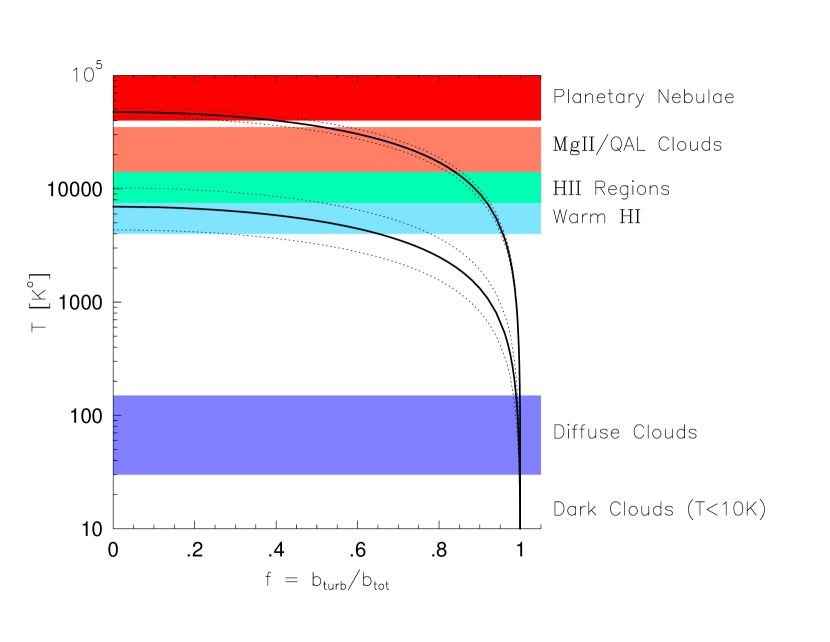
Figure 5: The inferred temperature of the $z=0.6428$ absorber (upper curves) and of the $z=0.9315$ absorber (lower curves) as a function of the fraction of the measured Mgii $b$ parameter due to possible turbulence, $f=b_{\rm turb}/b_{\rm tot}$. The uncertainties in $T$, based upon the $1\sigma$ uncertainties in the Mgii $b_{\rm tot}$, are given by the dotted curves. The shaded regions give the typical range of $T$ for various objects in the Galactic ISM and for Mgii QSO Absorption Line (Mgii/QAL) clouds at $z\sim 1$. The observed absorbers are consistent with Mgii/QAL clouds, Hii Regions, and Warm Hi clouds (see text).

In Figure 5, the predicted kinetic temperature for absorbers are shown as a function of $f$. Schematically superimposed are the kinetic temperature ranges of typical gaseous structures in the Galaxy (Savage & Sembach (1996); Fitzpatrick & Spitzer (1994); Osterbrock (1989); Spitzer (1978)). Also shown is the inferred range of Mgii absorbers, as observed using QSO absorption lines (Churchill 1997a ; Churchill et al. 1998). This diagram is discussed further in §6.

The $b$ parameter of each species is required in order to obtain its estimated column density from the curve of growth. Usage of the curve of growth method is consistent with our assumption of single–phase clouds, given that the velocity structure of the low ionization absorption profiles are not complicated and are suggestive of a single absorbing component. Assuming that all species are subject to the same thermal and non–thermal conditions, the total Doppler $b$ parameter of any species, X, can be obtained from,

$$b_{\rm tot}({\rm X})=\left\{\frac{A_{\rm Mg}}{A_{\rm X}}\left(1-f^{2}\right)+f^{2}\right\}^{1/2}b_{\rm tot}({\hbox{{\rm Mg}\kern 1.00006pt{\sc ii}}})\quad\hbox{\hbox{km~{}s${}^{-1}$}},$$ (3)

where $A$ is the nucleon number ($A_{\rm Mg}=24$).

5.4 Application of Constraints to Models

In the absence of direct measurements of $N({\hbox{{\rm H}\kern 1.00006pt{\sc i}}})$, the most acceptable cloud models are those that are self–consistent in that their $N({\hbox{{\rm H}\kern 1.00006pt{\sc i}}})$, temperatures, and $f$ are simultaneously consistent with those allowed by the data. With the above formalism in hand, the application for constraining a given cloud model is as follows: The range of acceptable $f$ values parameterize the clouds, and give the inferred non–thermal component to the line broadening. The range is determined from the model cloud kinetic temperature, $T$, using a modified version of eq. [2],

$$f_{(\mp)}=1-\frac{1}{b_{(\pm)}^{2}({\hbox{{\rm Mg}\kern 1.00006pt{\sc ii}}})}\left(\frac{T}{1450}\right),$$ (4)

where $b_{(\pm)}({\hbox{{\rm Mg}\kern 1.00006pt{\sc ii}}})=b_{\rm tot}({\hbox{{\rm Mg}\kern 1.00006pt{\sc ii}}})\pm\sigma_{b}$. The cloud temperature was taken as a simple average, given that the model clouds are constant density by definition. For clouds with $N({\hbox{{\rm H}\kern 1.00006pt{\sc i}}})\leq 16.5$ cm^-2, the temperature was constant as a function of depth. For the higher column density clouds, ionization and temperature structure was present, but by no more than 10%. Eq. [3] was then used to obtain the inferred $b_{\rm tot}({\hbox{{\rm H}\kern 1.00006pt{\sc i}}})$, as illustrated in Figure 6a and Figure 7a. Using curve of growth analysis, the range of acceptable hydrogen column densities is obtained from the measured Ly$\alpha$ equivalent width (and its uncertainty) and the range of acceptable $b_{\rm tot}({\hbox{{\rm H}\kern 1.00006pt{\sc i}}})$.

5.5 Caveats Regarding the Model Design

The quoted upper limits on the ionization species covered by the FOS spectrum were estimated assuming a single–phase isothermal cloud. There are a priori reasons that we have adopted this assumption. First, if the absorbers are Ly$\alpha$ clouds that are pressure confined by a warmer, more tenuous medium (more than one thermal phase giving rise to absorption), they cannot be heated by the UVB (Guilbert, Fabian, & McCray (1983); Donahue & Shull (1991)). On the other hand, under the assumption of photoionization by the UVB, a very low ionization parameter, $U=n_{\gamma}/n_{\rm H}\leq 10^{-3.5}$, is required in order for the absorbing gas to give rise to $N({\hbox{{\rm Fe}\kern 1.00006pt{\sc ii}}})\sim N({\hbox{{\rm Mg}\kern 1.00006pt{\sc ii}}})$ (Bergeron & Stasińska (1986); Churchill 1997a ). Therefore, for UVB photoionization, clouds giving rise to the Mgii and comparable Feii absorption must have low ionization conditions. If strong Civ and Siiv were to arise in a UVB photoionized absorber exhibiting $N({\hbox{{\rm Mg}\kern 1.00006pt{\sc ii}}})\simeq N({\hbox{{\rm Fe}\kern 1.00006pt{\sc ii}}})$, then the abundance pattern would need to be very different from solar, with a $1-2$ dex enhancement of iron or decrement of magnesium. Common chemical evolution paths do not give rise to this type of abundance pattern.

Nonetheless, the possibility remains that the absorbers could be multiphased in their ionization structures (perhaps they are not pressure confined or are ionized by stellar/galactic flux), so that the measured Ly$\alpha$ equivalent width may be due to a kinematic complex of clouds in which only one is giving rise to the observed Mgii and Feii absorption. As reported by SC96, Ly$\alpha$ clouds at $z=2.5$ are seen to exhibit kinematic structure in Civ absorption, with the highest velocity components more highly ionized. They suggest that this arises due to layered stratification in coalescing clouds. If this were the case for the low redshift absorbers reported here, then the upper limits provided by the FOS spectrum would not apply to this higher ionization phase; the limits would be lower than those quoted above on account of the expected larger $b$ parameters.

If a high ionization phase exists in either absorber, it has apparently not been detected in the FOS spectrum, suggesting that either its ionization conditions or abundance patterns are not giving rise to strong absorption lines. For the ionization conditions to give rise to a multiphase absorber, the neutral hydrogen column density would need to approach the Lyman limit value of $10^{17.3}$ cm^-2 to provide shielding to the low ionization phase. If there is no surrounding hot phase associated with these absorbers, it might be difficult to understand them in terms of pressure confined clouds; they could either be gravitationally bound or not be in dynamical equilibrium. Observationally, some ambiguity still remains for the detection of Civ and Siv in the $z=0.6428$ absorber. This uncertainty could be checked by higher resolution and higher signal–to–noise ratio observations with STIS/HST.

A main point here is that the physical region of the absorbers giving rise to the Mgii and Feii must have insignificant Civ and Siiv abundances. A second main point is that the estimated Hi column density in this region would be an upper limit to this low ionization phase, since some fraction of Hi would be arising in the high ionization phase as well. Unless the path length through a possible high ionization phase is far greater than that of the low ionization phase, the estimated ranges of the Hi column densities for the two absorbers cannot be significantly incorrect.

There is also the possibility that the spatial alignment of the neutral hydrogen in these absorbers may not directly coincide with that of the ionized magnesium (ionization structure), since the ionization potential of Mgii and Hi are slightly different (P. Boissé, private communication ). Again, this would imply that the Hi column densities in the region where Mgii and Feii are giving rise to absorption is smaller than the estimated values.

The presence of dust can effect the modeling in two ways. First, for the model clouds using the Hii/ISM dust–depleted abundance pattern, there is a breakdown in the inferred metallicity when the temperatures are below $T\sim 1000$ K. The condensation temperature (the temperature at which 50% of an element is removed from the gas phase due to depletion) of both magnesium and iron is $\sim 1300$ K. This means that these cool clouds would have a significantly higher depletion than the warmer clouds, and this has not been accounted for in the CLOUDY modeling. The implication is that the optimized metallicity is in fact an underestimate of the gas–phase abundances, given that the depletion would be larger than that input into the model. Second, if dust is present, it can seriously modify the intensity and shape of the incident UV spectrum, which would have implications for the inferred source of the radiation from the photoionization models. We discuss this point further in §6.3.

Central to the model interpretation is the assumption that the line broadening is governed by Gaussian distribution functions for the particle velocities. N–body simulations with hydrodynamics (Norman et al. (1997); Davé et al. (1997); Zhang et al. (1997)) have shown that the absorbers are filamentary structures and that the concept of an absorbing “cloud” is not altogether valid. Often, the simulations result in gas which is collapsing towards (or expanding along) a filament; this results in hydrodynamic features and shocks in which the distribution function of velocities is not Gaussian. If the Mgii absorption profiles give any indication of the velocity distribution function, then the absorbers are not inconsistent with a Gaussian; in fact, very quiescent gas is suggested by the HIRES profiles.

A final caveat is that we did not include turbulence physics in the CLOUDY models (only micro–turbulence and not bulk motions could have been modeled using CLOUDY). Thus, turbulence is not treated self consistently within the framework used to infer the absorber physical conditions. The inclusion of turbulence would result in an additional pressure source, which would effect the balance between the model cloud density and its depth. However, the model cloud densities were allowed to vary in an optimized fashion, and since the cloud depth is adjusted with each equilibrium calculation the pressure adjustment has little effect. The second consequence of modeling turbulence is that the line–center optical depths of absorption transitions decrease, while they increase in the line wings. However, since the majority of the model clouds in our grids were optically thin to neutral hydrogen, any change in the line profile shape has little effect on the model cloud equilibrium.

6 Model Results

In the final analysis, only the scenario in which the model clouds are photoionized by the UVB was both astrophysically plausible and consistent with the data. Here, we focus on the results for the UVB scenario with the solar and Hii/ISM abundance patterns and then address to what level the stellar/galactic scenarios can be ruled out as viable ionizing sources. We defer discussion of the implications of the model results until §7.

The optimized metallicities and densities are given for both abundance patterns in Tables 4 and 5. Cloud models with the $\alpha$–group enhanced abundance pattern (Cowie & Songaila (1986)) did not converge within the allowed uncertainties in the Mgii and Feii column densities. Thus, we conclude that neither the $z=0.6428$ nor the $z=0.9315$ absorber have $\alpha$–group enhanced abundance patterns. This implies a gas–phase $[\hbox{Fe/H}]\geq-1$ (Lauroesch et al. (1996); Savage & Sembach (1996)), and possibly iron–group enrichment by Type Ia SNe, though this remains somewhat controversial (Gibson et al. 1997). The $N({\hbox{{\rm H}\kern 1.00006pt{\sc i}}})$ versus $f$ parameter space is illustrated in Figures 6 and 7 for the data and for the model clouds. The adopted ranges for the absorber Hi column densities are defined by the overlap of the allowed ranges constrained by the data and by the CLOUDY models. Interestingly, the results indicate that the clouds have a substantial non–thermal line broadening (i.e. they are turbulent or are undergoing differential bulk motions). However, it is striking that the Mgii profiles reveal a velocity dispersion of only a few km s^-1. This provides a counter example to the expected large $b$ parameters if the gas was not dynamically settled (as found in hydrodynamic simulations of the Ly$\alpha$ forest). The very quiet nature of these absorbers indicate that our assumption of a well defined temperature for a settled gas “cloud” is well founded. A possible, though unlikely, counter example would be if the absorbers were streaming filaments seen perpendicular to their elongation and streaming motion.

Shown in Figure 5 are the predicted kinetic temperatures of the absorbers as a function of $b_{\rm turb}/b_{\rm tot}$. Temperature and turbulence limits may provide clues to the nature of the absorbing gas when the range of inferred properties are compared to gaseous objects typically found in galaxies. Planetary nebulae have $T\geq 40,000$ K (Osterbrock (1989); Spitzer (1978)). If the $z=0.6428$ absorber has $f\leq 0.4$, then its inferred temperature is consistent with that of a planetary nebulae. Typical expansion velocities of these objects have line widths of $\sim 20-30$ km s^-1 (Osterbrock (1989)). Since the Mgii and Feii Doppler parameters would also reflect the expansion velocities, it is highly unlikely that the $z=0.6428$ absorber arises in a planetary nebula. For $0.4\leq f\leq 0.9$, the $z=0.6428$ absorber temperature is consistent with that of individual clouds in complex Mgii systems (Churchill 1997a ; Churchill et al. 1998). Both absorbers are consistent with the temperature range of Hii regions and warm Hi clouds, $7000\leq T({\hbox{{\rm H}\kern 1.00006pt{\sc ii}}})\leq 14,000$ K and $4000\leq T({\hbox{{\rm H}\kern 1.00006pt{\sc i}}})\leq 7000$ K, respectively (Fitzpatrick & Spitzer (1994); Osterbrock (1989); Spitzer (1978)). For the $z=0.9315$ absorber, the inferred $b_{\rm turb}/b_{\rm tot}$ would be $f\leq 0.8$, and for the $z=0.6428$ absorber $f$ would be confined to the narrow range $0.90\leq f\leq 0.95$. For these $f$ values, the non–thermal broadening would be roughly $b_{\rm turb}({\hbox{{\rm Mg}\kern 1.00006pt{\sc ii}}})\leq 5$ km s^-1 and $\leq 2$ km s^-1 for the $z=0.6428$ and the $z=0.9315$ absorber, respectively. The typical sound speeds in Hii and Hi clouds are $\sim 10~{}{\hbox{km~{}s${}^{-1}$}}$ (Spitzer (1978)). If these absorbers are Hii or Hi clouds similar to those found in the Galaxy, the line of sight non–thermal broadening is well below that expected for propagating disturbances in the clouds. If the absorbers are dominated by turbulent motions ($f>0.98$), then they must have $T\leq 150$ K. Diffuse ISM clouds have typical temperatures in the range $30\leq T\leq 150$ K (Spitzer (1978)). In this regime, it would be more likely that the broadening was dominated by bulk flows rather than internal turbulence, given that the turbulent motion would propagate at the $\sim 0.1$ km s^-1 sound speed typical of diffuse clouds (Spitzer (1978)).

6.1 The $z=0.6428$ Absorber Properties

Assuming the solar abundance pattern, the neutral hydrogen of the $z=0.6428$ model cloud is in the range $16.3\leq\log N({\hbox{{\rm H}\kern 1.00006pt{\sc i}}})\leq 16.8$ cm^-2. The range of $b_{\rm turb}/b_{\rm tot}$ is $0.85\leq f\leq 0.93$, which correspond to the kinetic temperatures $13,000\geq T\geq 6500$ K. The metallicity and model cloud density are $-0.2\geq[Z/Z_{\odot}]\geq-0.7$, and $0.01\leq n_{\rm H}\leq 0.02$ cm^-3, for the range of $N({\hbox{{\rm H}\kern 1.00006pt{\sc i}}})$. For the Hii abundance pattern, the inferred neutral hydrogen column density is slightly higher, in the range $16.7\leq\log N({\hbox{{\rm H}\kern 1.00006pt{\sc i}}})\leq 17.2$ cm^-2. The range of $b_{\rm turb}/b_{\rm tot}$ is $0.90\leq f\leq 0.95$, making this cloud kinetic temperature somewhat lower than the solar abundance model. The density and metallicity are $n_{\rm H}\simeq 0.008$ cm^-3 and $+0.4\geq[Z/Z_{\hbox{{\rm H}\kern 0.70004pt{\sc ii}}}]\geq 0.0$, for the range of $N({\hbox{{\rm H}\kern 1.00006pt{\sc i}}})$. It could be that this cloud has very enhanced metallicity with an Hii abundance pattern, but this is a far reaching suggestion given the range allowed by the solar abundance pattern. Still, the cloud is inferred to have gas–phase $[\hbox{Fe/H}]\geq-1$.

These model clouds are difficult to understand in terms of objects typical of the Galactic disk or the Magellanic Clouds. For one, the typical $N({\hbox{{\rm H}\kern 1.00006pt{\sc i}}})$ observed in Galactic objects is $\log N\geq 19.5$ cm^-2 (Savage & Sembach (1996)), two or more orders of magnitude greater than what is inferred for this absorber. Second, the typical density of $T\sim 10,000$ K clouds (warm low density medium) is $\left<n_{\rm H}\right>\sim 0.2$ cm ^-3 (Spitzer (1978)), which is higher than allowed by the optimal models. Third, the inferred gas–phase abundances in the the warm and cool disk are $[\hbox{Fe/H}]\sim-1.1$ and $\sim-2.1$, respectively (Savage & Sembach (1996)). These fall well below those predicted by the models. However, the metallicity range of the solar abundance pattern model is consistent with $[\hbox{Fe/H}]\sim-0.6$ found for the Galactic Halo.

6.2 The $z=0.9315$ Absorber Properties

The $z=0.9315$ model cloud appears to have a high gas–phase metallicity, whether it be super solar or an enhanced Hii pattern. Assuming the solar abundance pattern, the neutral hydrogen is in the range $15.8\leq\log N({\hbox{{\rm H}\kern 1.00006pt{\sc i}}})\leq 16.3$ cm^-2. Note that this is consistent with the upper limit of 16.5 cm^-2 inferred from the lack of a Lyman limit break in the FOS spectrum. The range of $b_{\rm turb}/b_{\rm tot}$ is $0.62\leq f\leq 0.94$, which correspond to the kinetic temperatures $4600\geq T\geq 870$ K. The metallicity and model cloud density are $+0.7\geq[Z/Z_{\odot}]\geq+0.1$, and $0.2\leq n_{\rm H}\leq 0.4$ cm^-3, for the range of $N({\hbox{{\rm H}\kern 1.00006pt{\sc i}}})$. The optimal solar abundance model cloud is relatively dense with up to five times solar abundance. The inferred $[\hbox{Fe/H}]$ is even greater for the Hii abundance pattern model. The neutral hydrogen column density is slightly higher, in the range $16.0\leq\log N({\hbox{{\rm H}\kern 1.00006pt{\sc i}}})\leq 16.5$ cm^-2 (also consistent with the lack of a Lyman limit). The range of $b_{\rm turb}/b_{\rm tot}$ is $0.75\leq f\leq 0.97$, which corresponds to the kinetic temperatures $3300\geq T\geq 450$ K. There is an inversion in the cooling curve at $T\sim 2000$ K, which implies that this absorber cannot be stable across the full range of allowed temperatures. It must either be a few thousand degrees or several hundred degrees. The density and metallicity are $n_{\rm H}\simeq 0.1$ cm^-3 and $+1.6\geq[Z/Z_{\hbox{{\rm H}\kern 0.70004pt{\sc ii}}}]\geq+0.7$, for the respective $N({\hbox{{\rm H}\kern 1.00006pt{\sc i}}})$. This is a metallicity enhancement of five to 40 times over the typical values seen in Galactic Hii regions (Baldwin et al. (1991); Rubin et al. (1991); Osterbrock et al. 1992). To date, no other intervening QSO absorption system with such a high metallicity has been reported.

6.3 Why the Stellar/Galaxy Scenarios Fail

In what follows, we discuss the difficulties with the stellar/galaxy scenarios. The constraints were a trade off between the number of stars, or their number density, and the stellar population. The former is constrained by astrophysics, assuming a non–extreme stellar environment, and by the imaging data. The latter is constrained by the absorption line data, which have limited the UV ionizing flux to late–type stars and/or early–type galaxies.

First, consider the case in which the stellar/galactic flux contributes to the UVB intensity. In order for a stellar/galactic contribution to modify the properties of a UVB model cloud, the stellar/galactic flux must exceed the UVB at $\geq 1$ Ryd, particularly in the regions $1\leq h\nu\leq 1.2$ Ryd (from the Hi edge up to and including the Feii ionization potential). As outlined in Appendix B, if the stellar population is dominated by A0III and A0V stars, this requires $\sim 10^{12}$ stars confined to a region of space $\sim 1$ kpc in radius. This implies a stellar number density $n_{\ast}\geq 500$ stars pc^-3, which is five orders of magnitude greater than the density of A0V stars in the solar neighborhood (Allen (1981)). The required number density increases dramatically for later spectral types. If, on the other hand, the stars are dominated by early–type B0V (B0I,III) stars, then $\sim 10,000$ (1000) stars would be required in a volume of radius 1 kpc. For the main sequence stars, this corresponds to a number density about 100 times greater than that of the solar neighborhood (Allen (1981)). Only O stars can provide the UV flux necessary to match the UVB at 1 Ryd and have a number density of stars consistent with that of a typical galaxy environment. However, early–type stars give rise to high ionization absorption properties, especially Ciii, Civ, and Siiv, so that the model cloud conditions are not consistent with the data.

The 12 Gyr $[Z/Z_{\odot}]=-0.7$ Worthey (1994) model is characterized by a steep continuum slope with $\Delta\log\nu f_{\nu}\sim-5$ from 1 to 1.2 Ryd. This continuum shape is a smooth continuation of the Hi edge, so that this galaxy model had to have $\nu f_{\nu}\geq 10^{8}$ times that of the UVB at 5500 Å before affecting the model cloud properties. Based upon the arguments presented in Appendix B, for the expected distribution of main sequence and giant stars in these galaxies (Worthey (1994)), the stellar number densities would be extreme, $N_{\ast}\geq 10^{2}$ stars pc^-3, or $\sim 10^{12}$ stars within a kpc. Even under these extreme conditions, the 12 Gyr Worthey models yielded $[\hbox{Fe/H}]\geq-1$.

The 8 Gyr Worthey model with metallicity $[Z/Z_{\odot}]=-2$ is characterized by a continuum with a smaller Hi edge of $\Delta\log\nu f_{\nu}\sim-2$ at 1 Ryd and a power law with $\sim\nu^{-7}$ out to $\sim 1.5$ Ryd (this is steep but not nearly as steep as the 12 Gyr model). The flux must be elevated to $\nu f_{\nu}\geq 10^{5}$ times that of the UVB at 5500 Å before affecting the model cloud properties. As the flux, $\nu f_{\nu}(0.17)$, is increased above $\sim 10^{4}$ ergs cm^-2 s^-1, the ratio $N({\hbox{{\rm H}\kern 1.00006pt{\sc i}}})/N({\hbox{{\rm H}\kern 1.00006pt{\sc ii}}})$ very quickly changes from unity to $\sim 10^{-5}$; the model cloud becomes highly ionized and the limits on Ciii and/or Civ are exceeded (depending upon the specific absorber). To adopt the idea that the 8 Gyr Worthey galaxy is contributing to the ionization conditions, we would be forced to accept a very narrow range of acceptable $\nu f_{\nu}(0.17)$ arising from the galaxy. This range implies the absorbers would be embedded in the galaxy itself (zero impact parameter), with an extremely unrealistic number of stars. Such a scenario is ruled out.

The exponential SFR spectrum of Bruzual & Charlot (1993) has a continuum shape at $1-3$ Ryd that is similar to the Haardt & Madau UVB spectrum. Thus, as the galactic spectrum is slowly increased over the UVB, the model cloud properties adjust such that the ionization parameter is held constant (the cloud density increases, but the metallicity and temperature do not change). At $\nu f_{\nu}(0.17)\sim 0.1$ ergs cm^-2 s^-1, there is a slow decrease in the ratio $N({\hbox{{\rm H}\kern 1.00006pt{\sc i}}})/N({\hbox{{\rm H}\kern 1.00006pt{\sc ii}}})$; the model cloud becomes progressively highly ionized. The dominant ionization species of magnesium and iron are then Mgiii and Feiii, respectively, and the Civ and Siiv column densities exceed the limits allowed by the data. The exponential SFR galaxy of Bruzual and Charlot is not a viable photoionizing source. The galaxy flux makes little modification to the inferred cloud properties (does not modify UVB only models) for a large range of intensities; once it does modify the UVB models, the cloud properties are inconsistent with the data.

Now, consider the case in which the stellar/galactic flux is dominant. We examined this by excluding the Haardt & Madau UVB from the incident flux. This would require environments that are more extreme than those presented above, or that are shielded from the UVB but not from the stellar flux. Is it possible that dust extinction could be playing a role? For a dust absorption/scattering cross section of $\sigma(\hbox{1~{}Ryd})\sim 10^{-22}$ cm^-2 (Mathis, Rumpl, & Nordsieck (1977)), the total hydrogen column density [$N({\hbox{{\rm H}\kern 1.00006pt{\sc i}}})+N({\hbox{{\rm H}\kern 1.00006pt{\sc ii}}})+2N({\rm H}_{2})$] required for $\tau_{\rm dust}\sim 3$ at 1 Ryd is $\log N\sim 22.5$ cm^-2. Given the upper limits on $N({\hbox{{\rm H}\kern 1.00006pt{\sc i}}})$ for the absorbers, this implies highly ionized gas with $N({\hbox{{\rm H}\kern 1.00006pt{\sc i}}})/N_{\rm tot}({\rm H})\geq 10^{-5}$. In all our model clouds, the fraction of molecular hydrogen never increased above $f({\rm H}_{2})\leq 10^{-6}$.

In principle, one could imagine an environment in which the absorbing gas is embedded in a late–type dwarf galaxy that itself is enshrouded in dust. This scenario provides the steep continuum above 1 Ryd while not requiring the spectrum intensity to be elevated above the UVB. For some models it was possible to achieve $\log N({\hbox{{\rm H}\kern 1.00006pt{\sc ii}}})\simeq 22.5$ cm^-2, but even with no competition from the UVB, these shielded models required high $\nu f_{\nu}(0.17)$. Again, as outlined in Appendix B, this implies unrealistic stellar densities. It is not simply a matter of the continuum slope, but also the intensity that dictates the cloud ionization conditions. Interestingly, these models produced very low metallicities, with $[Z/Z_{\odot}]\sim-3$. All of the above stellar/galaxy models represent our failed attempt to locate a place in parameter space consistent with low metallicity clouds.

7 Discussion

Based upon the success rate of finding two Mgii absorbers out of 28 Ly$\alpha$ absorbers along the PKS 0454+039 line of sight, we must conclude that the two absorbers are unique in some manner with respect to the Ly$\alpha$ forest at large. We note, as mentioned in §4, that not a great deal can be quantified about the range of metallicities in the Ly$\alpha$ forest at $z\leq 1$ based upon our upper limits on the Mgii column densities. However, if our assumption of $b\sim 30$ km s^-1 is not applicable, as found for the two Mgii absorbers, then our quoted estimates in the range of metallicities would be quite wrong. In fact, given that the upper limits on the metallicity are super–solar for the $W_{\rm r}({\hbox{{\rm Ly}\kern 1.00006pt$\alpha$}})\leq 0.3$ Å absorbers, and that it is not expected that many of the absorbers are super–solar, we are lead to suggest that either the $b$ parameters of the $W_{\rm r}({\hbox{{\rm Ly}\kern 1.00006pt$\alpha$}})\leq 0.3$ Å absorbers are significantly smaller than 30 km s^-1 or the objects do not have a Gaussian velocity distribution (simple curve of growth techniques are not applicable). It could be that the uniqueness of the two Mgii absorbers is that they are dynamically settled and have a small velocity dispersion.

Other possibilities for the uniqueness of the Mgii absorbers, are:

(1) Their ionization conditions are different: If the chemical enrichment histories of these absorbers are typical of Ly$\alpha$ forest clouds, then it might be inferred that their ionization conditions are governed by a local UV flux rather than the UVB. However, our models lead us to conclude that there is nothing “special” about the photoionization conditions of these clouds; they are best described as being photoionized by the UVB. There is no evidence to suggest that these clouds are collisionally ionized.

(2) Their chemical conditions are different: If the ionization source is no different than that ionizing the other 26 Ly$\alpha$ systems we searched, then we are led to infer somewhat unique chemical enrichment histories for these two absorbers. If these absorbers are IGM/Ly$\alpha$ clouds, in that they are not associated with galaxies, then the low metallicity results of SC96 at higher redshift do not support the notion that these two absorbers have undergone typical IGM chemical enrichment. In other words, these two absorbers are not consistent with the picture in which the IGM was enriched at high redshift by a single burst of Population III stars that left the Ly$\alpha$ forest $\alpha$–group enhanced with $[\hbox{Fe/H}]\leq-2$. Thus, these absorbers could constitute a metal–rich minority of the IGM/Ly$\alpha$ population (less than $\sim 10$%). It then becomes a question of understanding what environments and evolutionary histories give rise to high metal content in some Ly$\alpha$ clouds. It is already known that at least some fraction of the Ly$\alpha$ forest at $z<1$ are associated with galaxies (Le Brun et al. (1996); Lanzetta et al. (1995); Bowen et al. 1996).

(3) Both their ionization and chemical conditions are different: Inferring the chemical content of ionized absorbers requires ionization corrections that are uncertain. In the case of photoionization, the inferred conditions of the clouds are very sensitive to both the intensity and shape of the ionizing continuum. We have explored this interplay between the chemical content of the clouds and the properties of the UV ionizing flux, and have concluded with some certainty that the ionizing field for the two absorbers is constrained to have slope and intensity consistent with the UVB. This is tantamount to saying that it is only the chemical conditions that are inferred to be unique in the two absorbers.

Overall, it is difficult to understand these absorbers in terms of the classic picture of Ly$\alpha$ forest clouds. One problem is that their inferred Hi column densities are higher than “typical” forest clouds. A second is their high $[\hbox{Fe/H}]$ and iron–group enhance abundance pattern. Since the metal abundance patterns of these absorbers are not $\alpha$–group enhanced, it is implied that their environments have been influenced by Type Ia SNe yields (Lauroesch et al. (1996); Timmes, Lauroesch, & Truran (1995); however, see Gibson et al. 1997). It could be that these absorbers are associated with galaxies. However, based upon imaging and spectroscopic studies, there are no candidate high surface brightness (HSB) objects in the PKS 0454+039 field.

The extended luminous objects identified in the WFPC2 images (Figure 4 of LBBD) and ground–based image (Figure 3 of Steidel et al. 1995), have now had their redshifts spectroscopically measured using LRIS on the Keck I telescope. None of them have redshifts that match the two Mgii absorbers (C. Steidel, private communication ). Object #5 in LBBD has been confirmed by Steidel and collaborators to be the strong Mgii absorbing galaxy at $z=1.1536$. At impacts greater than $120h_{75}^{-1}$ there are three galaxies with $0.605\leq z\leq 0.610$ (not presented in published images). Thus, to a limiting of magnitude of $K\sim 20.5$, the limit of the Steidel et al. image, there are no luminous candidates within $\sim 30$″ of the QSO.

Based upon the residuals following the point–spread function subtraction of the QSO in both the WFPC and the ground–based images, there is no evidence for luminous objects directly in front of the QSO (“zero–impact” absorbers). However, dwarf galaxies of roughly $\leq 0.01~{}L^{\ast}$ at zero impact cannot be ruled out. In general, it seems unlikely that two absorbing galaxies, separated by such a large redshift interval, would be aligned with the QSO on the sky. According to the work of Bowen et al. (1997), dwarf spheroid galaxies similar to Leo I are not massive enough to have halos that can contribute significantly to the metal line absorption cross section of QSO absorbers seen at high redshift. But the situation is not so clear overall, given the recent discovery by BBLD of the saturated Mgii doublet associated with the $z=0.072$ dwarf galaxy at impact parameter $2.7h_{75}^{-1}$ kpc. The emission line properties of this dwarf (Steidel et al. (1993)) suggest that star formation in these objects may directly govern their gas cross section. If so, perhaps active star forming dwarf galaxies could contribute to the overall metal line absorption cross section (cf. York et al. (1986); Yanny & York (1992)). Naively, one would then expect that the abundance pattern arising from a bursting dwarf would be $\alpha$–group enhanced. Also, it is likely that UV ionizing flux from the newly formed O and B stars would contribute to the ionization conditions in the absorbers, which is not what we find.

If we are to assume that these two absorbers are associated with galaxies of some type, and if we accept the lack of evidence for HSB candidates in the PKS 0454+039 field, then we must explore the idea that low surface brightness (LSB) galaxies (cf. Bothun et al. 1997) could be giving rise to the absorbing gas. Particularly, we are lead to consider the class of galaxies called “giant LSB galaxies” (Sprayberry et al. (1993); Sprayberry et al. (1995)).

Great progress in our knowledge of LSB galaxies, their number density, sizes, metallicities, and luminosity function in the local universe has been made over the past few years (de Blok (1997); Quillen & Pickering 1997a ; Dalcanton et al. (1997); Sprayberry et al. (1997); de Jong (1996); Sprayberry et al. (1995); McGaugh (1994)). Dalcanton et al. (1997) find that LSB galaxies have a space density of at least $n=0.03$ galaxies $h_{75}^{3}$ Mpc^-3 and outnumber comparable HSB galaxies by factors of $\sim 2$ or more. LSB galaxies are a non–negligible component of the local universe baryonic mass. Sprayberry et al. (1995) find that LSB giants have larger disk scale lengths than HSB galaxies of comparable total luminosity. In the cases of F568–6 and UGC 6614, the luminous spiral arms extend to $80h^{-1}_{75}$ and $50h^{-1}_{75}$ kpc, respectively (Quillen & Pickering 1997a ). The extent of the Hi disks for the general population of LSB galaxies is seen to be roughly 2.5 times that of their $D_{25}$, the diameters of their $\mu_{B}=25$ mag arcsec^-2 isophotes (van der Hulst et al. (1993)). If this scaling holds for F568–6, then it may have an Hi disk of $\sim 200h^{-1}$ kpc. In the case of the LSB galaxy $1226+0105$, the Hi disk may extend more than four times its $D_{25}$ (Sprayberry et al. (1995)).

Whatever structures give rise to these two absorbers, the Hi gas must have a velocity dispersion of no more than $\sim 30$ km s^-1, as dictated by the inferred upper limit on the $b$ parameter of the $z=0.6428$ cloud. The constraint is even as low as $\sim 15$ km s^-1 based upon the $z=0.9315$ cloud. The best values of the cloud $b$ parameters are $\sim 12$ km s^-1 and $\sim 9$ km s^-1, respectively. These $b$ parameters fall below the lower cut offs in the overall Ly$\alpha$ forest $b$ distribution (Kim et al. (1997); Lu et al. (1996); Hu et al. (1995)). Again, this suggest that these absorber possibly arise in a minority sub–class of the overall Ly$\alpha$ cloud population. In their study of the giant Hi disks of F568–6 and UGC 6614, Quillen and Pickering (1997a) found that the Hi showed small velocity dispersions of 10–30 km s^-1 and 10–20 km s^-1, respectively, as compared to 60–90 km s^-1 measured for local HSB spirals (Vogel et al. (1988); Canzian et al. (1993)). These dispersions were measured among the spiral arms; it could be that the extended outer disks are even more quiescent. Even so, these values are consistent with the allowed ranges of the two absorbers. If a sub–population of the Ly$\alpha$ forest is arising in LSB galaxies, they may be characterized by having $b$ parameters scattered about the low end of the distribution.

The metallicities of several LSB galaxies have been measured using Hii regions. LSB galaxies with relatively smaller disk scale lengths are found to have $[Z/Z_{\odot}]\leq-0.3$, and are therefore metal poor (McGaugh (1994)). However, McGaugh found near–solar and super–solar metallicities for UGC 5709 and F568–6, respectively. These two galaxies have large disk scale lengths, and classify as giant LSB galaxies. Pickering and Impey (1995; C. Impey, private communication ) have also found other giant LSB galaxies have metallicities that scatter around solar. These giant galaxies are found to have stellar surface densities at least on the same order as their gas densities, which leads Pickering and Impey to suggest that these galaxies have been forming stars slowly.

We find these facts to be quite interesting in light of the two high metallicity Mgii systems we have found. It is well established that Mgii absorption with $W_{\rm r}\geq 0.3$ Å selects the population of HSB galaxies (Churchill, Steidel, & Vogt (1996); Steidel (1995); Steidel, Dickinson, & Persson (1994); Bergeron & Boissé (1991)). These galaxies appear to be “normal” in their morphologies and to have luminosities greater than $\sim 0.05~{}L_{K}^{\ast}$. By comparison, the total luminosities of giant LSB galaxies scatter about $L^{\ast}$ (cf. Sprayberry et al. (1995)). Though LSB galaxies have low luminosity densities, their disks are proportionally larger, giving them total luminosities on par with HSB galaxies. Thus, it seems reasonable that LSB galaxies could be part of a more general Mgii absorption selected galaxy population, where the LSB galaxies are selected by the smaller Mgii equivalent widths.

In a recent survey to a limiting rest–frame equivalent width of 0.02 Å, Churchill et al. (1997) found that Mgii absorbers with $W_{\rm r}(\lambda 2796)\leq 0.3$ Å (hereafter called “weak Mgii absorbers”) account for $\sim 65$% of all Mgii absorbers (also see Churchill 1997b ) Nothing is yet known about the type of luminous object they select; none have luminous candidates to $\leq 0.06~{}L^{*}_{K}$ [assuming the Freeman (1970) surface brightness] in the survey of Mgii absorbers by Steidel et al. (C. Steidel, private communication ). These systems also exhibit Feii absorption; for the sample, $\left<\log N({\hbox{{\rm Fe}\kern 1.00006pt{\sc ii}}})/N({\hbox{{\rm Mg}\kern 1.00006pt{\sc ii}}})\right>=-0.3\pm 0.4$ (i.e. they may have $[\hbox{Fe/H}]\geq-1$). Without information on their Hi absorption, we can only speculate that some fraction of the weak Mgii systems have ionization and chemical conditions similar to the two absorbers studied in this work.

If weak Mgii absorbers are selecting out a “missing” part of the Mgii absorption selected galaxy population, LSB galaxies are a logical candidate for this missing portion, particularly the class of giant LSB galaxies, or “Malin–cousins”, as designated by Sprayberry et al. (1993, 1995). These galaxies are disk galaxies, and these disks are observed to have a lower neutral Hi surface density than HSB galaxies (Bothun et al. 1997). As a result, the giant LSB galaxy disks have relatively quiescent stellar evolution. In fact, the general population of LSB galaxies show a trend of increasing red color with increasing disk scale length (Sprayberry et al. (1995)). Quillen and Pickering (1997b) reported extremely red colors ($R-H=2.2$ and $B-H=3.5-4.2$) for the two giant LSB galaxies UGC 6614 and F568–6, which suggest that they have a dominating old component in their stellar populations. These galaxies provide the precise type of environment in which there has been ample time for iron–group enhancement and metallicity build up in the gas phase of their disks. Further, the quiescent nature of their disks leads us to suggest that we should not expect to see the complex velocity structures seen in the majority of the stronger Mgii absorption profiles (Churchill 1997a ; Churchill et al. 1998). Indeed, the low Hi surface density of these galaxy disks should result in weaker Mgii absorption because there is less of the neutral hydrogen shielding required for Mgii to survive. Also, the quiescent nature of the interaction between the gas and stars in these galaxies suggests that the gas is not being stirred up, which would generate erratic gas kinematics. It may be that such processes facilitate the generation of a high ionization layer around the disk, as seen in the Galaxy (cf. Savage & Sembach (1996)). The small $b$ parameters inferred for the Hi and the apparent lack of Civ absorption in the two weak absorbers are consistent with a quiescent disk.

If weak Mgii absorbers are selecting giant LSB galaxies, then these absorbers provide a potential probe of the number density of these massive galaxies. LSB galaxy disks may grow from isolated 1–2$\sigma$ peaks in the initial density fluctuation spectrum and may trace low density extended dark matter halos in a relatively unbiased way (Bothun et al. 1997). They also would provide a powerful probe of the chemical enrichment history of LSB galaxies, which appear to evolve at a significantly slower rate and may produce stars via conventional pathways [such as not within molecular clouds (cf. Bothun et al. 1997)].

To date, there is not enough known about the number density and gaseous cross sections of the class of giant LSB galaxies to compare their $dN/dz$ directly to that of the weak Mgii systems, or to place meaningful limits on their number evolution if we assume they are selected by weak Mgii absorption (Bothun et al. 1997; C. Impey, private communication ). Roughly, the overall population of LSB galaxies appear to follow a trend such that those with larger disk scale lengths are observed to have smaller central surface brightness (Sprayberry et al. (1995)). Following this relation, there is a significant gap between Malin 1 and the remaining sub–population of giant LSB galaxies. Malin 1 has a disk scale length a factor of 30 times greater than that of F568–6 and a central surface brightness a factor of 100 less than F568–6. Does the gap in this parameter space reflect a true break, suggesting that Malin 1 is a rare galaxy type? Or, is the gap an artifact of selection effects? As Sprayberry et al. point out, it is important to explore this parameter space in order to determine the size and number density distributions of giant LSB galaxies. If LSB galaxies are considered to be a natural extension of the HSB galaxy luminosity function, and their disk scale lengths and central surface brightnesses exhibit similar behaviors to those found for HSB galaxies, then the region of central surface brightness – scale length parameter space giving rise to Malin–type LSB galaxies is continuously populated (S. Linder, private communication ).

We can only tentatively suppose that weak Mgii systems with accompanying Feii absorption may be selecting the class of giant LSB galaxies (Sprayberry et al. (1993)) out to $z\sim 1$. Impey & Bothun (1989), upon reexamining the selection effects and assumptions that go into the calculations of galaxy cross sections from QSO absorbers, found that LSB galaxies are expected to dominate the absorption cross section. If we assume a non–evolving absorber cross section, $n_{0}\sigma_{0}$, we can write the projected radial extent of QSO absorbers as $R\simeq 7.5(N/n_{0})^{1/2}h_{75}^{-1}$ kpc, where we have integrated over the redshift interval $0.42\leq z\leq 1.18$, and where $N$ is the number of observed absorbers in the redshift interval. If we are to claim that the two Mgii systems arise from the general population of LSB galaxies, we obtain $R\sim 60$ kpc, where we have used the space density, $n=0.03$ galaxies $h_{75}^{3}$ Mpc^-3, found by Dalcanton et al. (1997). Supposing that giant LSB galaxies comprise 1% of the LSB population, the size of the absorbers is inferred to be $R\sim 200$ kpc, which compares to the Hi sizes of F568–6, UGC 6614, and UGC 5709 (the “Malin cousins”).

The success rate of two weak Mgii absorbers out of 28 Ly$\alpha$ clouds leads us to tentatively suggest that 5–10% of the so–called Ly$\alpha$ clouds in the forest at $\left<z\right>\sim 0.7$ will have detectable Mgii absorption to our level of sensitivity. Using the $dN/dz$ for the Ly$\alpha$ forest from the Quasar Absorption Line Key Project (Jannuzi et al. (1998)), this corresponds to non–evolving population with $dN/dz\sim 1.5-3$. Interestingly, this is not inconsistent with the number density of $dN/dz\simeq 1.74$ for Mgii absorbers with $W_{\rm r}\leq 0.3$ Å, as reported by Churchill et al. (1997). As with the Ly$\alpha$ absorbers at $z\leq 1$, the weak Mgii systems are consistent with a non–evolving population. It could be that our search through the PKS 0454+039 forest has picked up the same population of absorbers selected by a fair fraction of the weak Mgii survey, whatever that population may be. Feii absorption is present in many of these systems, suggesting that many of these absorbers may have chemical and photoionization conditions similar to the two absorbers along the PKS 0454+039 sight line (i.e. they may arise in similar environments with similar evolutionary histories).

In contrast to post–starbursting dwarfs, which have not formally been ruled out if they both happen to be tightly aligned on the sky with the QSO, the few giant LSB galaxies known to date have colors consistent with a population of late–type stars (Quillen & Pickering 1997b ). This is consistent with the inferred ionization conditions of the two absorbers, since early–type stars are ruled out as sources of UV flux. Most giant LSB galaxies have active galactic nuclei [narrow emission lines (Sprayberry et al. (1995); Bothun et al. 1997)], and this could very well be the case here. There is a point–like/stellar object (#7 in LBBD) with impact parameter $\sim 45$ or $60h_{75}^{-1}$ (assuming $z=0.6$ or $z=0.9$.) that has a one–sided spiral arm like structure. Though many damped Ly$\alpha$ absorbers are seen to be LSB galaxies and low luminosity dwarfs (Cohen et al. (1996); Le Brun et al. (1997); Steidel et al. (1997); Meyer & York (1992)), this is not a necessary condition for the absorbers to be LSB galaxies; the high redshift LSB absorbing galaxies studied so far have been selected by their Hi absorption and not by their Mgii absorption. Weak Mgii absorption that is accompanied by Feii absorption of comparable strength may be selecting a well–defined population of luminous objects. These objects probably do not include the damped Ly$\alpha$ systems, but probably do include sub–Lyman limit systems with high metallicity. This is in contrast to the findings of BBLD, who find that strong Mgii absorption accompanied by strong Feii absorption selects damped Ly$\alpha$ systems of low metallicity.

The weak Mgii absorbers may in fact be selecting LSB galaxies, given that the weak Mgii absorbers found by Churchill et al. (1997) do not have HSB candidates to $\leq 0.06~{}L^{*}_{K}$ (Steidel (1995); C. Steidel, private communication ). Very deep imaging and faint object spectroscopy will be required if we are to identify the luminous objects selected by weak Mgii absorption. These objects may represent a significant fraction of the galaxy population of the universe (and therefore dark matter content). Thus, understanding their statistical properties is important for theories of structure formation and galactic evolution.

In the future, a detailed comparison of the relative abundances of $\alpha$–group elements (O, Ne, Mg, Si, S, Ca) to Fe–peak elements (Cr, Ni, Fe, Zn) in “Ly$\alpha$ forest clouds” holds the promise of revealing their various origins and formation epochs. The rate of Type Ia SNe appears to be very low for the first Gyr in the history of a Milky–Way like galaxy (Truran & Burkert (1993); Smecker & Wyse (1992)). If the delay is similar for the onset of Type Ia SNe in other galaxies as well, then it could be that [Mg/Fe] abundance ratio tests are confined to low redshifts. As such, it is expected that $\alpha$–group enhanced abundance ratios should be almost exclusively seen at $z>1.5$ (Timmes et al. 1995). For $q_{0}=0.5$ and $\Lambda=0$, if a galaxy formed at $z\geq 4$, then Type Ia SNe may not begin to contribute to its chemical enrichment until $z=1.5$ and may not influence the abundance patterns to a detectable level until $z\sim 1$ (1 Gyr later). For $q_{0}=0.1$ and $\Lambda=0$, the Fe–group enrichment would likely be seen no earlier than $z\sim 1.5$.

8 Summary

We searched for Mgii $\lambda\lambda 2976,2803$ absorption in 28 Ly$\alpha$ forest absorbers along the PKS 0454+039 line of sight. The spectrum studied for the metal line absorption was an optical HIRES spectrum (Churchill 1997a ; Churchill et al. 1998). The Ly$\alpha$ line list were taken from the UV G190H and the G270H FOS/HST spectra of BBLD. The redshift range was $0.4163\leq z(\lambda 2796)\leq 1.1871$. The doublets were identified and confirmed using the techniques described in Schneider et al. (1993) and in Churchill et al. (1997). We found two Mgii absorbers, one at $z=0.6428$, and one at $z=0.9315$. Both these systems exhibit Feii absorption. We carefully searched the FOS/HST spectrum for the expected metal–line transitions (cf. Hellsten et al. (1997)) that were covered in the forest. There are currently no other high spectral resolution studies of metals in the $z<1$ Ly$\alpha$ forest, and it also appears that there are no counter parts to these two systems at higher redshifts.

In Figure 1, we present the 5$\sigma$ rest–frame observed equivalent width detection limit of the Mgii $\lambda 2796$ transition as a function of redshift. The detection limit ranged from 0.007 to 0.020 Å, except for $z(\lambda 2796)\leq 0.4662$, where it ranges from 0.020 to 0.035 Å. The 5$\sigma$ mean upper limit is $\log N({\hbox{{\rm Mg}\kern 1.00006pt{\sc ii}}})\sim 11.3$ cm^-2 for clouds with $0.1\leq W_{\rm r}({\hbox{{\rm Ly}\kern 1.00006pt$\alpha$}})\leq 1.6$ Å, which corresponds to neutral hydrogen column densities over the range $13.5\leq\log N({\hbox{{\rm H}\kern 1.00006pt{\sc i}}})\leq 18.5$ cm^-2.

We studied the two discovered absorbers in some detail. Voigt profile fitting was performed to obtain the column densities and Doppler $b$ parameters of the Mgii and Feii. Since the Mgii and Feii are unresolved, we performed Monte Carlo modeling of the Voigt profile fitting in order to best constrain the uncertainties in the Voigt profile parameters (Churchill 1997a ; this work). We then used CLOUDY (Ferland (1996)) to model the ionization and chemical conditions of the two absorbers. CLOUDY was used in its optimize mode, in which the residuals between the model and the measured Mgii and Feii column densities were minimized. The fixed quantities for each cloud, which constitute the grid parameters, were the UV flux intensity and continuum shape, the metal abundance pattern, and the “observed” neutral hydrogen column density. The optimized output quantities were the total hydrogen density, $n_{H}$, and a scaling factor for the metallicity, $Z_{\rm scale}$. We constrained the model clouds using the Hi column density and the parameter $f=b_{\rm turb}/b_{\rm tot}$, where $b_{\rm turb}$ is the non–thermal contribution to $b_{\rm tot}$.

The UV continua considered were a Haardt & Madau (1996) UV background (UVB) spectrum, several Kurucz (1991) Atlas stellar models, late–type galaxy models (Worthey (1994)), and a star forming galaxy model (Bruzual & Charlot (1993)). We investigated three abundance patterns: solar, Hii depletion, and ISM depletion (the latter being $\alpha$–group enhanced). The Hii and ISM CLOUDY models included grain physics. The only UV ionizing scenario that yielded model clouds that were consistent both with astrophysical constraints (numbers of stars, etc.) and with constraints imposed by the data was the Haardt & Madau UVB. We conclude that the absorbers are photoionized by the UVB and not by stellar radiation. Neither absorber is consistent with having an $\alpha$–group enhanced abundance pattern.

As described in §6.1, the $z=0.6428$ absorber may have a near–solar or super–solar [Fe/H]. For the solar abundance pattern, the model cloud has $16.3\leq\log N({\hbox{{\rm H}\kern 1.00006pt{\sc i}}})\leq 16.8$ cm^-2, a $b_{\rm turb}/b_{\rm tot}$ of $0.85\leq f\leq 0.93$, metallicity $-0.2\geq[Z/Z_{\odot}]\geq-0.7$, and density $0.01\leq n_{\rm H}\leq 0.02$ cm^-3. For the Hii abundance pattern, the absorber has $16.7\leq\log N({\hbox{{\rm H}\kern 1.00006pt{\sc i}}})\leq 17.2$ cm^-2, $b_{\rm turb}/b_{\rm tot}$ in the range $0.90\leq f\leq 0.95$, metallicity $+0.4\geq[Z/Z_{\hbox{{\rm H}\kern 0.70004pt{\sc ii}}}]\geq 0.0$, and density $n_{\rm H}\simeq 0.008$ cm^-3. If this cloud is relatively free of dust depletion, so that the abundance pattern is close to solar, then the cloud has $[\hbox{Fe/H}]>-1$. If the gas–phase abundance follows that of depleted clouds in our Galaxy, then the cloud could have $[\hbox{Fe/H}]>0$.

As described in §6.2, the $z=0.9315$ model cloud appears to have a super–solar gas–phase [Fe/H]. For the solar abundance pattern, the absorber has $15.8\leq\log N({\hbox{{\rm H}\kern 1.00006pt{\sc i}}})\leq 16.3$ cm^-2, a $b_{\rm turb}/b_{\rm tot}$ of $0.62\leq f\leq 0.94$, metallicity $+0.7\geq[Z/Z_{\odot}]\geq+0.1$, and density $0.2\leq n_{\rm H}\leq 0.4$ cm^-3. The inferred $[\hbox{Fe/H}]$ is even greater for the Hii abundance pattern model. For the Hii abundance pattern, the absorber has $16.0\leq\log N({\hbox{{\rm H}\kern 1.00006pt{\sc i}}})\leq 16.5$ cm^-2, $b_{\rm turb}/b_{\rm tot}$ in the range $0.75\leq f\leq 0.97$, metallicity $+1.6\geq[Z/Z_{\hbox{{\rm H}\kern 0.70004pt{\sc ii}}}]\geq+0.7$, and density $n_{\rm H}\simeq 0.1$ cm^-3. This is a metallicity enhancement of five to 40 times over the typical values seen in Galactic Hii regions (Baldwin et al. (1991); Rubin et al. (1991); Osterbrock et al. 1992). No matter the abundance pattern, this cloud has $[\hbox{Fe/H}]>0$.

In §7, we discussed the possibility that these two absorbers could arise in giant LSB galaxies. These galaxies are seen to have metallicities that scatter about solar (Pickering & Impey (1995)) and large extended disks (Quillen & Pickering 1997a ). We tentatively suggest that 5% (at most 10%) of $z\leq 1$ “Ly$\alpha$ forest clouds” with $0.1\leq W_{\rm r}({\hbox{{\rm Ly}\kern 1.00006pt$\alpha$}})\leq 1.6$ Å will exhibit Mgii absorption to a 5$\sigma$ $W_{\rm r}$ detection limit of 0.02 Å. The sub–sample of these systems that also exhibit comparable Feii absorption may have iron–group enhanced metallicities with $[\hbox{Fe/H}]\geq-1$, and may be selecting giant LSB galaxies at high redshifts.

APPENDIX

Appendix A Searching the FOS Spectrum

It is important to thoroughly check for the presence of absorption from from both low and high ionization species in the FOS spectrum. Here, we present our search for absorption in the FOS spectrum from both the $z=0.6428$ and $z=0.9315$ systems. We then obtained the limiting column densities (to 3.5$\sigma$) using curve of growth analysis, where we have assumed both pure thermal and pure turbulent scaling to the measured Mgii $b$ parameters. These limits may be useful for further constraining the chemical and ionization conditions of the absorber, even if the sensitivity level in the FOS spectrum is not very high. The continuum fit has been adopted from the work of BLLD. We have used interactive software of our own that employed the line detection algorithm described in Schneider et al. (1993). Since these transitions are embedded in the Ly$\alpha$ forest, it is very difficult to make identifications at a high confidence level. Selected results are tabulated in Table 3.

A.1 The $z=0.6428$ Absorber

A 3.5$\sigma$ observed equivalent width detection limit, which corresponds to approximately 0.25 Å. Based upon preliminary CLOUDY models of this system, we have used the Line Observability Index (LOX) of Hellsten et al. (1997) to place limits on those transitions that would most likely be detectable in the spectrum. Roughly in decreasing order of their LOX, the covered transitions include Civ $\lambda\lambda 1548,1550$, Siiii $\lambda 1206$, Siiv $\lambda\lambda 1394,1402$, Cii $\lambda 1335$ and $\lambda 1036$, Siv $\lambda 1063$, Siii $\lambda 1190$, Ovi $\lambda\lambda 1032,1038$, Siii $\lambda 1260$, and Sii $\lambda 1259$.

Both the expected positions of the Siiii $\lambda 1206$ and Siv $\lambda 1063$ transitions are coincident with the wings of higher order Lyman series lines from the strong $z=1.1538$ Mgii absorption system. There is no detected Siii $\lambda 1190$, which suggests that the Siv is likely not present in absorption. Both the Siii $\lambda 1260$ and Sii $\lambda 1259$ transition are not detected, nor are the Siii $\lambda 1190$, 1304, and 1527 transitions. Thus, it appears that Siii, Siiii, Sii, and Siii are not detected to a 3.5$\sigma$ observed limit of 0.25 Å, which corresponds to the upper limits $\log N\sim 15.4$, 15.3, 18.7, and 16.1 cm^-2, respectively. Additionally, neither the Alii $\lambda 1671$ nor the Aliii $\lambda 1855$ transitions are detected, giving limits $\log N\sim 14.3$ and 14.5 cm^-2, respectively. The QSO flux is extinct due to the Lyman limit break of the $z=0.8596$ damped system at the expected positions of Cii $\lambda 1036$ and the Ovi doublet. However, the Cii $\lambda 1335$ transition is not detected, which provides a column density limit of $\log N\sim 15.2$ cm^-2 for Cii. We also obtained (not very useful) upper limits on Nii $\lambda 1084$ and Feiii $\lambda 1122$, giving $\log N\sim 16.7$ and 17.6 cm^-2.

Determining the limits on the Civ and Siiv doublets is less clear. The Civ $\lambda 1548$ transition, predicted to be observed at 2543.37 Å, lies precisely at the position of a $z=1.0922$ Ly$\alpha$ line with observed equivalent width 0.64 Å, as identified by BBLD. There are no other transitions, including Ly$\beta$, that corroborate the Ly$\alpha$ absorber. We have also measured the wavelength and observed equivalent width of the feature and obtain $\lambda_{\rm obs}=2543.27\pm 0.14$ Å and $W_{\rm obs}=0.57\pm 0.09$ Å. There is an unresolved 2.5$\sigma$ absorption feature 0.51 Å redward ($+90$ km s^-1) of the expected Civ $\lambda 1550$ transition with $\lambda_{\rm obs}=2548.11\pm 0.18$ Å and $W_{\rm obs}=0.22\pm 0.08$ Å. Though the doublet ratio is consistent with physically allowed values, there are at least two reasons to not adopt this feature as the Civ $\lambda 1550$ line at $z=0.6428$. First, the detection falls below a 3.5$\sigma$ significance when the continuum fit is adjusted downward by only 0.5$(S/N)^{-1}$, where $S/N$ is the signal to noise in the continuum of the normalized spectrum. The continuum placement is not obvious to this level of accuracy over the region $2540-2558$ Å, which brackets the putative Civ line. Second, the measured $\lambda_{\rm obs}$ is approximately a 3$\sigma_{\lambda}$ difference from the predicted $\lambda_{\rm obs}$.

The region of the FOS spectrum where the Siiv doublet transitions are predicted to fall (2289.66 and 2304.47 Å, respectively) exhibits what appears to be a low level flux depression. The only feature identified by BBLD is a broad and asymmetric $z=0.8816$ Ly$\alpha$ line. The Siiv $\lambda 1393$ transition could be a blend in the red wing of this Ly$\alpha$ line; the optimized equivalent width spectrum (following Schneider et al. 1993) shows that there are two minima, suggestive of a two component blend with $\lambda_{\rm obs}=2286.4$ and 2289.5 Å. The latter is consistent with the predicted location of the $\lambda 1393$ transition. Additionally, the optimized equivalent width spectrum has a single minimum at 2304.7 Å, consistent with the predicted location of the $\lambda 1402$ transition. These minima have $\sim 3.5\sigma$ detection significance levels. However, the continuum fit is also somewhat uncertain over this region of the spectrum, so that it is difficult to assess if the Siiv doublet has actually been observed in absorption. If the Siiv is present, then the Civ is most certainly present.

All things considered, we adopt the position that the Civ doublet has not been detected in the FOS spectrum and assign the 3.5$\sigma$ observed equivalent width limit of 0.25 Å to the Civ $\lambda 1550$ transition, the $\lambda 1548$ transition being compromised by the $z=1.0922$ Ly$\alpha$ line. This gives an upper limit column density of $\log N\sim 14.7$ cm^-2 for Civ. We also adopt the position that the Siiv doublet has not been detected, which gives the limiting column density $\log\sim 15.7$ cm^-2. However, these are not secure conclusions. If the absorber is multiphased, then our analysis is affected only in the sense that our single–phase cloud model must be valid only for the cooler phase with the higher density. If so, then the estimated Hi column density is an upper limit in this phase of the cloud, since some fraction of it must then arise in the hotter, lower density phase.

A.2 The $z=0.9315$ Absorber

Again, the 3.5$\sigma$ observed equivalent width limit of the spectrum is approximately 0.25 Å, and we have used the LOX of Hellsten et al. (1997) to place limits on those transitions that would most likely be detectable in the spectrum. In approximate order of their LOX, the covered transitions include Ciii $\lambda 977$, Civ $\lambda\lambda 1548,1550$, Siiii $\lambda 1206$, Siiv $\lambda\lambda 1394,1403$, Niii $\lambda 990$, Cii $\lambda 1335$ and $\lambda 1036$, Siii $\lambda 1012$ and $\lambda 1190$, Siv $\lambda 1063$, Ovi $\lambda\lambda 1032,1038$, and Siii $\lambda 1260$, among others.

None of these transitions were detected to the 3.5$\sigma$ level. For the clear non detections, the corresponding upper limit column densities are $\log N({\hbox{{\rm C}\kern 1.00006pt{\sc iii}}})\sim 16.3$ cm^-2, $\log N({\hbox{{\rm Si}\kern 1.00006pt{\sc iv}}})\sim 16.1$ cm^-2, $\log N({\hbox{{\rm N}\kern 1.00006pt{\sc iii}}})\sim 17.9$ cm^-2, $\log N({\hbox{{\rm S}\kern 1.00006pt{\sc iii}}})\sim 16.2$ cm^-2, and $\log N({\hbox{{\rm Si}\kern 1.00006pt{\sc ii}}})\sim 15.6$ cm^-2. For a few of the transitions, the limits are affected by the presence of other absorption features in the spectrum.

The continuum level fit in the region where the Siv $\lambda 1063$ transition is predicted is somewhat uncertain, but if the BBLD fit is adopted, then the not very stringent upper limit is $\log N({\hbox{{\rm S}\kern 1.00006pt{\sc iv}}})\sim 17.9$ cm^-2. The Civ doublet, if present, would be blended in both transitions. The $\lambda 1548$ component is coincident with the blue wing of the Feii $\lambda 1608$ transition of the $z=0.8598$ damped Ly$\alpha$ absorber and the $\lambda 1550$ component is coincident with the blue wing of the Mgii $\lambda 2796$ transition of the $z=0.0714$ dwarf galaxy (see Steidel et al. (1993); Le Brun et al. (1997)). Thus, we cannot place useful limits on the Civ column density.

The expected position of the Siiii $\lambda 1206$ transition is coincident with a $z=0.8598$ Ovi $\lambda 1038$ line from the damped Ly$\alpha$ absorber. Otherwise the limit would be $\log N({\hbox{{\rm Si}\kern 1.00006pt{\sc iii}}})\sim 15.5$ cm^-2. The $\lambda 1206$ transition is the only transition with which limits on Siiii could have been placed. There is clearly no absorption feature where the Cii $\lambda 1036$ transition is expected, giving the not very stringent upper limit on Cii of $\log N\sim 16.8$ cm^-2. The expected position of the Ovi $\lambda 1038$ transition is coincident with a higher order Hi line from the strong Mgii absorption system at $z=1.1537$. However, a non–stringent upper limit of $\log N\sim 18.6$ cm^-2 is obtained for Ovi via the $\lambda 1032$ transition, which would arise in a featureless region of the spectrum.

Interestingly, there is a formally significant absorption feature at $\lambda_{\rm obs}=2168.16$ Å with $W_{\rm obs}=0.37\pm 0.09$ that is coincident with Feiii $\lambda 1122$ at $z=0.9315$. Assuming a thermal line broadening in a single–phase cloud, this implies the very large column density of $\log N\sim 17.8$ cm^-2. This large of a column density is virtually impossible to reconcile with the Feii measurement. There are two alternative possible identifications for the putative Feiii line. First, it could be a Ly$\alpha$ line at $z=0.7835$, though there is no corroborating evidence to support this interpretation. Second, it could be Ly$\beta$ at $z=1.1137$, which would be supported by the presence of a Ly$\alpha$ line at $\lambda_{\rm obs}=2569.58$ Å. BBLD detected an asymmetric line with an extended blue wing at 2569.85 Å, which they identified as a blend of Nv $\lambda 1242$ at $z=1.0678$ (associated with a Civ system) with Siii $\lambda 1193$ at $z=1.1536$ (from the strong Mgii system). The Nv is the weaker transition of the $\lambda\lambda 1238,1242$ doublet and the Siii is the stronger transition of the $\lambda\lambda 1190,1193$ doublet. The Nv $\lambda 1238$ and Siii $\lambda 1190$ components of these doublets have been identified by BBLD in two adjacent and unambiguous absorption features, so the blend is corroborated by the doublet counterparts. If both these features have been correctly identified and the 2569.85 Å feature is a blend of the doublets, then there appears to be an inconsistency in that unphysical doublet ratios are required. The equivalent width of the Nv $\lambda 1238$ – Siii $\lambda 1190$ blend has a lower limit 0.2 Å greater than the measured equivalent width (under the assumption of optically thick Siii and optically thin Nv). Also, the identified blend is asymmetric in such a way as to suggest its centroid may in fact be 2569.6 Å (the predicted position of the Ly$\alpha$ line if the line in question at 2168.16 Å were Ly$\beta$). If the blend were actually a Ly$\alpha$ line, it would place the Nv $\lambda 1238$ and/or the Siii $\lambda 1190$ identifications in question because the observed Ly$\alpha$ equivalent width would need to account for at least 50% of the absorption. This particular discussion serves to illustrate the level of ambiguity that arises when line identifications in the Ly$\alpha$ forest are being considered.

We adopt the position that the line observed at 2168.16 Å is not the Feiii $\lambda 1122$ transition at $z=0.9315$. The strongest argument is that the LOX of the Feiii $\lambda 1122$ transition is significantly smaller than that of Ciii $\lambda 977$, which has an ionization potential a bit higher than Feiii and is therefore likely to be present in an environment giving rise to Feiii. If Feiii were present, the Ciii transition would have likely been easily seen in absorption.

Appendix B Computing the Number of Stars

Assuming no interstellar extinction, stars of all spectral types and luminosity classes produce an observed $\nu f_{\nu}=\lambda f_{\lambda}=10^{-4.7}$ ergs cm^-2 s^-1 at $\lambda=5500$ Å when their apparent visual magnitudes are $V=0$ (Allen (1981)). Integrating over space out to some finite radius, $R$, which contains a constant density of stars with a given spectral type, one obtains

$$\log\left[\nu f_{\nu}(0.17)\right]_{N_{\ast}}=\log N_{\ast}-2\log R+C_{\ast},$$ (B1)

where $R$ is in kiloparsecs, and $\left[\nu f_{\nu}(0.17)\right]_{N_{\ast}}$ is the total flux from $N_{\ast}$ stars at $\lambda=5500$ Å, which corresponds to 0.17 Ryd. The value of $C_{\ast}$, given by $\log 3\nu f_{\nu}(0.17)+2\log d_{\ast}-6$, is dependent upon the distance, $d_{\ast}$ [pc], at which the given stellar type has apparent visual magnitudes $V=0$. If the stars are not located in a constant density sphere centered on the clouds, but instead are all at some distance, $R$, the only modification to eq. [B1] is that each $C_{\ast}$ is reduced by a geometric factor, $\log 3\sim 0.5$.

The $C_{\ast}$ are dependent upon the stellar luminosity class, I, III, and V. For O5, B0, A0, and G0 stars, the $C_{\ast}$ are

$$\begin{array}[]{lcl}C_{\rm O5}\hbox{(I,V)}&=&(-5.9,-5.9),\\ C_{\rm B0}\hbox{(I,III,V)}&=&(-5.8,-6.2,-6.6),\\ C_{\rm A0}\hbox{(I,III,V)}&=&(-5.8,-7.9,-8.5),\\ C_{\rm G0}\hbox{(I,III,V)}&=&(-5.8,-8.6,-10.5).\end{array}$$ (B2)

Note that all supergiant stars, luminosity class I, have roughly identical $C_{\ast}$.

We are most interested in the flux intensity at $1-1.2$ Ryd, since this is the energy range corresponding to the ionization potentials of the observed transitions. To estimate the number of stars required to elevate the integrated stellar/galactic flux such that it equals the UVB $\nu f_{\nu}$ at $\sim 1.2$ Ryd, we need to introduce a continuum shape term into eq. [B1]. We define $\log k_{\ast}$ to be the ratio of the stellar flux at 0.17 Ryd to that at 1.2 Ryd, or $\log\left[\nu f_{\nu}(0.17)\right]_{N_{\ast}}-\log\left[\nu f_{\nu}(1.20)\right]_{N_{\ast}}$. For a given metallicity, Atlas stellar models (Kurucz (1991)) show that the $\log k_{\ast}$ are not sensitive to surface gravity (luminosity class), but only to effective surface temperature (spectral type). Thus, eq. [B1] can be written,

$$\log N_{\ast}-2\log R=\log k_{\ast}+\log\left[\nu f_{\nu}(1.20)\right]_{\rm UVB}-C_{\ast},$$ (B3)

where $\log\left[\nu f_{\nu}(1.20)\right]_{N_{\ast}}$ has been replaced by $\log\left[\nu f_{\nu}(1.20)\right]_{\rm UVB}$ (under the assumption of no shielding or extinction of the UVB), which ranges from $10^{-5.2}\leq\left[\nu f_{\nu}(1.20)\right]_{\rm UVB}\leq 10^{-5.6}$ ergs cm^-2 s^-1 in the redshift range of interest (see Figure 4).

The spectral shapes, especially continuum breaks, play a significant role in the number of stars that are required to dominate, or match, the UVB flux at $\sim 1$ Ryd. For O, B, A, and G stars, respectively, the $\log k_{\ast}$ are roughly 0, 3, 9, and $\infty$. Thus, for a cloud embedded in a $R=1$ kpc volume of space, the number of luminosity class V stars required to influence the ionization conditions of the model clouds are $N_{\ast}\sim 1,10^{4},10^{12}$, and $\infty$ stars, respectively. For supergaints, the numbers are $N_{\ast}\sim 1,10^{3},10^{9}$, and $\infty$ stars, respectively. At redshifts of $0.5\leq z\leq 1.0$, a single O star could carve out a $R=1$ kpc volume in which it could match or exceed the UVB at $1-1.2$ Ryd. However, it would require 1000 B0I stars, or 10,000 B0V stars distributed in that same volume. For luminosity class III stars, the numbers are $N_{\ast}\sim 10^{4},10^{11}$, and $\infty$ stars, respectively, where the O type star has been omitted. Because of their sharp Hi break, G, K, and M stars would need to have astrophysically unrealistic number densities to contribute to the ionization conditions of the absorbers, regardless of their luminosity class.

It is of interest to know if the implied stellar number densities are consistent with those of the Galaxy. In terms of the stellar number density per cubic parsec, $n_{\ast}$, eq. [B3] is written,

$$\log n_{\ast}+\log R=-9.6+\log k_{\ast}+\log\left[\nu f_{\nu}(1.20)\right]_{\rm UVB}-C_{\ast},\quad\hbox{stars pc${}^{-3}$}$$ (B4)

where $R$, as above, is in kpc. In a volume with $R=1$ kpc, the required number density of O stars, whether main sequence or supergiant, is $n_{\rm O}\sim 10^{-9}$ stars pc^-3. For the remaining spectral types, the required stellar density is dependent upon their luminosity class. For an A0 star, the required number densities are $n_{\rm A}\sim 1,100$, and 100 stars pc^-3 for luminosity classes I, III, and V, respectively. In contrast, the observed stellar density of all giants in the solar neighborhood is vanishingly small, and for A0V stars is $10^{-3.3}$ stars pc^-3 (Allen (1981)).

Clearly, under the assumption that the UVB is not shielded by layers of neutral hydrogen or extinguished due to dust, the type of stellar environment that would be required for the stellar flux to dominate over the UVB at $\sim 1$ Ryd would either need to be uncommonly dense or populated by O stars. Lower metallicity stars have smaller breaks and flatter overall continua; lower metallicity stars have smaller $\log k_{\ast}$. Thus, the solar metallicity stars provide a rough upper limit to the number of required stars. On the other hand, interstellar extinction would have the effect of reducing $\nu f_{\nu}$ at 1.2 Ryd for the individual stars, which makes the above estimates a lower limit for solar metallicity stars.

Table 1: Equivalent Width Limits in the Ly$\alpha$ Forest

Boissé et al. 1997			Hi				Mgii
$z_{\rm abs}({\hbox{{\rm Ly}\kern 1.00006pt$\alpha$}})$	$W_{\rm r}({\hbox{{\rm Ly}\kern 1.00006pt$\alpha$}})$		$\log N_{80}$	$\log N_{30}$	$\log N_{15}$		$W_{\rm r,lim}$	$\log N$
	[Å]		[cm-2]	[cm-2]	[cm-2]		[Å]	[cm-2]
0.4163	1.03		14.9	18.1	18.5		0.025	11.8
0.4662	0.37		14.0	14.4	16.7		0.017	11.6
0.5577	0.36		14.0	14.4	16.5		0.013	11.5
0.5898	0.63		14.3	16.3	17.8		0.013	11.5
0.6251	0.35		13.9	14.3	16.4		0.012	11.4
0.6428	0.33		13.9	14.3	16.4		0.012	11.4
0.6447	0.75		14.5	17.2	18.1		0.015	11.6
0.6786	0.28		13.8	14.0	15.4		0.009	11.3
0.6968	0.19		13.6	13.7	14.2		0.009	11.3
0.7566	0.29		13.8	14.1	15.5		0.012	11.4
0.7934	0.11		13.3	13.4	13.5		0.009	11.3
0.7986	0.11		13.3	13.4	13.5		0.009	11.3
0.8069	0.39		14.0	14.5	16.9		0.011	11.4
0.8125	0.35		13.9	14.3	16.4		0.011	11.4
0.8816	0.53		14.2	15.4	17.6		0.008	11.3
0.9084	0.59		14.3	15.9	17.8		0.008	11.3
0.9183	0.78		14.5	17.3	18.2		0.011	11.4
0.9315	0.15		13.5	13.6	13.9		0.008	11.3
0.9384	0.51		14.2	15.3	17.6		0.008	11.3
0.9781	1.63		16.5	18.8	19.2		0.008	11.3
0.9948	1.19		15.3	18.4	18.7		0.008	11.3
1.0558	0.50		14.1	15.2	17.5		0.008	11.2
1.0679	0.41		14.0	14.6	17.0		0.008	11.2
1.0922	0.31		13.9	14.2	15.8		0.007	11.2
1.0995	0.40		14.0	14.6	17.0		0.007	11.2
1.1674	0.86		14.6	17.7	18.3		0.007	11.2
1.1749	0.31		13.9	14.2	15.8		0.007	11.2
1.1871	0.16		13.5	13.6	13.9		0.007	11.2

Note. — Columns 1 and 2 give the redshift and rest–frame Ly$\alpha$ equivalent width as measured by Boissé et al. (1997), except where noted. Columns 3, 4, and 5 give the estimated neutral hydrogen column density for $b({\hbox{{\rm H}\kern 0.80005pt{\sc i}}})=80,30$, and 15 km s^-1, respectively. Columns 6 and 7 give the 5$\sigma$ rest–frame Mgii $\lambda 2796$ equivalent width limit and Mgii column density assuming linear curve of growth analysis for the $W_{\rm r,lim}({\hbox{{\rm Mg}\kern 0.80005pt{\sc ii}}})$.

Table 2: Measured Properties of Absorbing Systems

Transition	$\lambda_{\rm obs}$	$W_{\rm r}$	$\log N$	$b$
	[Å]	[Å]	[cm-2]	[km s-1]
$z=0.6428$ Absorber
Hi 1216	1997.10	$0.33\pm 0.03$
Feii 2383	3914.504	$0.031\pm 0.012$	$12.46\pm 0.06$	$4.29\pm 1.25$
Feii 2600	4271.654	$0.029\pm 0.004$
Mgii 2796	4593.924	$0.120\pm 0.008$	$12.74\pm 0.02$	$5.73\pm 0.28$
Mgii 2803	4605.719	$0.086\pm 0.004$
$z=0.9315$ Absorber
Hi 1216	2348.07	$0.15\pm 0.04$
Feii 2383	4602.312	$0.020\pm 0.003$	$12.24\pm 0.09$	$2.28\pm 1.57$
Mgii 2796	5401.148	$0.041\pm 0.002$	$12.29\pm 0.08$	$2.19\pm 0.46$
Mgii 2803	5415.035	$0.020\pm 0.001$

Note. — Columns 4 and 5 are based upon Voigt Profile fits to the HIRES data. The tabulated column densities and $b$ parameters apply to all transitions of a given ion species; however, they are given opposite only to the strongest transition for the species.

Table 3: FOS Limiting Column Densities of Mgii Absorbers

		Thermal Limits			Turbulent Limits
Transition	$\lambda_{\rm exp}$	$b$	$\log N$		$b$	$\log N$
	[Å]	[km s-1]	[cm-2]		[km s-1]	[cm-2]
$z=0.6428$ Absorber
Siii $\lambda 1190$	1955.65	4.9	$<16.1$		5.7	$<15.9$
Siiii $\lambda 1206$	1982.07	5.3	$<15.3$		5.7	$<15.2$
Siii $\lambda 1260$	2070.66	5.3	$<15.4$		5.7	$<15.3$
Cii $\lambda 1335$	2194.34	8.1	$<15.2$		5.7	$<16.4$
Siiv $\lambda\lambda 1394,1402$	2289.70, 2304.51	5.3	$<15.6$		5.7	$<15.2$
Civ $\lambda\lambda 1548,1550$	2543.42, 2574,65	8.1	$<14.7$		5.7	$<15.7$
$z=0.9315$ Absorber
Ciii $\lambda 977$	1887.11	3.1	$<16.3$		2.2	$<16.4$
Ovi $\lambda\lambda 1032,1038$	1993.17, 2004.15	2.7	$<18.6$		2.2	$<18.7$
Cii $\lambda 1036$	2001.68	3.1	$<16.8$		2.2	$<17.0$
Siii $\lambda 1190$,	2299.29	2.0	$<16.2$		2.2	$<16.2$
Siiii $\lambda 1206$	2330.35	2.0	$<15.5$		2.2	$<15.5$
Siii $\lambda 1260$	2434.51	2.0	$<15.6$		2.2	$<15.6$
Siiv $\lambda\lambda 1394,1403$	2692.04, 2709.45	2.0	$<16.1$		2.2	$<16.1$
Civ $\lambda\lambda 1548,1550$	2990.34, 2995.31	2.0	$<16.7$		2.2	$<16.8$

Table 4: Haardt & Madau UVB: $z=0.6428$ Optimized CLOUDY Models

$Z_{\rm scale}$	$\Delta({\hbox{{\rm Mg}\kern 1.00006pt{\sc ii}}})$	$\Delta({\hbox{{\rm Fe}\kern 1.00006pt{\sc ii}}})$	$\log n_{\rm H}$	$N({\hbox{{\rm H}\kern 1.00006pt{\sc i}}})$	$N({\hbox{{\rm H}\kern 1.00006pt{\sc ii}}})$	Temp	$b_{\rm turb}/b_{tot}$	Note
	[dex]	[dex]	[cm-2]	[cm-2]	[cm-2]	[∘K]
Solar Abundance Pattern; No Grains
$\phantom{-}2.0$	$\phantom{-}0.03$	$\phantom{-}0.00$	$-2.4$	14.50	15.2	170	$0.99-1.00$	N
$\phantom{-}0.9$	$\phantom{-}0.04$	$\phantom{-}0.00$	$-1.9$	15.50	16.3	720	$0.98-1.00$	N
$\phantom{-}0.1$	$\phantom{-}0.03$	$\phantom{-}0.00$	$-2.0$	16.00	17.4	6310	$0.93-0.94$	N
$-0.2$	$-0.01$	$\phantom{-}0.00$	$-2.0$	16.25	17.8	7940	$0.88-0.92$	Y
$-0.4$	$\phantom{-}0.03$	$\phantom{-}0.00$	$-2.0$	16.50	18.0	10000	$0.87-0.90$	Y
$-0.6$	$\phantom{-}0.00$	$\phantom{-}0.00$	$-1.7$	16.75	18.1	10200	$0.86-0.89$	Y
$-0.8$	$\phantom{-}0.03$	$\phantom{-}0.00$	$-1.6$	17.00	18.3	11200	$0.85-0.88$	Y:
$-1.0$	$\phantom{-}0.00$	$\phantom{-}0.00$	$-1.5$	17.25	18.4	11500	$0.84-0.88$	N
Hii Abundance Pattern; Grains
$\phantom{-}3.0$	$\phantom{-}0.00$	$\phantom{-}0.00$	$-2.9$	14.50	15.3	90	$0.99-1.00$	N
$\phantom{-}2.0$	$\phantom{-}0.00$	$\phantom{-}0.01$	$-2.4$	15.50	16.4	200	$0.99-1.00$	N
$\phantom{-}1.5$	$\phantom{-}0.00$	$-0.01$	$-2.2$	16.00	16.9	490	$0.98-1.00$	N
$\phantom{-}1.2$	$\phantom{-}0.00$	$\phantom{-}0.00$	$-2.1$	16.25	17.3	1170	$0.97-1.00$	N
$\phantom{-}0.7$	$\phantom{-}0.01$	$\phantom{-}0.00$	$-2.1$	16.50	18.0	4170	$0.95-0.96$	N:
$\phantom{-}0.4$	$\phantom{-}0.00$	$\phantom{-}0.00$	$-2.1$	16.75	18.3	6310	$0.92-0.94$	Y
$\phantom{-}0.2$	$\phantom{-}0.00$	$\phantom{-}0.00$	$-2.1$	17.00	18.6	8130	$0.90-0.92$	Y
$-0.1$	$\phantom{-}0.00$	$\phantom{-}0.00$	$-2.1$	17.25	18.8	10000	$0.88-0.90$	N:

Table 5: Haardt & Madau UVB: $z=0.9315$ Optimized CLOUDY Models

$Z_{\rm scale}$	$\Delta({\hbox{{\rm Mg}\kern 1.00006pt{\sc ii}}})$	$\Delta({\hbox{{\rm Fe}\kern 1.00006pt{\sc ii}}})$	$\log n_{\rm H}$	$N({\hbox{{\rm H}\kern 1.00006pt{\sc i}}})$	$N({\hbox{{\rm H}\kern 1.00006pt{\sc ii}}})$	Temp	$b_{\rm turb}/b_{tot}$	Note
	[dex]	[dex]	[cm-2]	[cm-2]	[cm-2]	[∘K]
Solar Abundance Pattern; No Grains
$\phantom{-}2.0$	$\phantom{-}0.03$	$-0.03$	$-1.1$	14.50	14.5	100	$0.98-1.00$	N
$\phantom{-}0.9$	$\phantom{-}0.04$	$-0.04$	$-0.8$	15.50	15.6	420	$0.95-0.98$	N
$\phantom{-}0.7$	$\phantom{-}0.04$	$-0.03$	$-0.6$	15.75	15.9	810	$0.90-0.96$	Y
$\phantom{-}0.3$	$\phantom{-}0.03$	$-0.03$	$-0.6$	16.00	16.3	3310	$0.50-0.82$	Y
$\phantom{-}0.1$	$\phantom{-}0.03$	$-0.04$	$-0.4$	16.25	16.6	4790	$0.00-0.73$	Y
$-0.1$	$\phantom{-}0.03$	$-0.03$	$-0.2$	16.50	16.7	5890	$0.00-0.63$	N
$-0.7$	$\phantom{-}0.03$	$-0.03$	$-0.2$	17.00	17.3	8910	$0.00-0.38$	N
Hii Abundance Pattern; Grains
$\phantom{-}2.9$	$\phantom{-}0.00$	$\phantom{-}0.00$	$-1.8$	14.50	14.8	80	$0.98-1.00$	N
$\phantom{-}2.0$	$\phantom{-}0.00$	$\phantom{-}0.00$	$-1.2$	15.50	15.6	110	$0.98-1.00$	N
$\phantom{-}1.8$	$\phantom{-}0.00$	$\phantom{-}0.00$	$-1.1$	15.75	15.8	130	$0.97-1.00$	N
$\phantom{-}1.6$	$\phantom{-}0.00$	$\phantom{-}0.00$	$-0.9$	16.00	16.0	200	$0.96-0.99$	Y
$\phantom{-}1.3$	$\phantom{-}0.01$	$\phantom{-}0.01$	$-0.8$	16.25	16.3	440	$0.94-0.97$	Y
$\phantom{-}0.7$	$\phantom{-}0.01$	$\phantom{-}0.00$	$-0.8$	16.50	17.1	3890	$0.35-0.79$	Y
$\phantom{-}0.2$	$\phantom{-}0.00$	$\phantom{-}0.00$	$-0.6$	17.00	17.6	6920	$0.00-0.55$	N

Figure 1: The 5$\sigma$ rest–frame equivalent width detection limit of the Mgii $\lambda 2796$ transition as a function of redshift. The decrease in sensitivity toward lower redshift is due to the HIRES throughput and CCD efficiencies. The higher frequency features are due to the blaze efficiency function of the individual echelle orders. Gaps in the redshift coverage are appear at $z\sim 0.83$ and above.

Figure 2: The FOS/HST (top panels) and HIRES/Keck (metal lines) spectra of the two absorbers. Note the very different wavelength scales presented between the FOS and the HIRES spectra. The ticks mark the predicted positions of Ly$\alpha$ $\lambda$1215 absorption lines based upon the accurate redshifts of the metal lines. The $z=0.6428$ Ly$\alpha$ line is a member of a blended feature (see Fig. 3).

Figure 4: The Haardt and Madau UVB normalization and shape for redshifts 1.0 and 0.5, as labeled. The ionization potentials for selected ion species are shown as vertical ticks in the range $E\geq 1$ Ryd.

References

- Allen (1981) Allen, C. W. 1981, Astrophysical Quantities, (Humanities Press: New Jersey)
- Baldwin et al. (1991) Baldwin, J., Ferland, ,G., Martin, P. G., Corbin, M., Cota, S., Peterson, B. M., and Slettebak, A. 1991, ApJ, 374, 580
- Bergeron et al. (1994) Bergeron, J., Petitjean, P., Sargent, W. L. W., et al. 1994, ApJ, 436, 33
- Bergeron & Boissé (1991) Bergeron, J., and Boissé, P. 1991, A&A, 243, 344
- Bergeron & Stasińska (1986) Bergeron, J., and Stasińska, G. 1986, A&A, 169, 1
- Bothun, Impey, & McGaugh (1997) Bothun, G., Impey, C., McGaugh, S. 1997, PASP, 110, 745
- Bowen, Blades, & Pettini (1996) Bowen, D. V., Blades, J. C., Pettini, M. 1996, ApJ, 464, 141
- Bowen et al. (1997) Bowen, D. V., Tolstoy, E., Ferrara, A., Blades, J. C., and Brinks, E. 1997, ApJ, 478, 530
- (9) Boissé, P. 1997, private communication
- Boissé et al. (1997) Boissé, P., Bergeron, J., Le Brun, V., and Deharveng, J.–M. 1997, A&A, accepted (BBLD)
- Bruzual & Charlot (1993) Bruzual, G., and Charlot, S. 1993, ApJ, 405, 538
- Cen & Ostriker (1992) Cen. R., and Ostriker, J. P. 1992, ApJ, 399, L113
- Canzian et al. (1993) Canzian, B., Allen, R. J., and Tilanus, R. P. J. 1993, ApJ, 406, 457
- Churchill, Steidel, & Vogt (1996) Churchill, C. W., Steidel, C. C., and Vogt, S. S., ApJ, 471, 164
- (15) Churchill, C. W. 1997a, Ph.D. Thesis, University of California, Santa Cruz
- (16) Churchill, C. W. 1997b, in Structure and Evolution of the IGM from QSO Absorption Line Systems, Proceedings of the 13th IAP Colloquium, eds. P. Petitjean, and S. Charlot, in press (astro–ph/9707156)
- Churchill et al. (1997) Churchill, C. W., Rigby, J. R., Charlton, J. C., and Vogt, S. S. 1997, ApJ, submitted
- Churchill, Vogt, & Charlton (1998) Churchill, C. W., Vogt, S. S., and Charlton, J. C. 1998, ApJS, in preparation
- Cohen et al. (1996) Cohen, R. D., Beaver, E. A., Diplas, A., Jukkarinen, V. T., Barlow, T. A., and Lyons, R. W. 1996, ApJ, 456, 132
- Cowie & Songaila (1986) Cowie, L. L., and Songaila, A. 1986, ARAA, 24, 499
- Cowie et al. (1995) Cowie, L. L., Songaila, A., Kim, T–S., and Hu, E. M. 1995, AJ, 109, 1522
- de Blok (1997) de Blok, E. 1997, Ph.D. Thesis, University of Groningen
- de Jong (1996) de Jong, R. S. 1996, A&A, 313, 45
- Davé et al. (1997) Davé, R., Hernquist, L., Weinberg, D. H., Katz, N. 1997, ApJ, 477, 21
- Deharveng et al. (1997) Deharveng, J.–M., Faïsse, S., Milliard, B., and Le Brun, V. 1997, A&A, 325, 1259
- Dalcanton et al. (1997) Dalcanton, J. J., Spergal, D. N., Gunn, J. E., Smith, M., and Schneider, D. P. 1997, AJ, 114, 635
- Donahue & Shull (1991) Donahue, M., and Shull, M. 1991, ApJ, 383, 511
- Ferland (1996) Ferland, G. 1996, Hazy, University of Kentucky Internal Report
- Fitzpatrick & Spitzer (1994) Fitzpatrick, E. L., and Spitzer, L. 1994, ApJ, 427, 232
- Freeman (1970) Freeman, K. 1970, ApJ, 160, 811
- Gibson, Loewenstein, & Mushotzky (1997) Gibson, B. K., Loewenstein, M., and Mushotzky, R. F. 1997, MNRAS, 290, 623
- Giallongo, Fontana, & Madau (1997) Giallongo, E., Fontana, A., Madau, P. MNRAS, 289, 629
- Giroux & Shull (1997) Giroux, M. L., and Shull, J. M. 1997, AJ, 113, 1505
- Gnedin & Ostriker (1997) Gnedin, N. Y., and Ostriker, J. P., ApJ, 486, 581
- Grevesse & Anders (1989) Grevesse, N., and Anders, E. 1989, in Cosmic Abundances of Matter, AIP Conference Proceedings 183, ed. C. J., Waddington, (New York : AIP)
- Grevesse & Noels (1989) Grevesse, N., and Noels, A. 1993, in Origin and Evolution of the Elements, eds. N., Prantzos, E. VangioniiFlam, & M. Casse (Cambridge University Press: Cambridge)
- Guilbert, Fabian, & McCray (1983) Guilbert, P. W., Fabian, A. A., and McCray, R. 1983, ApJ, 266, 466
- Haardt & Madau (1996) Haardt, F., and Madau, P. 1996, ApJ, 461, 20
- Haehnelt, Steinmetz, & Rauch (1996) Haehnelt, M.G., Steinmetz, M., and Rauch, M. 1996, ApJ, 465, L95
- Hellsten et al. (1997) Hellsten, U., Hernquist, L., Katz, N., and Weinberg, D. H. 1997, ApJ, submitted, (astro–ph/9708090)
- Hu et al. (1995) Hu, E. M., Kim, T–S., Cowie, L. L., Songaila, A. 1995, AJ, 110, 1526
- (42) Impey, C. D. 1997, private communication
- Impey & Bothun (1989) Impey, C., and Bothun, G. 1989, ApJ, 341, 89
- Jannuzi et al. (1998) Jannuzi, B. T. et al. 1998, ApJ, submitted
- Kim et al. (1997) Kim, T–S, Hu, E. M., Cowie, L. L., Songaila, A. 1997, AJ, 114, 1
- Kurucz (1991) Kurucz, R. L. 1991, in Proceedings of the Workshop on Precision Photometry: Astrophysics of the Galaxy, eds. A. Philips, A. Upgren, and K. James (Davis: Schenectady)
- Lanzetta et al. (1995) Lanzetta. K. M., Bowen, D. B., Tytler, D., and Webb, J. K. 1995, ApJ, 442, 538
- Lauroesch et al. (1996) Lauroesch, J. T., Truran, J. T., Welty, D. E., and York, D. G. 1996, PASP, 108, 641
- Le Brun et al. (1996) Le Brun, V., Bergeron, J., Boissé, P. 1996, A&A, 306, 691
- Le Brun et al. (1997) Le Brun, V., Bergeron, J., Boissé, P., and Deharveng, J.–M. 1997, A&A, 321, 733 (LBBD)
- Linder (1997) Linder, S. M. 1997, ApJ, in press
- (52) Linder, S. M. 1997, private communication
- Lu et al. (1996) Lu, L., Sargent, W. L. W., Womble, D. S., and Takada–Hidai, M. 1996, ApJ, 472, 509
- McGaugh (1994) McGaugh, S. 1994, ApJ, 426, 135
- Miralda–Escudé et al. (1996) Miralda–Escudé, J., Cen, R., Ostriker, J. P., and Rauch, M. 1996, ApJ, 471, 582
- Mathis, Rumpl, & Nordsieck (1977) Mathis, J. S., Rumpl, W., Nordsieck, K. H. 1977, ApJ, 217, 425
- Meyer & York (1992) Meyer, D. M., and York, D. G., 1992, ApJ, 399, L121
- Norman et al. (1997) Norman, M. L., Zhang, Y., Anninos, P., and Meiksin, A. 1997, ApJ, in press
- Ostriker & Gnedin (1996) Ostriker, J.P., and Gnedin, N. Y. 1996, ApJ, 472, L63
- Osterbrock (1989) Osterbrock, D. E. 1992, Astrophysics of Gaseous Nebulae and Active Galactic Nuclei (University Science Books : Mill Valley)
- Osterbrock, Tran, & Veilleux (1992) Osterbrock, D. E., Tran, H. D., and Veilleux, S. 1992, ApJ, 389, 305
- Pickering & Impey (1995) Pickering, T. E., and Impey, C. D. 1995, BAAS, 186, 39.07
- (63) Quillen, A. C., and Pickering, T. E. 1997a, AJ, 113, 2075
- (64) Quillen, A. C., and Pickering, T. E. 1997b, preprint (astro–ph/9705115)
- Rauch, Heahnelt, & Steinmetz (1997) Rauch, M., Heahnelt, M., Steinmetz, M. 1997, ApJ, 481, 601
- Rubin et al. (1991) Rubin, R. H., Simpson, J. R., Haas, M. R., and Erickson, E. F. 1991, ApJ, 374, 563
- Salpeter (1993) Salpeter, E. E. 1993, AJ, 106, 1265
- Savage & Sembach (1996) Savage, B. D., and Sembach, K. R. 1996, ARAA, 34, 279
- Savage & Sembach (1991) Savage, B. D., and Sembach, K. R. 1991, ApJ, 379, 245
- Schneider et al. (1993) Schneider, D. P., Hartig, G. H., Jannuzi, B. T., et al. 1993, ApJS, 87, 45
- Shull et. al. (1996) Shull, J. M., Stocke, J. T., Penton, S. 1996, AJ, 111, 72
- Smecker & Wyse (1992) Smecker, T. A., and Wyse, R. F. G. 1992, ApJ, 372, 448
- Songaila & Cowie (1996) Songaila, A., and Cowie, L. L. 1996, AJ, 112, 335 (SC96)
- Spitzer (1978) Spitzer, L. 1978, Physical Processes in the Interstellar Medium (Wiler : New York)
- Sprayberry et al. (1993) Sprayberry, D., Impey, C., Irwin, M. J, and Bothun, G. D. 1995, ApJ, 417, 114
- Sprayberry et al. (1995) Sprayberry, D., Impey, C., Bothun, G. D., and Irwin, M. J. 1995, AJ, 109, 558
- Sprayberry et al. (1997) Sprayberry, D., Impey, C., Irwin, M. J., and Bothun, G. D. 1997, ApJ, 481, 104
- Steidel (1995) Steidel, C. C. 1995, in QSO Absorption Lines: ESO Astrophysics Symposia, ed. G. Meylan (Springer : Heidelberg)
- (79) Steidel, C. C. 1997, private communication
- Steidel et al. (1993) Steidel, C. C., Dickinson, M., and Bowen, D. V. 1995, ApJ, 437, 75
- Steidel, Dickinson, & Persson (1994) Stiedel, C. C., Dickinson, M., and Persson, S. E. 1994, ApJ, L75
- Steidel et al. (1995) Steidel, C. C., Bowen, D.V., Blades, J. C., and Dickinson, M. 1995, ApJ, 437, 75
- Steidel et al. (1997) Steidel, C. C., Dickinson, M., Meyer, D., Adelberger, K. L., and Sembach, K. R. 1997, ApJ, 480, 568
- Timmes, Lauroesch, & Truran (1995) Timmes, F. X., Lauroesch, J. T., Truran, J. W. 1995, ApJ, 451, 468
- Truran & Burkert (1993) Truran, J. W., and Berkert, A. 1993, Phys. Rep., 227, 235
- Tytler et al. (1995) Tytler, D. et al. 1995, in QSO Absorption Lines: ESO Astrophysics Symposia, ed. G. Meylan (Springer : Heidelberg), 289
- van Gorkom et. al. (1996) van Gorkom, J. H., Carilli, C. L., Stocke, J. T., Perlman, E. S., Shull, J. M. 1996, AJ, 112, 1397
- van der Hulst et al. (1993) van der Hulst, J. M., Skillman, E. D., Smith, T. R., Bothun, G. D., McGaugh, S. S., and de Blok, W. J. G 1993, AJ, 106, 548
- Vogel et al. (1988) Vogel, S. N., Kulkarni, S. R., and Scoville, N. A. 1988, Nature, 334, 402
- Vogt et al. (1994) Vogt, S. S., et al. 1994, SPIE, 2198, 362
- Worthey (1994) Worthey, G. 1994, ApJS, 95, 107
- Yanny & York (1992) Yanny, B., and York, D. G., 1992, ApJ, 391, 569
- York et al. (1986) York, D. G., Dopita, M., Green, R., and Bechtold, J. 1986, ApJ, 311, 610
- Zhang et al. (1997) Zhang, Y., Anninos, P., Norman, M. L., and Meiksin, A. 1997, ApJ, 485, 496