Abstract

Knowledge of the evolution of the low column density end of the Ly$\alpha$ forest ($12.8<{\rm log}\ N_{\rm HI}<16.0\ {\rm cm}^{-2}$) can provide substantial insight for models of structure formation and studies of the evolution of the ionizing background. Here we describe the evolution of the $b$ values and column densities of forest clouds over the redshift range $2<z<4$. While the distribution function for clouds with column densities $N_{\rm HI}<3\times 10^{14}\ {\rm cm}^{-2}$ can be well described by a single invariant power law fit with slope $\sim-1.5$ over this range, at higher column densities a break in this distribution function is seen, with a deficiency of high column density clouds relative to the single power-law fit, and with the break point moving to lower column densities for clouds at lower redshifts. The median and cut-off (minimum) $b$ values are seen to decrease at higher redshifts.

Redshift Evolution of the Low-Column Density Ly$\alpha$ Forest

¹Institute for Astronomy, 2680 Woodlawn Drive, Honolulu, HI 96822, USA

1 Introduction

Recent CDM-based numerical simulations [15],[4],[16] have shown that the Ly$\alpha$ forest clouds are a natural consequence of structure formation in the intergalactic gas, and a general picture [3],[7] has emerged within which their properties may be understood. In particular, the low column density ($12.8<\ {\rm log}\ N_{\rm HI}<16.0\ {\rm cm}^{-2}$) forest corresponds to underdense or slightly overdense regions in the IGM, which are easily modeled or analytically simulated, and which contain a substantial fraction of the baryonic material in the intergalactic gas. Studies of this component over as wide a redshift range as possible can provide information which: (1) constrains models for structure formation, (2) provides normalization for studies of He II, and (3) addresses the evolution of the shape and normalization of the ionizing background radiation.

The advent of large, homogeneous data sets from the Keck I 10-m telescope obtained with the HIRES spectrograph at high resolution ($R\sim 36,000$) and high signal-to-noise [6],[9] has made it possible to explore the evolution of the low column density forest in some detail. The present analysis uses data from the spectra of five quasars (Q1623+268, Q1700+643, Q0014+813, Q0302–003, Q1422+231) which span a redshift range from $z_{em}=2.521\to 3.620$, and whose forest clouds have been analyzed over a range from $z_{abs}=2.17\to 3.51$. This wavelength region was chosen to sample the ‘quiet’ forest, and to avoid the region of the proximity effect, and in the case of two partial Lyman limit systems, to avoid the region within $\pm 1000$ km s^-1 of these systems. We have extended the redshift range treated in this work to $z\sim 4$ using the results ($3.40<z_{abs}<4.00$) of Lu et al. 1996 [12], who employ a different fitting algorithm but use similar modeling analysis to correct for selection effects and incompleteness. Details of the profile fitting can be significant [11], as is discussed in more detail by Kim et al. [10] in these proceedings, and a consistent analysis over the full redshift range using a single procedure should ultimately be carried out, but the Lu et al. data seems fully consistent with the extrapolated trends from $z=2.2\to 3.5$.

2 The Differential Density Distribution Function

The spectrum of HI column densities can be characterized by a power law with slope $\sim-1.5$ over a wide range of column densities (Figure 1) but with a marked deficiency of clouds relative to this fit in the region $10^{14.3}<N_{\rm HI}<10^{16.3}~{}{\rm cm}^{-2}$ [14],[6].

Figure 1: Spectrum of HI column densities at $z\sim 3$. The best power-law fit ($\propto N_{\rm HI}^{-1.46}$) to the number of clouds per unit column density obtained for the weak forest clouds (filled squares) at $\langle z\rangle=2.85$ by Hu et al. 1995 [6] is shown extrapolated through the points of Petitjean et al. 1993 [14] (diamonds, with $1\sigma$ error bars) out to column densities of $10^{22}~{}{\rm cm}^{-2}$ using their notation for this function, and provides a surprisingly good description over nearly 10 orders of magnitude in column density. The deficiency of clouds noted above $N_{\rm HI}>10^{14.3}~{}{\rm cm}^{-2}$ is a real effect which cannot be attributed to mis-estimates in the column density due to saturation effects.

Figure 2: (Left Panel): The distribution of HI column densities by redshift bin, with $1\sigma$ error bars. The solid line shows the power-law fit ($\propto N_{\rm HI}^{-1.46}$) shown in Figure 1 and the dotted line shows the single power-law fit obtained by Lu et al.  [12] for the $\langle z\rangle=3.7$ data (open circles). At $N_{\rm HI}\leq 10^{14}\ {\rm cm}^{-2}$, the distribution functions at different redshifts look very similar, however, at $N_{\rm HI}\geq 10^{14}\ {\rm cm}^{-2}$, the deficiency in the number of forest clouds compared to the expected power-law distribution depends on redshift. The point of deviation from the power law moves to smaller $N_{\rm HI}$ as redshift decreases, indicating the rapid evolution in the higher $N_{\rm HI}$ forest clouds. (Right Panel): Incompleteness corrected differential density distribution functions compared for $\langle z\rangle=2.31$ and $\langle z\rangle=3.35$ systems. The reference lines show the power-law fits of the left-hand panel.

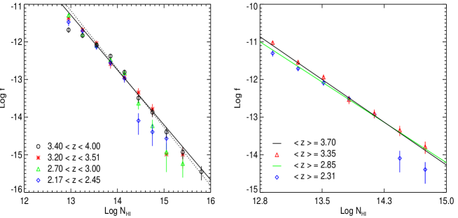
Kim et al.’s 1997 [9] analysis of the differential density distribution function (DDF) by redshift interval clearly shows an evolution in the departure from the power-law fit (Figure 2). In the left-hand panel of Figure 2 the $\langle z\rangle=3.70$ data [12] show only a slight steepening (dotted line) at the higher column densities, but by $\langle z\rangle=3.35$ a deficiency in the number density of clouds at $N_{\rm HI}>10^{14.8}~{}{\rm cm}^{-2}$ can be seen, while clouds at $\langle z\rangle=2.85$ and $\langle z\rangle=2.31$ show deviations from the power-law extrapolation at $N_{\rm HI}>10^{14.3}~{}{\rm cm}^{-2}$. This departure from a power law can be easily seen in the right-hand panel of Figure 2, where the distribution functions of the $\langle z\rangle=2.31$ (diamonds) and $\langle z\rangle=3.35$ (triangles) absorbers, now corrected for incompleteness, are shown. There are no clouds with $N_{\rm HI}>10^{15.2}~{}{\rm cm}^{-2}$ at $\langle z\rangle=2.31$ despite the fact that the redshift path is 1.5 times larger than at $\langle z\rangle=3.35$, so the deficiency of high column density clouds in the lower redshift range is not due to observational selection. We conclude that we are seeing a rapid evolution with redshift in the number density of absorbers at high column density, with the break in the density distribution function strengthening and migrating to lower column densities as redshift decreases.

Figure 3: $N(z)$ vs. redshift for the present data (filled circles) and the HST observations (open squares; open diamonds). The solid line shows the maximum likelihood fit to the HST data and the high column density Keck data (slope $\gamma=2.15$). The dotted line shows the fit to the Keck data only, with a slope of $\gamma=2.78$. Triangles show the forest clouds over just the column density range $N_{\rm HI}=10^{13.1}-10^{14}\ {\rm cm}^{-2}$, with a long dashed line fit with $\gamma=1.19$. The $1\sigma$ error bars and redshift binning are indicated for each point.

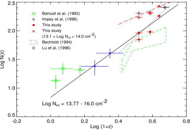
Turning to the number density evolution of Ly$\alpha$ clouds with redshift, where the number density of clouds per unit redshift per line of sight is expressed as: $N(z)=N_{0}(1+z)^{\gamma}$, we can compare the Keck data on the high redshift systems with the low redshift systems studied with HST [1],[8], while keeping in mind that $N(z)$ will be sensitive to the adopted threshold $N_{\rm HI}$ (a reflection of the departure from the single power-law description at $N_{\rm HI}>10^{14.3}~{}{\rm cm}^{-2}$). Figure 3 shows a plot of log$\,N(z)$ vs. log$\,(1+z)$ giving the maximum likelihood fit to the HST data and the high column density Keck data ($\gamma=2.15$). The adopted column density range used for the fit, $N_{\rm HI}=10^{13.77}-10^{16.0}~{}{\rm cm}^{-2}$, corresponds approximately to the conventional equivalent width threshold of $W=0.32$ Å for comparisons with the lower redshift data [1],[8],[2]. By contrast, the best fit to the slope of $N(z)$ for the low column density systems in the Keck data is $\gamma=1.19$. The definition of $N(z)$ yields $\gamma=1$ for $q_{0}=0$ and $\gamma=0.5$ for $q_{0}=0.5$ in the case of non-evolving clouds, and the slopes for the data in different column density ranges in Figure 3 can be understood in terms of the evolution of the break in the DDF: the number density of the higher column density systems ($\gamma=2.15$) is evolving rapidly, while the number density of the lower column density systems ($10^{13.1}<N_{\rm HI}<10^{14.0}~{}{\rm cm}^{-2}$; $\gamma=1.19$) is not.

3 The Evolution of b-Values

A second interesting issue is the evolution of line-widths, characterized by the Doppler parameter $b$ obtained from profile fitting, whose behavior reflects the thermal/ionization history of the IGM [5]. Hu et al.  1995 [6] found a typical mean $b$ of 28 km s^-1 with a minimal $b_{c}$ = 20 km s^-1 from the analysis of $\langle z\rangle=2.85$ systems. At $\langle z\rangle=3.70$ Lu et al.  [12] report a mean $b$ of 23 km s^-1 and cutoff $b_{c}$ = 15 km s^-1, showing a trend to narrower absorbing components at higher redshift.

In order to quantify these descriptions, it is important to run model simulations to understand the nature of blending, selection, and incompleteness effects on the analysis of the observed data. The procedure used [6],[12] is to input a truncated Gaussian distribution for the Doppler parameter values, generate a series of simulated artifical spectra, and then apply the standard profile-fitting methods to match the recovered column densities and $b$ values to the input spectra and to the observations.

Figure 4: Observed (dotted histogram) and simulated (solid histogram) $b$ distributions. For the $\langle z\rangle=3.35$ clouds, the low cut-off $b$ value is $\sim 17~{}{\rm km\ s}^{-1}$. For the $\langle z\rangle=2.31$ clouds, there is no single best-fit assumed distribution for $b$. Assuming that most narrow lines are unidentified metal lines towards Q1700+643 and ignoring the lines with $b<22~{}{\rm km\ s}^{-1}$, the cut-off $b$ of $24~{}{\rm km\ s}^{-1}$ which is shown in the figure best fits the data.

Both the cutoff and median $b$ values appear to increase with decreasing redshift — the cutoff $b$ value’s increase from 15 km s^-1 at $\langle z\rangle=3.70$, to $17~{}{\rm km\ s}^{-1}$ at $\langle z\rangle=3.35$, to $22~{}{\rm km\ s}^{-1}$ at $\langle z\rangle=2.85$, to $24~{}{\rm km\ s}^{-1}$ at $\langle z\rangle=2.3$ presumably reflecting an increase in the turbulent and thermal broadening over this period.

4 Summary

In broad outline the cloud evolution described here probably follows naturally from the decreasing IGM density with decreasing redshift, which drives down the column density at which shocking occurs [13], and the increasing level of structure which results in more turbulent components. However, reproducing the results in detail will require full comparison with a wide suite of numerical models, which may provide useful constraints on the history of the ionization and heating of the IGM.

Acknowledgements.  This work was partly supported by NSF grant AST 96-17216, and used observations obtained with Steve Vogt’s HIRES spectrograph for the Keck I telescope. The W. M. Keck Observatory is operated as a scientific partnership between the California Institute of Technology, the University of California, and the National Aeronautics and Space Administration.

References

- [1] Bahcall, J. N., et al. 1993, ApJS 87, 1
- [2] Bechtold, J. 1994, ApJS 91, 1
- [3] Bi, H. & Davidsen, A. F. 1997, ApJ 479, 528
- [4] Davé, R., Hernquist, L., Weinberg, D. H., & Katz, N. 1997, ApJ 477, 21
- [5] Haehnelt, M. G. & Steinmetz, M. 1997, MNRAS submitted [astro-ph/9706296]
- [6] Hu, E. M., Kim, T.-S., Cowie, L. L., Songaila, A., & Rauch, M. 1995, AJ 110, 1526
- [7] Hui, L., Gnedin, N. Y., & Zhang, Y. 1997, ApJ 486, 599
- [8] Impey, C. D., Petry, C. E., Malkan, M. A., & Webb, W. 1996, ApJ 463, 473
- [9] Kim, T.-S., Hu, E. M., Cowie, L. L., & Songaila, A. 1997, AJ 114, 1
- [10] Kim, T.-S., Hu, E. M., Cowie, L. L., & Songaila, A. 1997, these proceedings
- [11] Kirkman, D. & Tytler, D. 1997, ApJ 484, 672
- [12] Lu, L., Sargent, W. L. W., Womble, D. S., & Takada-Hidai, M. 1996, ApJ 472, 509
- [13] Mücket, J. P., Petitjean, P., & Riediger, R. 1997, A&A submitted
- [14] Petitjean, P., Webb, J. K., Rauch, M., Carswell, R. F., & Lanzetta, K. M. 1993, MNRAS 262, 499
- [15] Zhang, Y., Anninos, P., & Norman, M. L. 1995, ApJ 453, L57
- [16] Zhang, Y., Anninos, P., Norman, M. L., & Meiksin, A. 1997, ApJ 485, 496