Geomagnetic Field and Air Shower Simulations.

Abstract

The influence of the geomagnetic field on the development of air showers is studied. The well known International Geomagnetic Reference Field was included in the AIRES air shower simulation program as an auxiliary tool to allow calculating very accurate estimations of the geomagnetic field given the geographic coordinates, altitude above sea level and date of a given event. Some test simulations made for representative cases indicate that some quantities like the lateral distribution of muons experiment significant modifications when the geomagnetic field is taken into account.

1 Introduction

The charged particles of an air shower interact with the Earth’s magnetic field. One of the effects of such interaction is that of curving the particles’ paths.

In order to take into account such effect, we have incorporated the geomagnetic field (GF) in the AIRES air shower simulation program [1, 2] allowing to simulate the showers in presence of the field at any location and time.

We have first studied the principal characteristics of the GF: Its origin, magnitude and variations. Thereafter we have analyzed the different GF models that are normally used: The dipolar models [3] which as their name suggest, consider the GF as generated by magnetic dipoles whose magnitude and orientation are set to fit the experimental measurements; the so-called International Geomagnetic Reference Field (IGRF) [4], a more elaborated model, based on a high-order harmonic expansion whose coefficients are fitted with data coming from a network of geomagnetic observatories all around the world.

In this paper we present a simple comparative analysis of the different models. One of the conclusions that comes out from our analysis is that the dipolar models are not useful to evaluate the GF at a given arbitrary location with enough accuracy, a more sophisticated model like a high order series expansion is needed instead. On the other hand, the predictions of the IGRF proved to match with the corresponding experimental data with errors that are at most a few percent.

We have therefore selected the IGRF to link it to the simulation program AIRES, as an adequate model to synthesize the GF at a given geographical location and time.

This work is organized as follows. In section 2 we start describing the GF. In sections 3 and 4 we mention some of the different models of the GF that exist at present. We analyze them and in section 5 we compare the predictions of these models with the experimental data.

The practical implementation of the GF in the AIRES program is discussed in section 6. Section 7 is devoted to the analysis of the effects of the GF on some air shower observables, and in section 8 we place our final remarks and conclusions.

2 Description of the geomagnetic field

The Earth’s magnetic field is normally described by seven parameters, namely, declination (D), inclination (I), horizontal intensity (H), vertical intensity (Z), total intensity (F) and the north (X) and east (Y) components of the horizontal intensity. D is the angle between the horizontal component of the magnetic field and the direction of the geographical north and I is the angle between the horizontal plane and the total magnetic field. It is considered positive when the magnetic field points downwards. Also Z is positive when I is positive [3].

The geomagnetic poles are located, by definition, in the places where the field lines are perpendicular to the Earth’s surface. The physical locations of the magnetic poles are actually areas rather than single points. Because of the changing nature of the GF, the locations of the magnetic poles also change. The current location of the N (S) magnetic pole is approximately $78.5^{\circ}$ N and $103.4^{\circ}$ W ($65^{\circ}$ S and $139^{\circ}$ W).

The GF is generated by internal and external sources. The first ones are related to processes in the interior of the Earth’s core while the external sources would be related to ionized currents in the high atmosphere [3]. The experimental measurements show that the internal field is significantly greater than the external contribution. The former goes from 20.000 to 70.000 nanoteslas (nT, 1 nT = $10^{4}$ gauss) while the external contribution is around 100 nT.

The GF evolves with time. The rates of change of the different components are not uniform over position and time and can be classified as follows [3]:

• Secular variations: Extended over years with generally smooth increases or decreases in the field. They are originated by the internal field and are the least understood of all the kinds of changes that affect the GF. The values of the secular variation of the components of the GF go from 10 nT per year up to 150 nT/year and up to 6 to 10 arc minutes/year for D and I.

• Periodic variations: They are originated by the external field and in general amount to less than 100 nT. The characteristic periods are 12 hs, 1 day, 27 days, 6 months and 1 year. They are related with the Earth’s rotation and with the Solar and Lunar influence.

• Magnetic storms: Sudden disturbances in the GF which may last from hours up to several days and rarely modify the field in more than 500 nT.

3 Models of the geomagnetic field

3.1 Dipolar model

The simplest way to model the GF is to assume that it is generated by a magnetic dipole. Two alternative dipolar models are normally taken into account [3]:

• Dipolar central model: It is assumed that the field is generated by a dipole with origin in the center of the Earth, inclined some degrees with respect of the rotation axis. This model is used to define the geomagnetic coordinates (they are the coordinates from the dipole’s axis): a) Geomagnetic latitude, $\varphi^{*}$, measured from the geomagnetic equator, defined as the plane normal to the dipole’s axis and passing through the center of the Earth, b) Geomagnetic longitude, $\lambda^{*}$, measured eastwards from the meridian half-plane containing the geographical south pole.

  The geomagnetic coordinates $(\varphi^{*},\lambda^{*})$ of each point P have a one-to-one relationship with the point’s geographical coordinates $(\varphi,\lambda)$. The transformation formulae can be deduced using spherical trigonometry or rotation matrices.

• Dipolar eccentric model: The field is generated by a dipole displaced from the center of the Earth.

3.2 Harmonic analysis of the geomagnetic field

When a more accurate reproduction of the field is needed, it is necessary to go beyond the dipole approximation and make a higher order harmonic analysis of the GF [3]: The GF is modeled like the magnetostatic field whose sources are currents located in the interior of the Earth. Then for points located near the Earth’s surface, it is possible to calculate the GF using the scalar magnetic potential $\phi$, via $\mathbf{B}=-\mathop{\mathbf{g}rad}\nolimits\phi$. Such scalar potential satisfies Laplace’s equation, $\nabla^{2}\phi=0$.

Due to the spherical symmetry of the problem, the solution can be conveniently expressed in terms of Legendre functions. The scalar magnetic field can be expanded in terms of the geographical coordinates as

$$\phi=a\mathop{\displaystyle\sum}\limits_{n=1}^{N}\mathop{\displaystyle\sum}\limits_{m=0}^{n}\QOVERD(){a}{r}^{n+1}\left[g_{nm}\cos m\lambda+h_{nm}\sin m\lambda\right]P_{n}^{m}(\cos\varphi)$$ (1)

where $a$ is the mean radius of the Earth (6371.2 km), $r$ is the radial distance from the center of the Earth, $\lambda$ is the longitude eastwards from Greenwich, $\varphi$ is the geocentric colatitude, and $P_{n}^{m}(\cos\varphi)$ is the associated Legendre function of degree $n$ and order $m$, normalized according to the convection of Schmidt. $N$ is the maximum spherical harmonic degree of the expansion.

4 International Geomagnetic Reference Field

The International Geomagnetic Reference Field (IGRF) [4] is a parameterization of experimental values using equation (1). Sets of spherical harmonic coefficients ($g_{nm}$ and $h_{nm})$ at 5-year intervals starting from 1900 are evaluated. They are determined from the measurements of the components of the field made at the Earth’s surface (geomagnetic observatories and satellite observations). Coefficients for dates between 5-year epochs are obtained by linear interpolation between the corresponding coefficients for the neighboring epochs. At present, the model includes secular variation terms for forward continuation of it for the years 1995 to 2000.

The error of the field components and the D and I angles are respectively less than 500 nT and 30 arc minutes. These errors are relatively small (for example they amount to a few percent in the case of the field intensity F) and this makes the IGRF model a very useful tool to estimate the GF at any geographic location and any time belonging to its validity interval.

5 Analysis of the different models

We have evaluated the results coming from the models already introduced in a variety of situations, in order to establish which of them is the most convenient to cover the needs arising in an air shower simulation algorithm.

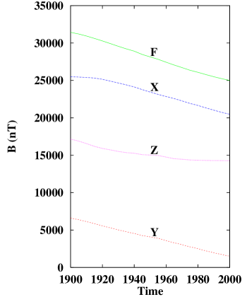
Figure 1: Secular variation of the GF (1900-2000). Site: El Nihuil (Argentina).

To start with, we have used the IGRF series expansion to study the secular variation of the GF at a fixed site, namely the El Nihuil site (lat. $35.2^{\circ}$ S, long. $69.2^{\circ}$ W, altitude 1400 m.a.s.l.) located in Argentina. In figure 1 the components of the GF are displayed as functions of time for the years 1900-2000. The rate of change of the field intensity F is roughly 20 %/century. The variation of the field components with time must therefore be taken into account if it is necessary to reproduce the GF within a few percent error limit.

We have also studied the spatial variation of the GF at a given fixed time. In figure 2 the components of the GF are plotted versus the geographic latitude for the fixed longitude of $69^{\circ}$ W (longitude of the El Nihuil site). There are two main conclusions that can be extracted from these plots: (1) The spatial variations of the field components are very important: Notice, for example, that the field intensity, F, goes from a minimum of 24000 nT up to 58000 nT, that is, more than twice the minimum value, (2) The predictions of the dipole models, either centered or eccentric, can differ in more than 30 % with respect to the IGRF and hence with experimental values. Therefore these models cannot be used to produce safe estimations of the GF at any given arbitrary location.

$$\begin{array}[]{cc}\hbox{\psfig{width=199.16928pt}}&\hbox{\psfig{width=199.16928pt}}\\ \hbox{\psfig{width=199.16928pt}}&\hbox{\psfig{width=199.16928pt}}\end{array}$$

Figure 2: Comparison of different GF models (dipolar centered and eccentric, and IGRF models).The Cartesian components of the GF are plotted versus geographic latitude (fixed longitude: $69^{\circ}$ W).

The facts presented so far allow to establish the IGRF as the most convenient model that can give accurate estimations of the GF to be used in air-shower simulations. As a final test, we have checked the IGRF predictions against experimental data [5].

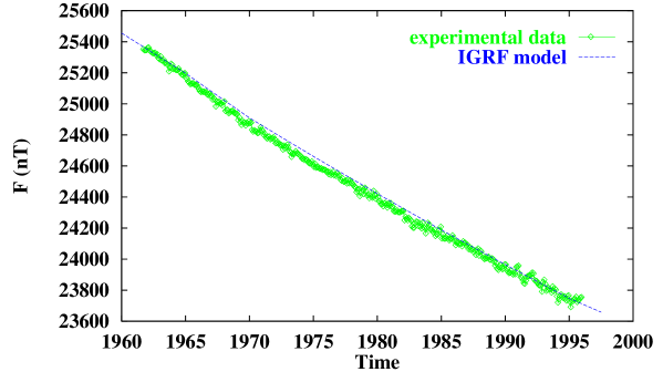
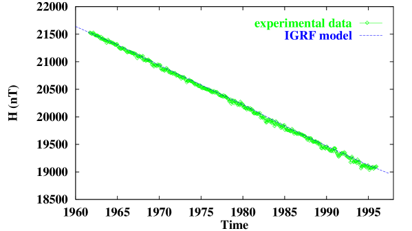
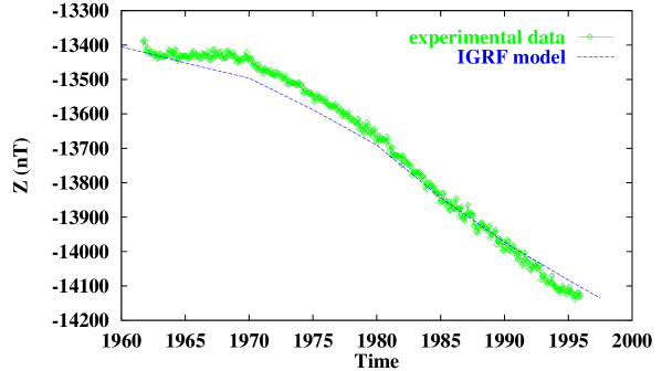
Figure 3: Comparison between experimental data and the IGRF model. The absolute difference between the experimental and the IGRF prediction is always less than 200 nT.(Experimental data: Las Acacias observatory, Argentina [5]).

In figure 3 the F, H and Z components are plotted against time. The absolute difference between estimated and measured fields is always less than 200 nT which is below the 500 nT error bound previously mentioned.

The accuracy of the IGRF predictions is also maintained during magnetic storms. In figure 4 we illustrate this fact. The experimental data were registered at the Trelew observatory in Argentina and corresponds to a magnetic storm that took place during 1994. Again we can see that the 500 nT bound is always larger than the actual errors. The analysis of the errors in the declination and inclination angles (not displayed here) indicates that such errors are always less than 0.5 degree.

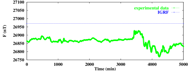
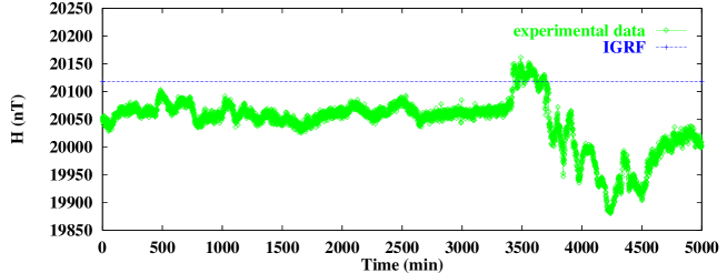
Figure 4: Magnetic storm: Experimental data and IGRF model. The difference between the experimental and the IGRF prediction is always less than 500 nT. (Experimental data: Trelew observatory, Argentina [5]).

6 Practical Implementation

The calculation of the GF in any place and time as well as the dynamics of charged particles in such field have been incorporated into the AIRES program [2].

6.1 Calculation of the GF in the AIRES program

Special subroutines using the IGRF model for the calculation of the geomagnetic field have been incorporated to the AIRES program [2, 4].

The GF calculations are controlled from the input instructions. By means of suitable IDL directives [1, 2] the user can either specify a date and the geographic coordinates of a site to allow automatic IGRF calculations, or enter manually the GF components (intensity, inclination and declination).

It is assumed that the shower develops under the influence of a constant and homogeneous magnetic field which is evaluated before starting the simulations. Since the region where the shower develops is very small when compared with the Earth’s volume, the mentioned approximation of a constant and homogeneous field is amply justified.

6.2 Dynamics of charged particles

Let us consider the motion of a particle with charge $q$ in a uniform, static magnetic field $\mathbf{B}$ . The equations of motion are (MKS units):

$$\frac{d\mathbf{p}}{dt}=q\ \mathbf{v}\times\mathbf{B}$$ (2)

where $q,$ $\mathbf{v,}$ and $\mathbf{p}$ are the particle’s charge, velocity and linear momentum respectively.

Since the particle’s energy is constant in time, the magnitude of its velocity is constant and so the Lorentz factor, $\gamma$. The equation of the unit velocity vector, $\widehat{\mathbf{u}}=\frac{\mathbf{v}}{\shortmid\mathbf{v\shortmid}}$, can then be written

$$\frac{d\widehat{\mathbf{u}}}{dt}=\QOVERD(){qc^{2}}{E}\widehat{\mathbf{u}}\times\mathbf{B}$$ (3)

where $E$ is the total energy of the particle (rest plus kinetic) and $c$ is the speed of light.

As it is well known, the trajectory of a charged particle interacting with a uniform magnetic field is an helix whose axis is parallel to $\mathbf{B.}$ The motion in a plane normal to the magnetic field is circular, with angular velocity

$$\omega=\frac{qc^{2}B}{E}.$$ (4)

If the particle advances a distance $\Delta s$ in a time $\Delta t$ ($\Delta s=\beta c\Delta t$, $\beta=v/c$), the motion can be approximately calculated via:

$$\widehat{\mathbf{u}}(t+\Delta t)\cong\widehat{\mathbf{u}}(t)+\frac{d\widehat{\mathbf{u}}}{dt}\Delta t=\widehat{\mathbf{u}}(t)+\QOVERD(){qc^{2}\Delta t}{E}\widehat{\mathbf{u}}\times\mathbf{B}.$$ (5)

For this approximation to be valid, it is needed that

$$\omega\Delta t=\frac{\omega\Delta s}{\beta}\ll 1.$$ (6)

We have studied the deflection of particles in various representative cases finding that equation (6) is always satisfied for all the particles that are tracked during the simulation of air-showers, even in the least favorable case of low energy electrons or positrons. It is therefore safe to use equation (5) to account for the deflections of charged particles moving under the effect of the GF.

The magnetic deflection algorithm implemented in AIRES makes use of equation (5) to evaluate the updated direction of motion at time $t+\Delta t$. However, it also uses a “technical trick”, inspired in a similar procedure used in the well-known program MOCCA [6]: The path $\Delta s$ is divided in two halves of length $\Delta s/2$ each. Then the particle is moved the first half using the old direction of motion $\widehat{\mathbf{u}}(t)$, and the second one with the updated vector $\widehat{\mathbf{u}}(t+\Delta t).$ This means that the correction at time $\Delta t$ is applied starting at $t=\Delta t/2$ and, as a result, compensates for the inaccurate direction $\widehat{\mathbf{u}}(t)$ used in the first half.

Figure 5: Schematic representation illustrating the algorithm used in AIRES to move charged particles under the influence of the GF. The complete path is divided in two halves each one of length $\Delta s/2$. The particle is advanced the first half using the current direction of motion. The direction of motion is updated to its final value and finally the particle is advanced the second half using this new direction. In this figure the radius of curvature was exaggeratedly reduced to 10 cm in order to make visible the difference between exact and calculated paths. For realistic conditions such differences are completely negligible.

In figure 5 the advancing-deflecting procedure is represented schematically. Here the radius of curvature of the exact trajectory was deliberately reduced to make evident the differences between the exact and approximate paths. In the case of realistic curvature radii (of hundreds or thousands of meters) both exact and simulated trajectories are virtually coincident.

7 Simulations

We have analyzed the influence of the GF on air shower observables performing some simulations in a variety of initial conditions.

We have simulated 10¹⁹ eV proton air showers with varying injection altitudes and zenith angles (from 0 to 80 deg), thinning levels range from 10^-4 to 10^-7 relative. We have chosen the Millard county (Utah, USA) site where the GF is intense and therefore the differences between the simulations with and without field can be appreciated better.

The direct inspection of global observables such as shower maximum, total number of particles at ground, etc. shows no evident effect of the GF. Some tendencies can be detected when a large number of showers is simulated, and in most cases the deviations are of the order of the fluctuations, either natural or induced by thinning.

However, differences do appear when a detailed analysis of some particle distributions is made. To illustrate this point we are going to report here the results of some of our simulations.

All the selected showers were simulated at 10^-7 relative thinning level in order to obtain clear data; the magnetic field, when enabled, amounts to 52800 nT (F) with an inclination ${\mathrm{I}}=64.8$ degrees; the zenith angle is 70 degrees and the azimuth 90 degrees (incidence plane normal to the magnetic north). The ground level is located at 1000 m.a.s.l (920 g/cm²) and we have considered two injection altitudes case A: 9350 m ($X=300$ g/cm²) and case B: 100 km ($X\cong 0$).

The mean positions of the shower maximum are, approximately, 560 g/cm² (case A) and 280 g/cm² (case B). The path from the mean shower maximum down to the ground level, measured along the shower axis, for case A (B) is 1050 g/cm² (1870 g/cm²). As a result, the attenuation of the showers at ground level is larger for case B than for case A; and the number of particles reaching ground is thus much smaller for case B. For example, without the effect of the GF the total number of electrons and positrons reaching ground for case A is $(1.6\pm 0.4)\times 10^{8}$, while the figure corresponding to case B is $(4.7\pm 0.5)\times 10^{6}$, that is 34 times smaller than the previous case.

The reason for selecting these two cases was to investigate the influence of the GF in two different phases of the shower development: (A) shortly after reaching its maximum and (B) when the shower is about to vanish completely.

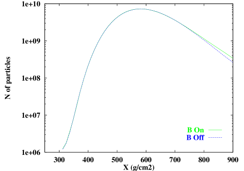
Figure 6: Longitudinal development of all charged particles (case A).

Let us start our comparative analysis studying the longitudinal development of all charged particles. In figure 6, the total number of charged particles is plotted against the vertical depth $X$. The initial conditions are the ones corresponding to the case A. Comparing the plots coming from the simulations with and without GF we can see that there is no significant difference either in the position of the maximum ($X_{\mathrm{m}ax}$) or in the maximum number of charged particles ($N_{\mathrm{m}ax}$). Even if the showers simulated without GF seem to vanish more quickly as $X$ grows, this difference may not be significant since it is never larger than one standard deviation of the corresponding mean.

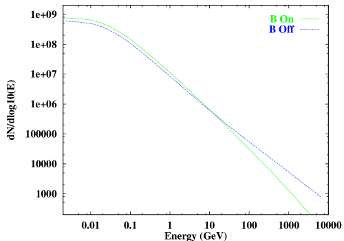
Figure 7: $\gamma$ ground energy distribution (case A).

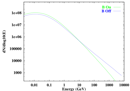
Figure 8: $e^{+}$ and $e^{-}$ ground energy distribution (case A).

The ground level energy distributions of $\gamma$’s and $e^{\pm}$’s (case A) are plotted in figures 7 and 8 respectively. When the GF is enabled both ground energy distributions change in the same way: In both cases the number of particles that reach the ground increases for low energy particles and decreases for high energy ones. The correlations between the respective distributions can be understood taking into account that ground electrons, positrons or gammas surely come from the “nearby” electromagnetic cascade whose intrinsic mechanisms constantly generate gammas from $e^{\pm}$ and vice-versa, being the energies of the secondaries lower (at most equal) than those of the respective primaries. It is therefore clear that the structure of both energy distributions should be similar. When the GF is considered, the trajectory of electrons and positrons are helicoidal. This generally leads to an increase of the particles’s paths and therefore to larger continuum energy losses (ionization losses), diminishing (enlarging) the average number of high (low) energy particles that reach ground.

The ground $\mu^{\pm}$ energy distributions (case A) are plotted in figure 9. There are no measurable differences between the energy distributions corresponding to the cases with and without GF for these particles. The muons travel long distances without interacting and their radii of curvature are generally larger than for $e^{\pm}.$ This implies that these particles reach the ground without important increases in their paths and thus without modifications in their energy.

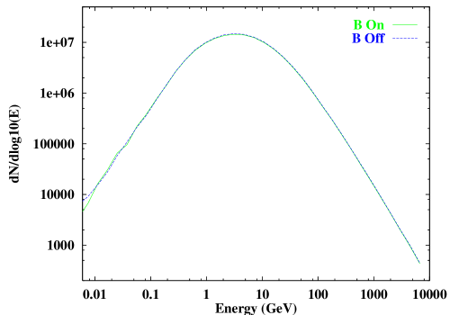
Figure 9: $\mu^{+}$ and $\mu^{-}$ ground energy distribution (case A).

On the other hand, the lateral distribution of ground muons does present significant modifications when the GF is considered.

To evaluate the densities plotted in figures 10 (case A) and 11 (case B) we have filtered all the muons arriving at ground at points $(x_{g},y_{g})$ verifying $\left|\arctan\frac{y_{g}}{x_{g}}\right|<10^{\circ}$. In other words, we have selected particles lying in the region close to the $x$-axis (in polar coordinates, no more than 10 degrees apart) where the effects of the magnetic deflection are most noticeable. To make the corresponding histograms, both the positive and negative $x$-axis were divided in radial bins $[r_{i},r_{i+1}]$, with $r_{1\ldots 8}=150$, 200, 300, 400, 600, 800, 1200 and 1600 meters.

The symmetry of distributions around the origin when the GF is disabled shows up clearly in figures 10 and 11 where the $\mu^{+}$ and $\mu^{-}$ distributions (${\mathbf{B}}$ off) are virtually coincident.

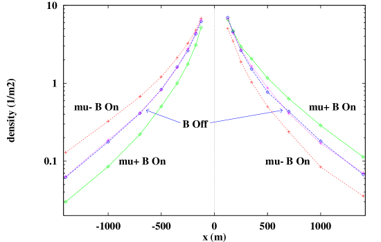
Figure 10: Density of $\mu^{+}$ and $\mu^{-}$ for particles arriving near the $x$-axis, case A (see text).

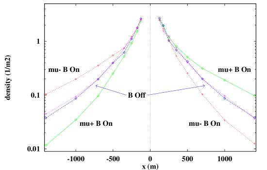
Figure 11: Same as figure 10, but for case B.

On the other hand, when the GF is on, a displacement of the density of positive (negative) particles towards positive (negative) $x$-axis occurs. Fitting the simulation data to suitable distribution functions with the central position as a free parameter, it is possible to estimate the difference between the peaks in the $\mu^{+}$, $\mu^{-}$ distributions in about 70 m.

The difference between the numbers of $\mu^{+}$ and $\mu^{-}$ increases with the distance to the shower core arriving to about one order of magnitude at $|x|=2000$ m for the case of completely developed showers (figure 11). Notice also that the total number of muons ($\mu^{+}$ and $\mu^{-}$) also changes when the GF is switched on.

Another way of studying the influence of the GF on the muon distribution is to analyze the dependence of the ground particle density $\rho(r,\theta)$ with the polar angle $\theta$, for $r$ belonging to a certain interval $[r_{1},r_{2}].$

The $\mu^{\pm}$ densities versus polar angle $\theta$ are plotted in figures 12 (case A) and 13 (case B), for $[r_{1},r_{2}]=[100\>{\mathrm{m}},200\>{\mathrm{m}}]$ and [300 m, 600 m] .

$$\begin{array}[]{cc}\hbox{\psfig{width=206.28247pt}}&\hbox{\psfig{width=206.28247pt}}\\ \hbox{\psfig{width=206.28247pt}}&\hbox{\psfig{width=206.28247pt}}\end{array}$$

Figure 12: Density of $\mu^{+}$ and $\mu^{-}$ at ground $\rho(r,\theta)$ versus polar angle $\theta$ for $100\leq r\leq 200$ m and $300\leq r\leq 600$ m (case A).

$$\begin{array}[]{cc}\hbox{\psfig{width=206.28247pt}}&\hbox{\psfig{width=206.28247pt}}\\ \hbox{\psfig{width=206.28247pt}}&\hbox{\psfig{width=206.28247pt}}\end{array}$$

Figure 13: Same as figure 12, but for case B.

When the GF is off, the plotted data show the anisotropy due to the nonzero zenith angle of the shower axis. Notice that all the densities reach their maximum in the zone that is closest to the arrival direction ($\theta\cong 90$ deg).

The plots corresponding to the simulations with the GF enabled are consistent with the data displayed in figures 10 and 11: The $\mu^{+}$ ($\mu^{-})$ distribution is larger in the positive (negative) $x$-axis region, $\theta\cong 0^{\circ}$ ($\theta\cong 180^{\circ}$).

Such characteristics show up clearly in the plots corresponding to the [300 m, 600 m] zone. For the [100 m, 200 m] zone the approximately unaltered number of $\mu^{+}$ ($\mu^{-})$ in the proximity of $\theta=0^{\circ}$ ($\theta=180^{\circ}$) is due to the fact that the zone is located too much near the peak of the distribution (See figure 10).

In the case of electrons and positrons, the fluctuations are large enough to prevent the detection of any relevant difference in particle distributions. This clearly shows up in figure 14 where the $e^{\pm}$ densities (case A) were plotted in similar conditions as in the $\mu^{\pm}$ case.

$$\begin{array}[]{cc}\hbox{\psfig{width=206.28247pt}}&\hbox{\psfig{width=206.28247pt}}\\ \hbox{\psfig{width=206.28247pt}}&\hbox{\psfig{width=206.28247pt}}\end{array}$$

Figure 14: Same as figure 12, but for $e^{+}$ and $e^{-}$ densities (case A).

8 Conclusions

We have discussed in this work the influence of the geomagnetic field on the most common observables that characterize the air showers initiated by astroparticles. The data used in our analysis were obtained from computer simulations performed with the AIRES program.

Our work includes the analysis of the main properties of the geomagnetic field, as well as the implementation of the related algorithms in the program AIRES.

By means of the International Geomagnetic Reference Field (IGRF) it is possible to make accurate evaluations of the average geomagnetic field at a certain place given its geographical coordinates, altitude above sea level and time.

We have used this tool to run the simulations using a realistic geomagnetic field, selecting the location of Millard county (Utah, USA) as a convenient place with a high magnetic field intensity.

The changes that the analyzed magnitudes experiment when the geomagnetic field is taken into account are generally small, but there are certain observables like the lateral distribution of muons where such differences become significant.

Considering these facts we conclude saying that the geomagnetic field should be taken into account whenever a particular event with precisely determined initial conditions must be simulated accurately.

In future works we will address another effects on the air shower development that are related to the geomagnetic field.

References

- [1] S. J. Sciutto, AIRES: A minimum document, Pierre Auger Observatory technical note GAP-97-029 (1997).
- [2] S. J. Sciutto, AIRES, a system for air shower simulations. User’s manual and reference guide, in preparation.
- [3] Chapman, S., and J. Bartels, Geomagnetism, Oxford Univ.Press (Clarendon), London and New York, Volumes 1 and 2, 1940.
- [4] The data, software and documentation related with the International Geomagnetic Reference Field are distributed by the National Geophysical Data Center, Boulder (CO), USA, and can be obtained electronically at the following Web address: www.ngdc.noaa.gov.
- [5] J. Gianibelli, Center of Geomagnetic Studies, La Plata University, private communication.
- [6] A. M. Hillas, Proc. 19th ICRC (La Jolla), 1, 155 (1985).