THE X–RAY BACKGROUND AND THE ROSAT DEEP SURVEYS

In this article we review the measurements and understanding of the X-ray background (XRB), discovered by Giacconi and collaborators 35 years ago. We start from the early history and the debate whether the XRB is due to a single, homogeneous physical process or to the summed emission of discrete sources, which was finally settled by COBE and ROSAT. We then describe in detail the progress from ROSAT deep surveys and optical identifications of the faint X-ray source population. In particular we discuss the role of active galactic nuclei (AGNs) as dominant contributors for the XRB, and argue that so far there is no need to postulate a hypothesized new population of X-ray sources. The recent advances in the understanding of X-ray spectra of AGN is reviewed and a population synthesis model, based on the unified AGN schemes, is presented. This model is so far the most promising to explain all observational constraints. Future sensitive X-ray surveys in the harder X-ray band will be able to unambiguously test this picture.

1 Introduction

It is a heavy responsibility for us, as it would be for everybody else, to write a paper on the X–ray Deep Surveys and the X–ray background (XRB) for this book, in honour of Riccardo Giacconi. Everybody recognizes the importance of Riccardo’s contribution in both these fields. The discovery of the XRB using proportional counters in a rocket flight, the UHURU satellite, the first X–ray telescope with focusing optics “Einstein” are milestones in X–ray astronomy and Riccardo played a leading role in these experiments. More recently he gave a fundamental contribution to the planning, execution and analysis of the ROSAT Deep Surveys. As a consequence of this, a significant fraction of the results which we will describe in this paper either are his own results or are based on experiments which he conceived and led to success.

In Section 2 we give a brief historical overview of the XRB problem, from its discovery up to the results obtained in the eighties with the HEAO–1 and Einstein missions. During these years the origin of the XRB has been discussed mainly in terms of two alternative interpretations: the diffuse hypothesis (e.g. hot intergalactic gas) and the discrete source hypothesis. The existence of these radically alternative hypotheses has not been “neutral” with respect to devising experiments which wanted to study the XRB. In fact, if the XRB were mainly due to discrete sources, experiments aimed at studying the single sources responsible for it would obviously need high angular resolution in order to detect and resolve the large number of expected faint sources. Vice versa, if the XRB were mainly diffuse, source confusion would not be a problem and one could safely abandon the high angular resolution option. In this case the crucial experiment would be a measurement as accurate as possible of the spectrum in order to reveal the dominant physical production processes. The two working hypotheses led various groups of scientists to design very different sets of experiments $\!{}^{{\bf?}}$. In Section 3 we present and discuss some recent results from deep surveys with ROSAT. These surveys have already resolved into discrete sources $\sim$ 70% of the measured XRB in the 1–2 keV band. The available optical identifications, still in progress, suggest that AGNs are the dominant population at these faint X–ray fluxes. Finally, in Section 4 we discuss some models which, taking into account the existing observational data on AGNs, are able to produce reasonably good fits to the XRB spectrum up to $\sim$ 100 keV. The discussion is summarized in section 5.

2 The Early History of the X–ray Background

The existence of a diffuse XRB was discovered more than 35 years ago $\!{}^{{\bf?}}$. The aim of the experiment was to measure the X–ray emission from the Moon, but the data showed something unexpected: a strong X–ray source about 30 degrees away from the Moon (Sco X–1) and a diffuse emission approximately constant from all the directions observed during the flight. After this discovery, the first real improvement in our knowledge of the XRB has been made with the first all–sky surveys (UHURU and ARIEL V) at the beginning of the seventies. The high degree of isotropy revealed by these surveys led immediately to realize that the origin of the XRB has to be mainly extragalactic. Moreover, under the discrete source hypothesis, the number of sources contributing to the XRB has to be very large $\!{}^{{\bf?}}$ ($N>10^{6}\,sr^{-1}$).

In the same years a number of experiments were set up to measure the spectrum of the XRB over a large range of energy. It was found that over the energy range 3–1000 keV the XRB spectrum is reasonably well fit with two power laws with energy indices $\alpha_{1}\sim 0.4$ for $E\leq 25$ keV and $\alpha_{2}\sim 1.4$ for $E>25$ keV (see Figure 1 in $\!{}^{{\bf?}}$).

At the beginning of the eighties two different sets of measurements led additional fire to the debate between supporters of the discrete source and diffuse hypotheses. On the one hand, the excellent HEAO–1 data showed that in the energy range 3–50 keV the shape of the XRB is very well fit by an isothermal bremsstrahlung model corresponding to an optically thin, hot plasma with kT of the order of 40 keV $\!{}^{{\bf?}}$. Moreover, it was shown that essentially all Seyfert 1 galaxies with reliable 2–20 keV spectra ($\sim$ 30 objects, mostly from HEAO–1 data) were well fit by a single power law with an average spectral index of the order of 0.65, significantly different from the slope of the XRB in the same energy range $\!{}^{{\bf?}}$. Since Active Galactic Nuclei (AGNs) were already considered the most likely candidates for the production of the XRB under the discrete source hypothesis $\!{}^{{\bf?}}$, these two observational facts were taken as clear “evidence” in favour of the diffuse thermal hypothesis. On the other hand, the Einstein observations were suggesting a different scenario:

a) Pointed observations of previously known objects very soon showed that AGNs, as a class, are luminous X–ray emitters $\!{}^{{\bf?}}$.

b) When a larger AGN sample became available, it was confirmed that AGNs could contribute most of the diffuse soft XRB $\!{}^{{\bf?}}$. Actually, in order to avoid a contribution from AGNs larger than the observed background, it was concluded $\!{}^{{\bf?}}$ that the optical counts of AGNs had to flatten at magnitudes slightly fainter than the limit of the optically selected samples existing at that time. Such a flattening was later seen in deeper optical surveys.

c) Deep Einstein surveys showed that about 20% of the soft XRB (1–3 keV) is resolved into discrete sources $\!{}^{{\bf?},{\bf?},{\bf?},{\bf?}}$ at fluxes of the order of a few $\times\,10^{-14}erg\,cm^{-2}s^{-1}$. A large fraction of these faint X–ray sources were identified with AGNs.

Because of the difference between the spectra of the XRB and those of the few bright AGNs with good spectral data, the supporters of the diffuse, hot plasma hypothesis had to play down as much as possible the contribution of AGNs to the XRB to a limit which was close to be in conflict with an even mild extrapolation of the observed log(N)–log(S). Actually, a number of papers were published in which it was “demonstrated” that even in the soft X–ray band AGNs could not contribute much more than what had already been detected at the Einstein limit.

At that time we personally think that there was already evidence (for those who wanted to see it…) that the diffuse thermal emission as main contributor to the background was not tenable (see, for example, $\!{}^{{\bf?}}$). Very simple arguments in this direction were given in $\!{}^{{\bf?}}$. On the basis of reasonable extrapolations of the X–ray properties and the optical counts of known extragalactic X–ray sources (mainly AGNs and galaxies), Giacconi and Zamorani concluded that it is unlikely that their contribution to the soft X–ray background is smaller than 50%. Given this constraint, they then discussed two possibilities:

i) either faint AGNs have the so–called (at that time) “canonical” spectrum observed for brighter AGNs. In this case the residual XRB (i.e. the spectrum resulting after subtraction of the contribution from known sources) would not be fitted anymore by optically thin bremsstrahlung;

ii) or spectral evolution for AGNs is allowed. In this case, in order not to destroy the excellent thermal fit in the 3–50 keV data, diffuse emission could still be accommodated only if discrete sources have essentially the same spectrum as the XRB. On this basis, they concluded that “since in this scenario we would already require that the average spectrum of faint sources yielding 50% of the soft XRB is essentially the same as the observed XRB, there is nothing that prevents us from concluding that the entire background may well be due to the same class of discrete sources, at even fainter fluxes”.

In other words, reversing the usual line of thought, the excellent thermal fit of the 3–50 keV XRB spectrum was shown by these arguments to be a point in favour of the discrete source hypothesis, rather than of the hot gas hypothesis! These conclusions, however, were not well received in a large fraction of the X–ray community; probably, they had the defect of being too simple and direct…

Thus, the debate between the supporters of the two hypotheses continued, until the final resolution of the controversy came from the incredibly neat results obtained with the FIRAS instrument on board COBE: the absence of any detectable deviation from a pure black body of the cosmic microwave background set an upper limit to the comptonization parameter $y<10^{-3}$, more than ten times smaller than the value required by the hot intergalactic gas model $\!{}^{{\bf?}}$. The most recent upper limit for the comptonization parameter $\!{}^{{\bf?}}$ is now $y<2.5\times 10^{-5}$. Discussing these data, in $\!{}^{{\bf?}}$ it is concluded that a uniform, hot intergalactic gas produces at most $10^{-4}$ of the observed XRB!

3 The ROSAT Deep Surveys

3.1 Instrumental considerations

The detailed preparation for ROSAT Deep Survey observations started in 1984, well in advance of the actual ROSAT mission. At this time the engineering model of the ROSAT Proportional Counter PSPC $\!{}^{{\bf?}}$ had already been calibrated in the laboratory and the task was at hand to understand and try to correct for the various electronic and geometric distortions and gain non–linearities, which in general plague imaging proportional counters. Non–linearities in the performance of the Einstein IPC have e.g. set the final sensitivity threshold for Einstein Deep Surveys $\!{}^{{\bf?},{\bf?}}$. The ROSAT PSPC, even at the raw coordinate level, shows a higher degree of uniformity than the IPC. It was therefore possible to largely correct the significant distortions present in the PSPC data $\!{}^{{\bf?}}$. Figure 1 shows the comparison of a PSPC ground calibration flat field before and after correction of the distortion effects.

Figure 1: The ROSAT PSPC flat-field in detector coordinates. Left: uncorrected; right: corrected for geometric distortions (the web-like shadow is due to the mechanical support structure of the PSPC window).

These images immediately indicate another geometrical problem. While it is obviously possible to remove the distortions created by the detector itself, the shadows cast by the complicated wire-mesh in front of the PSPC cannot be corrected for. The mere fact that the 100$\mu$ wire shadow can be detected, demonstrates the relatively good angular resolution of the PSPC. In the early days we were still hoping that the satellite pointing instability would wash out any residual flat-field inhomogeneities.

Roughly at the same time we started prototyping the ROSAT scientific analysis software. Early ideas about local and map-detect algorithms, background estimation etc. were taken over from the Einstein analysis system. However, substantial improvements were incorporated, the most important of which was probably the rigorous application of Poisson statistics and maximum likelihood estimators in all statistical computations.

In order to test and understand the analysis algorithms we developed a science simulator system, which turned out to be one of our most powerful tools in the preparation of the science mission. During the course of time the simulation models became more and more realistic, including extended and point sources, time variability, different spectral models and realistic number counts for the X–ray sources as well as cosmic and solar scattering backgrounds. Orbital variation of the exposure time and background components due to the radiation belts were included as well. Every individual photon was traced through a realistic model of the X–ray mirror system and the detector $\!{}^{{\bf?}}$. Comparing input and output information, the detection algorithms could be tested, calibrated and, if necessary, improved.

In 1985 the first data about the performance of the ROSAT attitude control system became available from dynamical hardware-in-the-loop tests. It turned out that the attitude control was much more stable than specified and anticipated. Simulations including realistic attitude data indicated that sources in the center of the PSPC field could easily get lost behind shadows of the PSPC support grid. Less than a year from the originally planned launch (1987) we were able to convince the funding agency and industry to introduce a “wobble mode” into the attitude control system, which was to become the standard ROSAT pointing mode. Instead of wandering around at random, the spacecraft pointing direction is guided smoothly into a linear periodic zig-zag motion with a period of 402 seconds and an amplitude of $\pm 3$ arcmin ($\pm 1$ arcmin for the HRI) diagonal with respect to the detector coordinates. The wobble-mode, while introducing artificial periodic power into the measured light curves of X–ray sources, turned out to be very valuable for the study of the X–ray background or other diffuse sources. Figure 2 shows the PSPC flat-field expected after the wobble motion has been applied to it. The rms variation of the wobbled PSPC flat field is about 3 percent $\!{}^{{\bf?}}$.

Figure 2: The ROSAT PSPC flat-field in sky coordinates after the application of the wobble mode.

3.2 Science preparation

In 1985 we assembled an international team of astronomers interested in deep X–ray surveys. Riccardo Giacconi, together with Richard Burg, at that time both at STScI, brought the Einstein experience into the team and originally suggested the deep survey in the Lockman Hole as our prime study area. This hole had just been discovered as the direction with an absolute minimum of interstellar hydrogen column density $\!{}^{{\bf?}}$. Gianni Zamorani brought the experience and the data of the deep optical survey in the Marano field $\!{}^{{\bf?}}$, which we defined as a second study area in the southern hemisphere. Maarten Schmidt, who had previously modeled $\!{}^{{\bf?}}$ the contribution of various classes of sources to the X–ray background, was planning the optical identification work in the North, first using the Palomar 200” and later the Keck telescopes. Joachim Trümper, Gisela Hartner and Günther Hasinger were responsible for securing the ROSAT data, i.e. calibration, simulation and finally observation and analysis. Since then the group met regularly at 1/2-1 year intervals. We recall these meetings as extremely productive but also quite exhaustive and often with violent disputes. In particular we all appreciated Riccardo’s rigorous and constructive criticism.

The Lockman Hole is actually several degrees across. At first we chose a $\sim 0.3~{}deg^{2}$ sky region close to the absolute minimum of $N_{H}$, but away from bright stars. Well in advance of the actual X–ray observations we performed optical UBVRI and radio observations in this field. In 1988 a mosaique in U, B and R was taken with the University of Hawaii 2.2m telescope and in 1989 drift scans in V and I were performed with the 4-shooter camera at the Palomar 200”-telescope. A 16 hr mosaique of observations $\!{}^{{\bf?}}$ at 20 cm in the VLA D-configuration was taken in 1990. In the meantime other groups have picked up our fields as deep study areas. Both the Lockman Hole and the Marano field are covered by deep ISOCAM FIR imaging studies (Cesarsky et al.), the Lockman Hole is e.g. targeted in the Heidelberg CADIS NIR survey, in Luppino’s wide field weak lensing survey and in ASCA deep survey observations.

3.3 ROSAT observations

Deep X–ray survey observations in the Lockman Hole commenced in the ROSAT AO-1 (spring of 1991) with a 100 ksec PSPC pointing exposure. The PSPC exposure was aimed from the beginning to reach the ultimate instrumental limits, while an HRI raster scan was planned to improve the PSPC positions. Since the spatial homogeneity of ROSAT observations is very good (see above), their ultimate sensitivity limit is set by confusion. In order to fight confusion, we had to obtain a very good understanding of the PSPC point-spread function $\!{}^{{\bf?}}$, develop a completely new algorithm for X–ray crowded field analysis, and run large numbers of simulations in order to understand the systematic subtleties and the limitations of the observations. A substantial fraction of this work was already available before the actual observations. The knowledge about instrumental limitations has led us to the final choice of the exposure time and to a conservative selection of flux limits and off-axis ranges for the complete samples to be analyzed with PSPC data.

Because of the expected confusion in the PSPC, it was also clear from the beginning that HRI data would be necessary to augment the PSPC identification process. Because of the HRI smaller field-of-view, lower quantum efficiency and higher intrinsic background, we figured that it was necessary to invest about a factor four more HRI time than PSPC time to cover the same field with the same sensitivity, based on pre-launch knowledge. We therefore started a raster scan in AO-1, with $\sim 100$ pointings of 2 ksec each across the survey region. The remaining 200 ksec of HRI raster observations were approved in AO-2. When, however, the first HRI in-flight performance figures became available $\!{}^{{\bf?}}$, we realized that the anticipated sensitivity would not be reached with the HRI raster scan. Due to the increased quantum efficiency, compared to the Einstein HRI, the ROSAT HRI is also more susceptible to background induced by particles in orbit. An increased halo of the HRI point-spread function as well as irreproducible attitude errors of about 5” are responsible for a further loss of sensitivity. Knowing this, we were able to trade the 200 ksec HRI time remaining for AO-2 into an extra PSPC observation of 100 ksec, which was performed in spring of 1992.

Two years later, after the PSPC observations of the Marano field had been successfully completed and the PSPC had run out of gas, we started to apply for an HRI ultradeep survey aimed for a total observing time of 1 Msec in a single pointing direction. This survey was planned to push the unconfused sensitivity limit deeper than the PSPC exposure in a substantial fraction of the PSPC field. In order to allow an X–ray “shift and add” procedure, correcting for the erratic ROSAT pointing errors, we selected a pointing direction for the ultradeep HRI exposure which is inside the PSPC field of view, but shifted about 8 arcmin to the North–East of the PSPC center, this way covering a region containing about 10 relatively bright X–ray sources known from the PSPC and the HRI raster scan. The 1 Msec HRI survey was approved for ROSAT AO-6 and AO-7 and is still going on. So far an exposure time of 880 ksec has been accumulated.

The observations in the Lockman Hole represent the deepest X–ray survey ever performed. The total observing time invested is quite comparable to that of other major astronomical projects, like e.g. the Hubble Deep Field $\!{}^{{\bf?}}$. Figure 3 shows the 200 ksec ROSAT PSPC image and the 1 Msec HRI image of the Lockman Hole. The details of the X–ray observations and data analysis, as well as a full catalogue of X–ray sources are being published $\!{}^{{\bf?}}$.

Figure 3: ROSAT images of the Lockman Hole. Left: 207 ksec PSPC observation, right: 1 Msec HRI observation. The image size is $34\times 34$ arcmin.

3.4 Fighting confusion

The ROSAT deep survey exposures are probing the limits of observational and data analysis procedures. In order to obtain a reliable and quantitative characterization and calibration of the source detection procedure, detailed simulations of large numbers of artificial fields, analysed through exactly the same detection and parameter estimation procedure as the real data, are required. Early simulations $\!{}^{{\bf?}}$ had already demonstrated that source confusion sets the ultimate limit in ROSAT deep survey work with the PSPC. The crowded–field multi–ML detection algorithm used in $\!{}^{{\bf?}}$ was specifically designed to better cope with source confusion. However, we felt it necessary to calibrate its efficiency and verify its accuracy through new simulations. We have simulated sets of PSPC and HRI observations with 200 ksec and 1 Msec exposure, respectively, approximating our current observation times. The final results are relatively independent of the actual log(N)–log(S) parameters chosen for the artificial fields $\!{}^{{\bf?}}$. In the simulations point sources are placed at random within the field of view, with fluxes drawn at random from the log(N)–log(S) function down to a minimum source flux, where all the X–ray background is resolved for the assumed source counts. For each source the expected number of counts are computed taking into account the ROSAT vignetting correction, the appropriate energy to counts conversion factor and the exposure time of the simulated image. The actual counts of each source are drawn from a Poissonian distribution and folded through the point spread function. The realistic multi–component point spread function model is taken from $\!{}^{{\bf?}}$ for the PSPC and from $\!{}^{{\bf?}}$ for the HRI. Finally, all events missing in the field, i.e. particle background and non–source diffuse background are added as a smooth distribution to the image.

For each detected source the process of “source identification” has been approximated by a simple positional coincidence check. A detected source was identified with the counterpart from the input list, which appeared closest to the X–ray position within a radius of 30 arcsec. The faintest sources detected in the PSPC at small off–axis angles have a flux of $2\times 10^{-15}~{}erg~{}cm^{-2}~{}s^{-1}$. At larger off–axis angles the sensitivity is reduced correspondingly. The faintest HRI sources reach down to fluxes of $10^{-15}~{}erg~{}cm^{-2}~{}s^{-1}$. Again, at larger angles the sensitivity is reduced.

Figure 4: Detected flux versus input flux for (a) 66 simulated PSPC fields of 200 ksec exposure, and (b) 100 simulated HRI fields of 1 Msec exposure each. The PSPC data is for off–axis angles smaller than 12.5 arcmin, for the HRI the limit is 10 arcmin. Fluxes are in units of $10^{-14}~{}erg~{}cm^{-2}~{}s^{-1}$.

The detected source catalogues are affected by biases and selection effects present in the source–detection procedure. The most famous of those is the Eddington bias, which produces a net gain of the number of sources detected above a given flux limit as a consequence of statistical errors in the measured flux (see discussion in $\!{}^{{\bf?}}$). Another selection effect, most important in the deep fields considered here, is source confusion. The net effect of source confusion is difficult to quantify analytically, because it can affect the derived source catalogue relation in different ways. Two sub–threshold sources could be present in the same resolution element and thus mimic a single detected source. This leads to a net gain in the number of sources, similar to the Eddington bias. Two sources above the threshold could merge into a single brighter source. In this case one source is lost and one is detected at a higher flux. Whether the total flux is conserved or not depends on the distance between the two sources and on the details of the source detection algorithm. The detection algorithm cannot discriminate close sources with very different brightness, which results in a net loss of fainter sources.

The effects of confusion become immediately obvious in figure 4 where for each detected source the detected flux is compared to the flux of the nearest input source within 30 arcsec. While for bright sources there is an almost perfect match, there is a significant systematic deviation for fainter X–ray sources, where most detected objects appear at fluxes significantly brighter than their input counterparts. This is a direct indication of confusion because every detected source is only associated with one input source while its flux may be contributed from several sources. Source confusion effects are much less pronounced in the HRI data.

While it is obviously possible to correct for confusion effects on the source counts in a statistical way, the optical identification process relies on the position of individual sources. Confusion effects like those described here can cause the position of the detected sources to be significantly offset with respect to the true source position. This happens more frequently near the detection limits and therefore complicates the identification of complete samples of faint sources based on PSPC data alone.

3.5 The log(N)–log(S) relation

The first ROSAT deep survey observation, from a $\sim 50~{}ksec$ PSPC pointing during the verification-phase in the direction of the North-ecliptic pole (NEP), was presented in 1991 in $\!{}^{{\bf?}}$. The log(N)–log(S) function, which reached flux levels about a factor of four fainter than the Einstein deep survey limit, clearly showed a flattening of the source counts below the Euclidean slope, which was anticipated previously $\!{}^{{\bf?}}$. The detailed shape below the break was, however, quite uncertain because of large statistical errors. In the following years source counts were presented from a number of different ROSAT deep surveys, which basically agreed with the early findings $\!{}^{{\bf?},{\bf?},{\bf?}}$. The best constraints on the faint-end slope of the source counts is obtained by fluctuation analyses of PSPC fields with exposure times of 100-150 ksec $\!{}^{{\bf?},{\bf?}}$.

\begin{picture}(6.0,7.0)\centerline{\hbox{\psfig{width=213.39566pt}}} \end{picture}

Figure 5: Measured ROSAT log(N)–log(S) function in the Lockman Hole. Filled circles give the source counts from the 207 ksec PSPC observation. Open circles are from the ultradeep HRI observation (880 ksec). The data are plotted on top of the source counts (solid line) and fluctuation limits (dotted area) from $\!{}^{{\bf?}}$. The dotted line at bright fluxes refers to the total source counts in the RIXOS survey $\!{}^{{\bf?}}$.

The final limiting sensitivity for the detection of discrete sources in the Lockman Hole is about $2\times 10^{-15}~{}erg~{}cm^{-2}~{}s^{-1}$ for the PSPC and about a factor of two fainter with the HRI. Figure 5 shows the new PSPC and HRI log(N)–log(S) function $\!{}^{{\bf?}}$, which is in good agreement with data published previously. The HRI source counts reaches a surface density of $970\pm 150~{}deg^{-2}$, about a factor of two higher than any previous X–ray determination. About 70-80% of the X–ray background measured in the 1-2 keV band has been resolved into discrete sources now.

3.6 Optical identifications

Shanks et al. $\!{}^{{\bf?}}$ have carried out a program of optical spectroscopy of sources detected in a 30 ksec PSPC verification phase observation in one of the AAT deep optical QSO fields and could quickly identify an impressive fraction of faint X–ray sources as classical broad-line AGNs (mainly QSOs). These studies have been continued by the same group on additional fields and deeper X–ray data in the following years $\!{}^{{\bf?}}$, until finally a large enough sample of AGNs was available to calculate an X–ray luminosity function (XLF). Using data from medium-deep ROSAT fields combined with the Einstein Medium Sensitivity Survey $\!{}^{{\bf?}}$, Boyle et al. $\!{}^{{\bf?}}$ could improve significantly on the derivation of the AGN XLF and its cosmological evolution. Their data is consistent with pure luminosity evolution proportional to $(1+z)^{2.7}$ up to a redshift $z_{max}\approx 1.5$, similar to what was found previously in the optical range. This result has been confirmed and improved later on by more extensive or deeper studies of the AGN XLF, e.g. the RIXOS project $\!{}^{{\bf?}}$ or the UK deep survey project $\!{}^{{\bf?}}$.

All these studies agree that at most half of the faint X–ray source counts and, correspondingly, half of the soft X–ray background can be explained by classical broad-line AGN based on the luminosity evolution models. Hasinger et al. $\!{}^{{\bf?}}$ discussed the possibility that either the XLF models have to be modified considerably or a new population of X–ray sources has to contribute to the X–ray background. There was, indeed, mounting evidence that a new class of sources might start to contribute to the XRB at faint X–ray fluxes. The faintest X–ray sources in ROSAT deep surveys on average show a harder spectrum than the identified QSOs $\!{}^{{\bf?}}$. In medium-deep pointings a number of optically “innocent” narrow-emission line galaxies (NELGs) at moderate redshifts (z$<$0.4) were identified as X–ray sources, which was in excess of those expected from spurious identifications with field galaxies $\!{}^{{\bf?},{\bf?},{\bf?}}$. Roche et al. $\!{}^{{\bf?}}$ have found a significant correlation of X–ray fluctuations with optically faint galaxies. Finally, in an attempt to push optical identifications to the so far faintest X–ray fluxes, McHardy et al. $\!{}^{{\bf?}}$ claimed that broad-line AGN practically cease to exist at fluxes below $5\times 10^{-15}~{}erg~{}cm^{-2}~{}s^{-1}$, while the NELG number counts still keep increasing, so that they would dominate below a flux of $10^{-15}~{}erg~{}cm^{-2}~{}s^{-1}$.

While this is obviously an interesting possibility, it is useful to remind that all these findings are based on identifications near the limit of deep PSPC surveys, at fluxes where our simulations suggest that the PSPC data start to be severely confused. Because moderate-redshift field galaxies in general show emission lines, there is the possibility to either misidentify a field galaxy as the counterpart of an X–ray source which in reality is associated to a different optical object (e.g. a fainter AGN) or to misclassify an intrinsically faint AGN hidden in a NELG-type spectrum as a new class of X–ray sources (see also $\!{}^{{\bf?}}$). On the contrary, the X–ray positions in our Lockman Hole survey are largely determined by the HRI raster scan and ultradeep pointing. Instead of confused PSPC error boxes of (realistically) 15-20 arcsec radius, we therefore have error box radii of 2-5 arcsec. Using optical spectroscopy from the Keck telescopes we have recently been able to complete the optical identifications in the Lockman Hole down to a flux limit of $5.5\times 10^{-15}~{}erg~{}cm^{-2}~{}s^{-1}$. Out of the 50 X–ray sources in the complete X–ray sample, we identified 38 AGNs, 4 groups of galaxies, 1 normal galaxy and 3 galactic stars. Four X–ray sources remain unidentified so far, all of which are likely to be groups of galaxies $\!{}^{{\bf?}}$. In this survey, which has one of the highest rates of optical identifications among existing deep X–ray surveys and has a high degree of reliability, we see no evidence for the emergence of a new source population at low X–ray fluxes. We are currently working on Keck LRIS multi-slit spectroscopy to complete our identifications down to a flux of $1.5\times 10^{-15}~{}erg~{}cm^{-2}~{}s^{-1}$ and on the basis of the data acquired so far we do not see a need to alter the above conclusions.

3.7 Constraints from the angular correlation function

Since, as discussed above, the X–ray background is made up largely from discrete sources one would expect some variance in the spatial distribution of the background due to these sources. A signal in the angular correlation function (ACF) can in principle give strong constraints on the clustering properties of the sources contributing to the X–ray background. However, the XRB is remarkably smooth. Until recently no signal could be detected in the XRB ACF neither at soft X–ray nor at hard X–ray energies $\!{}^{{\bf?}}$. A significant signal at small angular separations (1-3 arcmin) could be found in a 1-2 keV analysis of 50 deep ROSAT pointed observations in about $10\%$ of the fields $\!{}^{{\bf?}}$. However, this signal was clearly associated with a few extended, very-low X–ray surface brightness clusters or groups of galaxies at moderate redshift. The most prominent one of these, the NEP blotch $\!{}^{{\bf?}}$, has been in the meantime identified with low surface brightness cluster or supercluster emission at moderate redshift $\!{}^{{\bf?},{\bf?}}$. In trying to obtain an upper limit on the spatial structure in the background due to the clustering of sources below the detection limit, the fields with significant cluster emission have been excluded from the following analysis. Indeed, once those fields were excluded, only upper limits for the ACF could be obtained $\!{}^{{\bf?}}$. However, those limits strongly constrain the nature and clustering properties of the sources which, being below the detection limit, contribute to the “residual” X–ray background. According to this analysis, less than $35\%$ of this residual background can be due to objects with clustering properties similar to those of bright quasars. The objects which make up the residual background, i.e. the soft XRB not resolved in the ROSAT deep surveys, must have a clustering length smaller than normal galaxies and/or show very strong cosmologic evolution of their clustering $\!{}^{{\bf?}}$. The smoothness of the XRB therefore provides an important additional clue to unravel its composition.

4 AGN Spectra and Fits to the XRB spectrum

The recent significant advances in X–ray spectroscopy made possible with GINGA, ASCA and BeppoSAX have changed substantially our views on the spectral characteristics of AGNs and have shown that the X–ray spectra of AGNs are much more complex than what was thought only a few years ago. Detailed observations of an increasing number of relatively bright AGNs have detected a number of spectral features in addition to the power law continuum, such as the Compton reflection “hump” due to reprocessed emission, absorption from cold material probably in the torus, the warm absorbers, the Fe lines, the soft excess at low energies (see  $\!{}^{{\bf?}}$ for a recent review).

Already GINGA data had shown convincingly $\!{}^{{\bf?},{\bf?}}$ that the typical spectrum of Seyfert 1 galaxies shows a flattening at $\sim$ 10 keV, due to the reflected component, with respect to the observed power law slope in the range 2–10 keV. These observations showed that the average spectrum for these objects is very similar to the shape of the spectrum hypothesized in $\!{}^{{\bf?}}$, where it was shown that such a spectrum, integrated through redshift with reasonable assumptions on the cosmological evolution, could provide an adequate fit to the shape of the observed XRB above 3 keV.

The Ginga data have immediately led a number of groups to construct models for fitting the XRB spectrum with various combinations of AGN spectra and evolution (see, for example, $\!{}^{{\bf?},{\bf?},{\bf?},{\bf?}}$). Most of these models require an AGN population whose hard X–ray spectrum is dominated by the reflected component. Actually, the main difficulty of these models is the extremely large required contribution of such component. Moreover, although qualitatively in agreement with the overall shape of the XRB in the energy range 3–100 keV, it has been shown in $\!{}^{{\bf?}}$ that these models are not able to fit satisfactorily the position and the width of the peak of the XRB spectrum.

Alternatively, other studies $\!{}^{{\bf?},{\bf?}}$ have explored in detail the possibility that the dominant contribution to the XRB is due to the combination of the emission from a population of unabsorbed and absorbed AGNs, distributed according to the unified AGN scheme $\!{}^{{\bf?}}$, as originally proposed in $\!{}^{{\bf?}}$. This class of models appears to be highly successful not only in fitting the spectrum of the XRB but also in reproducing a number of other observational constraints.

\begin{picture}(7.5,5.5)\centerline{\hbox{\psfig{width=241.84842pt,angle=-90}}} \end{picture}

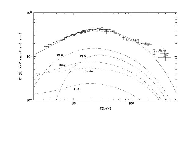
Figure 6: The XRB spectrum above 3 keV: comparison between model (continuous line) and data. The data above 3 keV are taken from a compilation of the best experimental results $\!{}^{{\bf?}}$. The curves, labelled with values of log $N_{H}$, show the expected contribution from AGNs with different amount of intrinsic absorption.

As an example, we show in Figure 6 the results of a fit to the XRB spectrum obtained by Comastri et al. $\!{}^{{\bf?}}$. The main ingredients of this model, which takes into account the observed spectral properties of different classes of AGNs over a broad energy range, are the following:

a) The X–ray primary continuum spectrum of AGNs is described by two power laws with spectral indices $\alpha$ = 1.3 below 1.5 keV and $\alpha$ = 0.9 above this energy. A Compton reflection component (50% of the primary spectrum) has been added in the continuum of the low luminosity AGNs $\!{}^{{\bf?}}$ (i.e. Seyfert 1 galaxies), while no such component has been considered in high luminosity AGNs $\!{}^{{\bf?}}$. In agreement with the OSSE data $\!{}^{{\bf?}}$, the power law spectrum is assumed to be exponentially cut–off at an e–folding energy of about 320 keV.

b) As required by the adopted unified scheme, the intrinsic X–ray spectrum of type 2 AGNs is assumed to be the same as the spectrum of type 1 AGNs, but modified by absorption effects $\!{}^{{\bf?}}$. A distribution of $N_{H}$, i.e. the column density of the absorbing material, in the range $10^{21}-10^{25}$ atoms $cm^{-2}$, consistent with the observed distribution $\!{}^{{\bf?}}$ is derived.

With these assumptions, the fit shown in Figure 6 has been obtained by integrating the local X–ray luminosity function of AGNs and assuming a luminosity evolution up to z $\sim$ 2. At higher redshift the X–ray luminosity function has been assumed to remain constant. This model, as well as other models based on similar assumptions (see, for example, $\!{}^{{\bf?}}$), fits the XRB spectrum well up to $\sim$ 100 keV, while it underpredicts the data at $\sim$ 500 keV by a factor of a few. It has been shown in $\!{}^{{\bf?}}$ that at this energy the contribution from a different AGN population, namely flat spectrum radio quasars and “MeV blazars”, is already substantial. These objects are likely to contribute most of the observed background in the energy range $1-10^{3}$ MeV.

As shown in the figure, the model predicts that in the hard X–ray band most of the contribution to the XRB comes from significantly absorbed objects, which are almost absent in the soft band, even at the faintest ROSAT limit. As a consequence, a significant test for this model would be the comparison of its predictions with the results of optical identifications of a complete sample of X–ray sources selected at low fluxes in the hard X–ray band.

\begin{picture}(6.0,6.0)\centerline{\hbox{\psfig{width=213.39566pt}}} \end{picture}

Figure 7: The 2–10 keV log(N)–log(S). The circles represent the counts derived from the 60 ASCA sources discussed in $\!{}^{{\bf?}}$; the square shows the preliminary results of a different ASCA survey in a more limited sky area $\!{}^{{\bf?}}$; the triangle shows the extragalactic surface density from the HEAO-1 survey $\!{}^{{\bf?}}$. The curves show the predictions for various classes of objects from the model discussed in  $\!{}^{{\bf?}}$.

Recently, ASCA data have been used $\!{}^{{\bf?}}$ to derive the 2–10 keV log(N)–log(S) down to fluxes slightly below $10^{-13}erg~{}cm^{-2}~{}s^{-1}$. This data, based on 60 X–ray sources detected in ASCA images, is shown in Figure 7 together with the predictions for various classes of objects from the Comastri et al. model. As discussed in Cagnoni et al. $\!{}^{{\bf?}}$, if one uses the ROSAT log(N)–log(S) and the average spectral properties of the ROSAT sources to predict the ASCA log(N)–log(S), the prediction falls a factor $\sim$ 2 below the data at a flux of the order of $\sim$ $10^{-13}erg~{}cm^{-2}~{}s^{-1}$. On the other hand, as shown in the figure, the data are in good agreement with the predictions of the Comastri et al. model. The dashed line in Figure 7 shows that a significant fraction of the AGNs in this ASCA survey, and an even larger fraction at fainter fluxes, should be substantially absorbed and therefore their optical counterparts are expected to have optical spectra typical of Seyfert 2 galaxies. A program to optically identify these sources has already started, but the large positional uncertainty ($\sim$ 2 arcmin) together with the relatively faint expected magnitudes of the optical counterparts will make it difficult to obtain unambiguous identifications. Fortunately, the situation will soon improve with the missions to be launched in the next few years, as for example AXAF and XMM. These missions will provide much fainter samples of hard X–ray selected sources, with significantly better positional uncertainty (of the order of 1–2 arcsec for AXAF and 5–10 arcsec for XMM). These faint hard samples will be complemented by the bright all-sky sample from the ABRIXAS survey. The optical identifications of these sources with the 8m class telescopes will be able to conclusively test the predictions of our current models and, hopefully, finally settle the question of the X-ray background.

5 Conclusions

In the last decade there has been a substantial improvement in our understanding of both the X-ray background and the spectra of active galactic nuclei. To first order we can regard the problem of the X-ray background as solved. For the first time since its discovery we can explain the bulk of the X-ray background over a wide range of energies (0.1-100 keV) as due to a known class of sources, namely unabsorbed and absorbed active galactic nuclei, whose statistical properties like average spectra, absorption distribution, luminosity function etc. are consistent with those measured locally and which are strongly evolving with cosmic time.

In the soft X-ray band, mainly based on ROSAT deep surveys, the majority of identified sources down to the faintest fluxes are indeed AGNs and the background models can account for all observable constraints like log(N)-log(S) function, redshift distribution, average spectral index etc. Observations at harder X-ray energies, e.g. by ASCA, are consistent with this picture. However, only deeper survey observations with the next generation of sensitive X-ray observatories with good angular resolution in the harder X-ray band (i.e. AXAF and XMM) and optical follow-up spectroscopy from 8-10m telescopes will be able to unambiguously confirm the AGN XRB model and to tighten the constraints on some of the still relatively uncertain model parameters.

References

References

- [1] Giacconi R. and Burg R. 1992, in The X–Ray Background, X. Barcons and A.C. Fabian eds., (Cambridge: Cambridge Univ. Press), 3.
- [2] Giacconi R., Gursky H., Paolini F.R. and Rossi B.B. 1962, Phys.Rev.Letters, 9, 439.
- [3] Schwartz D.A. 1980, Phys.Scripta, 21, 644.
- [4] Tanaka Y. 1992, in X–Ray Emission from Active Galactic Nuclei and the Cosmic X–Ray Background, W. Brinkmann and J. Trümper eds., MPE Report 235, 303.
- [5] Marshall F.E. et al. 1980, Ap.J., 235, 4.
- [6] Mushotzky R.F. 1984, Advances in Space Research, Vol. 3, no. 10–12, p.157.
- [7] Setti G. and Woltjer, L. 1973, in IAU Symposium No. 55, X- and Gamma–Ray Astronomy, H. Bradt and R. Giacconi eds., (Reidel, Dordrecht), p. 187
- [8] Tananbaum R. et al. 1979, Ap.J.Letters, 234, L9.
- [9] Zamorani G. et al. 1981, Ap.J., 245, 357.
- [10] Giacconi R. et al. 1979, Ap.J.Letters, 234, L1.
- [11] Griffiths R.E. et al. 1983, Ap.J., 269, 375.
- [12] Primini F.A. et al. 1991, Ap.J., 374, 440.
- [13] Hamilton T.T., Helfand D.J. and Wu X. 1991, Ap.J., 379, 576.
- [14] Setti G. 1985, in Non–Thermal and Very High Temperature Phenomena in X–Ray Astronomy, G.C. Perola and M. Salvati eds., p. 159.
- [15] Giacconi R. and Zamorani G. 1987, Ap.J., 313, 20.
- [16] Mather J.C. et al. 1990, Ap.J.Letters, 354, L37.
- [17] Mather J.C. et al. 1994, Ap.J., 420, 439.
- [18] Wright et al. 1994, Ap.J., 420, 450.
- [19] Pfeffermann E. et al. 1986, SPIE, 733, 519.
- [20] Soltan A.M. 1991, MNRAS, 250, 241.
- [21] Hamilton T.T. 1992, in The X–Ray Background, X. Barcons and A.C. Fabian eds., (Cambridge: Cambridge Univ. Press), 138.
- [22] Briel U.G. et al. 1988, SPIE, 982, 401.
- [23] Hartner G. 1986, Diplomarbeit TU München
- [24] Hasinger G. et al. 1993, A&A 275, 1.
- [25] Lockman F.J., Jahoda K. and McCammon D. 1986, Ap.J., 302, 432.
- [26] Marano B., Zamorani G. and Zitelli V. 1988, MNRAS, 212, 111.
- [27] Schmidt M. and Green R.P. 1983, Ap.J., 269, 352.
- [28] de Ruiter H. et al. 1997, A&A, 319, 7.
- [29] Hasinger G. et al. 1994, Legacy, 4, 40; MPE/OGIP Calibration Memo.
- [30] David F.R. et al. 1996, in The ROSAT Users Handbook
- [31] Williams R.E. et al. 1996. A.J., 112, 1335.
- [32] Hasinger et al. 1997, A&A, submitted.
- [33] Hasinger G., Schmidt M. and Trümper J. 1991, A&A, 246, L2.
- [34] Branduardi-Raymont G. et al. 1994, MNRAS, 270, 947.
- [35] Vikhlinin A. et al. 1995, Ap.J., 451, 553.
- [36] Barcons X. et al. 1994, MNRAS, 268, 833.
- [37] Mason, K. et al. 1996, priv. comm.
- [38] Shanks T. et al. 1991, Nature, 353, 315.
- [39] Georgantopoulos I. et al. 1996, MNRAS, 280, 276.
- [40] Gioia I.M. et al. 1990, Ap.J.Suppl., 72, 567.
- [41] Boyle B.J. et al. 1994, MNRAS, 260, 49.
- [42] Page M.J. et al. 1996, MNRAS, 281, 579.
- [43] Jones L.R. et al. 1996, MNRAS, submitted, (astro-ph/9610124).
- [44] Boyle B.J. et al. 1995, MNRAS, 272, 462.
- [45] Griffiths R.E. et al. 1996, MNRAS, 281, 71.
- [46] Roche N. et al. 1995, MNRAS, 273, L15.
- [47] McHardy I.M. et al. 1997, MNRAS, submitted, (astro-ph/9703163)
- [48] Hasinger G. 1996, A&A Suppl., 120, C607.
- [49] Schmidt M. et al. 1997, A&A, submitted.
- [50] Fabian A.C. and Barcons X. 1992, ARA&A, 30, 429.
- [51] Soltan A. and Hasinger G. 1994, A&A, 288, 77.
- [52] Burg R. et al. 1992, A&A, 259, L9.
- [53] Ashby M.N.L. et al. 1996, Ap.J., 456, 428.
- [54] Mushotzky R.F. 1997, in Mass Ejection from AGN, in press, (astro-ph/9705004).
- [55] Pounds K.A. et al. 1990, Nature, 344, 132.
- [56] Nandra K. 1991, Ph.D. Thesis, Leicester University.
- [57] Schwartz D.A. and Tucker W.H. 1988, Ap.J., 332, 157.
- [58] Morisawa K., Matsuoka M., Takahara F. and Piro L. 1990, A&A, 263, 299.
- [59] Fabian A.C., George I.M., Miyoshi S. and Rees M.J. 1990, MNRAS, 242, 14P.
- [60] Terasawa N. 1991, Ap.J.Letters, 378, L11.
- [61] Rogers R.D. and Field G.B. 1991, Ap.J.Letters, 370, L57.
- [62] Zdziarski A.A., Zycki P.T., Svensson R. and Boldt E. 1993, Ap.J., 405, 125.
- [63] Madau P., Ghisellini G. and Fabian A.C. 1994, MNRAS, 270, 117.
- [64] Comastri A., Setti G., Zamorani G. and Hasinger G. 1995, A&A, 296, 1.
- [65] Antonucci R.J. 1995, ARA&A, 31, 473.
- [66] Setti G. and Woltjer L. 1989, A&A, 224, L21.
- [67] Gruber D.E. 1992, in The X–Ray Background, X. Barcons and A.C. Fabian eds., (Cambridge: Cambridge Univ. Press), 44.
- [68] Williams O.R. et al. 1992, Ap.J., 389, 157.
- [69] Zdziarski A.A. et al. 1995, Ap.J.Letters, 438, L63.
- [70] Awaki H., Koyama K., Inoue H. and Halpern J.P. 1991, PASJ, 43, 195.
- [71] Schartel N. et al. 1997, A&A 320, 696.
- [72] Celotti A., Fabian A.C., Ghisellini G. and Madau P. 1996, MNRAS, 277, 1169.
- [73] Comastri A., Di Girolamo T. and Setti G. 1996, A&A Suppl., 120, C627.
- [74] Cagnoni I., Della Ceca R. and Maccacaro T. 1997, Ap.J., submitted.
- [75] Ogasaka Y. 1997, in X–ray Imaging and Spectroscopy of Cosmic Hot Plasmas, F. Makino and K. Mitsuda eds., 25.
- [76] Piccinotti G. et al. 1982, Ap.J., 253, 485.