The Energy Spectra and Relative Abundances of Electrons
and Positrons in the Galactic Cosmic Radiation

Abstract

Observations of cosmic-ray electrons and positrons have been made with a new balloon-borne detector, HEAT (the “High-Energy Antimatter Telescope”), first flown in 1994 May from Fort Sumner, NM. We describe the instrumental approach and the data analysis procedures, and we present results from this flight. The measurement has provided a new determination of the individual energy spectra of electrons and positrons from 5 GeV to about 50 GeV, and of the combined “all-electron” intensity ${\rm(e^{+}+e^{-})}$ up to $\sim 100$ GeV. The single power-law spectral indices for electrons and positrons are $\alpha=3.09\pm 0.08$ and $3.3\pm 0.2$, respectively. We find that a contribution from primary sources to the positron intensity in this energy region, if it exists, must be quite small.

PSU-PAL-97-1

1 Introduction

Electrons and positrons are a relatively rare component of the cosmic radiation, but are distinct from all other cosmic-ray particles because of their low mass and the absence of hadronic interactions with the constituents of the interstellar medium. Previous measurements of electrons ${\rm(e^{+}+e^{-})}$ up to roughly 1000 GeV ([Prince 1979, Nishimura et al. 1980, Golden et al. 1984, Tang 1984]) have shown that their intensity amounts to about 1% of the flux of protons around 10 GeV, but decreases more rapidly with energy ($\propto E^{-3.1}$) than the proton spectrum ($\propto E^{-2.7}$). Separate measurements of positrons and electrons have only been possible at much lower energies and have indicated a “positron fraction” (${\rm e^{+}/(e^{+}+e^{-})}$) of a few percent in the region 1-10 GeV ([Fanselow et al. 1969, Buffington et al. 1975, Golden et al. 1996, Barbiellini et al. 1996]). Some measurements have indicated an increase above about 10 GeV ([Agrinier et al. 1969, Müller & Tang 1987, Golden et al. 1987, Golden et al. 1994]). These observations have led to a number of conclusions, but have also left some key questions unanswered:

1) The predominance of negative electrons can only be explained if electrons are accelerated by primary sources. The alternate production mechanism, as secondary particles from interstellar nuclear interactions of hadronic cosmic rays (mostly through the $\pi^{\pm}\rightarrow\mu^{\pm}\rightarrow{\rm e}^{\pm}$ decay), would yield negative and positive electrons in about equal proportions, and thus can only account for a small portion of the total ${\rm e^{\pm}}$ flux. It is worth pointing out that electrons are the only cosmic-ray component for which an extragalactic contribution can be excluded with certainty: energy losses through Compton interactions with the 2.7K background radiation preclude their propagation through intergalactic distances.

2) The steepness of the observed energy spectrum of electrons is usually explained as a consequence of radiative energy losses during propagation through the interstellar medium: inverse Compton scattering with photons and synchrotron radiation in the interstellar magnetic fields. Assuming that electrons are accelerated with the same energy spectrum at the source as nuclei ($\propto E^{-2.15}$, [Müller et al. 1991, Swordy et al. 1993]) the observed spectral slope is roughly consistent with the galactic containment time of $\sim 10^{7}$ years of nuclei at GeV energies. However, there are several problems with this interpretation: First, the energy spectrum of electrons at the source is not known a priori, nor is it known that electrons and nuclei originate at the same acceleration sites. Second, it has been pointed out ([Tang 1984]) that the energy dependence ($\propto E^{-0.6}$) of the containment time observed for nuclei may be difficult to reconcile with the observed shape of the electron spectrum. Third, the “leaky box” assumption inherent in these explanations should not be applied to electrons, as it requires an unreasonably high density of electron sources in the galactic disk ([Cowsik & Lee 1979]).

3) The small flux of positrons appears to be essentially consistent with a secondary origin. If this is true, the production spectrum of positrons can be calculated from the known flux of primary nuclei ([Protheroe 1982]). Positrons would be produced continuously throughout the galactic disk, and the leaky box model could more easily be taken as an approximation for their propagation through the galaxy. In any case, a direct comparison between the production spectrum and the observed positron spectrum would permit a quantitative study of the propagation mechanism. However, it must first be ascertained that indeed all positrons are of secondary origin. The previously observed increase in the positron fraction has led to much speculation about the appearance of primary positrons at high energy (e.g. [Harding & Ramaty 1987, Aharonian & Atoyan 1991, Dogiel & Sharov 1990, Tylka 1989, Turner & Wilczek 1990, Kamionkowski & Turner 1991]). Recent results ([Barwick et al. 1995, Barwick et al. 1997a]) have not confirmed this increase, but have not yet shown conclusively that the positron flux is entirely free of primary contributions.

It is clear from these considerations that many of the open questions can only be answered through measurements of electrons and positrons separately, and over as large an energy range as possible. This was the motivation for the construction of the High-Energy Antimatter Telescope (HEAT), an instrument that utilizes a large superconducting magnet spectrometer to separate positive and negative particles, and that incorporates powerful techniques to identify electrons and positrons and to reject hadronic background. A first balloon flight of HEAT was conducted in 1994. In the following, we shall describe this measurement and the data analysis technique, and we shall present and discuss the results.

2 Flight

The first balloon flight of the HEAT e^± instrument took place on 1994 May 3-5, from Fort Sumner, New Mexico, and data were collected at float altitude for about 29 hours. The payload reached a maximum altitude of 36.5 km and drooped to a minimum of 33 km at night, as illustrated in Figure 1. Over the course of the flight, the payload drifted between vertical geomagnetic cutoff rigidities of 4 GV and 4.5 GV, latitudes of $33.35^{\circ}$ N and $35.3^{\circ}$ N and longitudes of $100.0^{\circ}$ W and $104.3^{\circ}$ W. The instrument was recovered undamaged near Wellington, Texas.

fig1

3 Instrument Description and Performance

The expected intensity of cosmic-ray positrons is quite low, of the order of $10^{-4}$ of the total cosmic-ray intensity at comparable energies. A successful measurement then necessitates a detector with large sensitive area to yield statistically significant data, and with very high discrimination power against the overwhelming proton background. This is accomplished in the HEAT instrument, shown in Figure 2, through the combination of a superconducting magnet spectrometer (using a drift-tube hodoscope (DTH) tracking chamber) with particle identifiers employing a time-of-flight system (TOF), a transition-radiation detector (TRD), and an electromagnetic calorimeter (EC). A thorough description of the instrument appears elsewhere ([Barwick et al. 1997b]), and the following just gives a brief summary of the apparatus and its performance.

fig2

3.1 Time-of-Flight System

The TOF measures the velocity of the particle, distinguishes downward from upward-going (albedo) particles, and measures the magnitude of the particle’s charge. The rejection of upward-going particles is necessary as these would otherwise appear as particles of the opposite charge in the magnet spectrometer. Through the measurement of the magnitude of the charge, singly-charged particles are identified and discriminated from helium and heavier nuclei.

The TOF consists of four scintillator slabs on top of the instrument, each with an active area of 100 cm $\times$ 25 cm, and of the top three scintillation counters of the EC (described below). Throughout the instrument, photomultiplier tubes (PMT) are used that are resistant to the magnetic fringe fields.

The PMT signals are both charge- (ADC) and time- (TDC) digitized, and the particle’s charge is determined from the ADC values measured with the top scintillator slabs, each of which has a PMT on either end. Figure 3 shows the charge distribution obtained for flight data, with the criteria for selecting singly-charged particles shown as dashed lines (and summarized in Table 1). The charge resolution obtained is 0.11 charge units, which is sufficient to provide good rejection of He events. The TDC values, after corrections for the path length through the instrument, give the particle’s velocity, with a resolution of 0.13 c (where c is the speed of light). Figure 3 shows the velocity distribution obtained for flight data, and indicates the selection criteria used for the analysis.

fig3

3.2 Transition-Radiation Detector

The transition-radiation detector is used to distinguish electrons and positrons from hadrons. It is comprised of 6 modules, each consisting of a polyethylene-fiber radiator and a multiwire proportional chamber (MWPC). The MWPCs contain a gas mixture of xenon:methane (70:30) and produce signals on both the anode wires and on cathode strips. The total charge deposited in the chamber is read from the cathode strips and pulse-height analyzed (“PHA” analysis), while the current signal is read from the anode wires in 25 nsec-wide time slices, which are digitized into three different threshold levels (“time-slice” analysis).

Charged particles of high Lorentz factor ($\gamma>10^{3}$) produce transition-radiation (TR) x-rays (5–30 keV) in the radiator, which are subsequently detected by the MWPC. This x-ray signal is superimposed on the signal due to ionization energy loss of the parent particle. In the energy range of 5–50 GeV, electrons produce a saturated TR signal, while protons and pions produce none, thereby permitting a discrimination between these species.

3.2.1 PHA Analysis

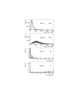
Figure 4: PHA and Time-Slice probability distributions for protons and electrons

A maximum-likelihood technique is used to analyze the PHA signals ([Cherry et al. 1974]). To this end, first the probability distributions for the pulse heights in the MWPC’s must be determined, using clean populations of electrons and protons. The electron sample is obtained by selecting events with negative rigidity in the magnet spectrometer (described below), and a shower profile in the EC consistent with an electromagnetic shower (also described below). The proton sample is obtained by selecting events with positive rigidity and which have shower profiles inconsistent with an electromagnetic shower. The validity of this procedure has been verified with accelerator calibrations at Fermilab. Gain differences between the TRD chambers are corrected for, as are temporal variations (30%) in the chamber gains caused by temperature and pressure changes inside the instrument gondola, spatial non-uniformities (20%), and the relativistic rise of the proton ionization signal. The upper two panels of Figure 4 show the PHA probability distributions P_e for electrons and P_p for protons.

fig4

For the subsequent data analysis, each event, characterized by the MWPC pulse heights $x_{i}$ ($i=$1,…,6), is compared with the probability distributions, and a likelihood ratio $L_{\mbox{\scriptsize\it PHA}}$ is formed:

$$L_{\mbox{\scriptsize\it PHA}}=\prod_{i=1}^{6}\frac{P_{e}(x_{i})}{P_{p}(x_{i})}.$$

Figure 5 shows as a dashed line labeled “PHA” the electron and proton efficiencies obtained by applying a selection on the PHA likelihood ratio.

fig5

3.2.2 Time-Slice Analysis

The time-slice technique makes use of the fact that an x-ray photon absorbed in the MWPC generates a highly localized “ionization cluster” in the chamber, which then drifts to the anode wires and produces a “spike” in the time structure of the anode signal. In the analysis, again, a likelihood ratio $L^{\prime}_{\mbox{\scriptsize\it TS}}$ is constructed, using the appropriate single-chamber probability distributions $P^{\prime}_{e}$ and $P^{\prime}_{p}$. These distributions are based on the number of time slices above each threshold level, and the positions, heights, and number of clusters in the time-slice distribution, after the gain corrections described above are applied. The lower two panels of Figure 4 show the time-slice probability distributions obtained for electrons and protons. Figure 5 shows as a dotted line labeled “Time-Slice” the electron and proton efficiencies obtained by applying a selection on the time-slice likelihood ratio.

The likelihood ratios $L_{\mbox{\scriptsize\it PHA}}$ and $L^{\prime}_{\mbox{\scriptsize\it TS}}$, are combined to form a total ratio: $L_{\mbox{\scriptsize\it Total}}=L_{\mbox{\scriptsize\it PHA}}\cdot L^{\prime}_{\mbox{\scriptsize\it TS}}$. Figure 6 shows the distribution of $L_{\mbox{\scriptsize\it Total}}$ together with the selection criterion used to identify electrons ($L_{\mbox{\scriptsize\it Total}}>10^{3}$, or dashed line in the figure). With this criterion, electrons are retained with an efficiency $\epsilon_{e}=88\%$ and protons with an efficiency $\epsilon_{p}=0.59\%$, corresponding to a proton rejection power of 170. This is illustrated in Figure 5 as a solid line labeled “Total.”

fig6

3.3 Magnet Spectrometer

The magnet spectrometer is used to measure the rigidity $R={pc\over Ze}$ and charge sign of a traversing charged particle, and consists of a two-coil warm-bore superconducting magnet and a precision tracking detector utilizing drift tubes. The magnet produces an approximately uniform field of central value 1 T. The fiducial volume within the magnet bore measures 50 cm $\times$ 50 cm $\times$ 61 cm. The tracking system consists of 479 drift tubes of 2.5 cm diameter, arranged in 26 rows; 18 rows (of which 17 were operational during the flight) contain tubes parallel to the magnet axis, defining the bending view, and 8 contain tubes perpendicular to the magnet axis, defining the non-bending view. The drift gas mixture used is CO₂:hexane (96:4).

The DTH determines the particle trajectory by measuring the drift times of the ionization tracks in each tube hit, from which, using a “time-to-space” function, the impact parameters (distance of closest approach to wire) are found. The trajectory of the particle in three dimensions is reconstructed from the impact parameters using a modified version of the CERN program libraries’ MOMENTM algorithm ([Wind 1974]). Figures 7 and 8 show the residuals from the tracks reconstructed for flight data, as a distribution and as a function of radius, respectively. A signal is not used in the track fit if it lies more than one tube diameter away from the reconstructed trajectory, or if it has a residual that is worse than 6 times the average residual for the track. Also removed are signals corresponding to an impact parameter smaller than 2 mm, a region where the tracking capabilities of the drift tubes are poor due to the nature of the electron-ion pair statistics and the increased drift speed near the wire. The single-tube resolution achieved is about 70 $\mu$m.

fig7

fig8

The performance of the magnet spectrometer is characterized by the maximum detectable rigidity (MDR). The MDR is defined as that rigidity where the RMS error in the sagitta measurement is equal to the sagitta of the track, and is computed on an event-by-event basis. The MDR distribution for electron events, given in Figure 9, shows that a mean MDR of 170 GV is achieved. The MDR yields the relative RMS error in the rigidity: $\sigma_{R}/R=R/MDR$. Thus, an MDR of 170 GV provides for a rigidity determination with an at least $3\sigma$ accuracy up to $\sim$ 60 GV. In the analysis of the flight data, the selections $R/MDR<0.25$ and $MDR>60$ are imposed to ensure meaningful results.

fig9

3.4 Electromagnetic Calorimeter

The electromagnetic calorimeter measures the energy of electrons and discriminates against hadrons. The EC consists of ten lead plates, each 0.9 radiation length thick and 50 cm $\times$ 50 cm in area, and each followed by a plastic scintillator.

Electrons deposit most of their energy in the EC, with well-understood shower profiles that provide a measure of their energy. Protons and other hadrons, on the other hand, rarely interact in the EC, as it represents only about 0.3 proton interaction lengths, and if a nuclear interaction occurs, the longitudinal shower profile is usually quite different from that of an electron. Therefore, the EC also provides powerful discrimination against protons.

In order to reconstruct the electron primary energy from the shower profile, Monte Carlo simulations have been carried out using the CERN program libraries’ GEANT package ([Brun et al. 1994]). The results of these simulations have been verified through accelerator calibrations ([Torbet et al. 1993]). A covariance analysis is applied to the Monte Carlo events, providing the cross-correlations between the signals obtained in each of the layer pairs as a function of energy. Figure 10 shows, for 10 GeV simulated electrons, the distribution of energies reconstructed by this covariance analysis. The correlation matrices generated by the covariance analysis of Monte Carlo events are then applied to flight data to determine the particle energies. The fractional energy resolution achieved is about 10% for the energy range of interest.

fig10

During the balloon flight, an event trigger is employed (see below) that requires a minimum energy deposition in the EC, and thereby removes most non-interacting protons. In order to discriminate against the remaining proton events with the EC, a $\chi^{2}$ measure of the agreement between the observed and expected shower profile, generated by the covariance analysis, is determined for each event. In addition, the shower start depth $t$ is derived from a separate profile analysis of the shower, and events with $t>0.89$ radiation length are rejected. Finally, agreement between the energy $E$ measured by the EC, and the momentum $p$ measured by the magnet spectrometer is demanded. Figure 11 shows the electron and proton efficiencies obtained for flight data by imposing all of these requirements. The selection criteria chosen for the analysis are summarized in Table 1, and yield for the combination of shower counter and magnet spectrometer a proton rejection power of 460 at an electron efficiency of 97%. Combined with that of the TRD (see above), the total rejection power of the instrument against protons is nearly $10^{5}$.

fig11

3.5 Instrument Trigger

The instrument trigger requires a through-going particle which deposits a signal larger than that of a 0.5 GeV electron in the EC. This excludes non-interacting protons. In addition, a minimum number of hits in the DTH is required. A “fast” trigger is formed by the coincidence of signals in the top and bottom TOF scintillators, and of a signal above threshold in the sum of the lower seven EC layers. A “slow” confirming trigger is required within 1.5 $\mu$sec thereafter, based on the occurrence of a three-fold majority of hits in the first, fifth, and last two rows of tubes in the bending plane. In order to obtain a sample of non-interacting protons, the EC sum threshold requirement is removed for a small percentage (2%) of the events.

4 Electron Selection

4.1 Event Filtering

The initial data analysis stage involves examining the DTH hits for clean single-particle events. A rough estimate of the trajectory is made by performing a quadratic fit to the impact parameters in both the bending and non-bending views. Signals from tubes well outside this fit are discarded. Events in which tracks cannot be identified in the DTH through this procedure are rejected. Most events eliminated at this stage result from interactions of particles that penetrate the instrument from the sides.

Tracks which pass the initial DTH filter are then analyzed using the modified MOMENTM algorithm, which determines the particle’s rigidity from the measured track points. A $\chi^{2}$ parameter, generated by comparing the measured track points with the fit, is used to reject events with large tracking errors. In addition, events are rejected based on the average residuals associated with the track, as well as on the number of tubes retained in the final fit in the bending and non-bending views. Finally, the MDR requirements described in Section 3.3 are imposed. Table 1 summarizes all of the track cleanliness requirements.

all_cuts

4.2 Template Fits

Electron selection criteria are applied to events that satisfy the track cleanliness requirements. As discussed, these include selections on the magnitude of the particle charge, the TRD total likelihood ratio, the EC covariance analysis $\chi^{2}$ parameter, the shower start depth, and reconstructed energy. In order to maximize the statistics of the results, the electron selection criteria have been chosen relatively loosely, requiring that the number of background protons be less than 25% of the number of accepted positrons. Table 1 summarizes the selections used.

For events meeting the electron selection criteria, distributions of the ratio of the measured energy $E$ determined by the EC, and the momentum $p$ determined by the magnet spectrometer, are generated. Figure 12 shows these $E/p$ distributions for electrons and positrons in five top-of-the-atmosphere (ToA) energy intervals. (The top-of-the-atmosphere energy $E_{ToA}$ is obtained from the measured energy $E$ by correcting for atmospheric bremsstrahlung losses according to the procedure described in Section 5.2.) The differences in $E/p$ between positrons and residual background protons is evident, with the positron distribution peaking at +1, and that for protons peaking at about +0.5. The tails at high $\left|E/p\right|$ values in the electron or positron distributions are due to bremsstrahlung losses in the material above the DTH, which result in a reduced rigidity in the spectrometer while the entire energy (of the e^± plus bremsstrahlung photons) is usually recorded in the EC.

fig12

A fit to the $E/p$ distributions for electrons and positrons is performed to obtain the number of electrons and positrons, and to estimate and subtract the residual proton background. The $E/p$ distribution for negative electrons, which can be taken as background free, is used to obtain a template of the expected $E/p$ distribution for e^±. The $E/p$ distribution for background protons is obtained by inverting the TRD selection to select interacting protons (see Table 1). Both template distributions are smoothed, and used to fit the $E/p$ distribution for positrons, shown as the solid curves in Figure 12. A Bayesian treatment is then used to estimate the electron, positron and proton counts, with prior probability distributions assumed to be flat for the electron, positron and proton background counts, and with conditional distributions taken from the template fits. The electron and positron counts resulting from this procedure are listed in Table 1. The uncertainties given in the table are 16 and 84% Bayesian limits. For the energy range 50–100 GeV, the ability of the magnetic spectrometer to determine the direction of bending is reduced as the uncertainty on the sagitta of the track is comparable to the sagitta itself. Therefore, in this energy range, electron events are selected without the rigidity-related selection criteria of Table 1, and electrons are not distinguished from positrons.

elec_numb

As a test to verify the degree of potential residual contamination of the positron counts by interacting hadrons, the electron selection criteria were varied from very loose to very restrictive. In all but the loosest sets of selection criteria, the electron and positron counts were reduced or augmented in the same proportion, indicative of little, if any, residual contamination.

5 Absolute Energy Spectra

The absolute differential energy spectra of cosmic-ray primary electrons or positrons are obtained from the raw electron or positron counts $\Delta N$ of Table 1 by calculating:

$$j_{pri}(\bar{E})\approx\frac{f_{ToA}\Delta N}{\Delta E\>\mbox{\large$\epsilon$}\,\Omega\,A\,\Delta t}-j_{sec}(\bar{E})$$ (1)

with

$$\bar{E}=\frac{\int_{E_{i}}^{E_{j}}E\,E^{-\alpha}\,dE}{\int_{E_{i}}^{E_{j}}E^{-\alpha}\,dE}$$

$$\Delta E=\int_{E_{i}}^{E_{j}}E^{-\alpha}\,dE/\bar{E}^{-\alpha},$$

where an atmospheric secondary (sec) component is subtracted to obtain the primary (pri) component. In equation (1), $\epsilon\Omega A$ is the instrumental acceptance, $\Delta t$ is the live time, $E_{i}$ and $E_{j}$ are the lower and upper bounds of each ToA energy interval, respectively, $\bar{E}$ is the weighted average ToA energy in this interval, $\Delta E$ is the weighted ToA energy interval, $f_{ToA}$ is a correction factor related to the transformation of the energy scale to the top of the atmosphere, which will be described in Section 5.2, and $\alpha$ ($\approx 3.1$ for primary particles and $\approx 3.2$ for atmospheric secondaries) is the power-law spectral index.

The live time $\Delta t$ of the detector is measured in flight with a scaler which counts clock cycles only while the instrument is available for triggers and not busy processing an event following a trigger. Periods of instability of the instrument’s performance are discarded, and a total live time of $(18.04\pm 0.04)$ hours at float altitude is obtained. This live time includes losses due to transmission errors and data-unpacking errors from glitches in the electronics of individual subsystems.

5.1 Monte Carlo Simulations

Some of the quantities in equation (1) are determined with a full Monte Carlo (MC) simulation of the HEAT instrument, based on the GEANT software package, and including the actual detector configuration and the experimentally-determined fluctuations in detector response. For instance, the MC simulation is used to calculate the instrumental acceptance for electrons, i.e., the product of the absolute efficiency $\epsilon$ and the geometrical aperture $\Omega A$. The MC-calculated efficiencies are compared to experimental quantities where possible, and in some cases renormalized to ensure agreement. For example, the TRD electron selection efficiency is determined by obtaining a set of electron events based on EC, TOF and DTH information, and measuring the fraction of such events that satisfy the TRD likelihood ratio requirement. In addition, a visual inspection of several hundred raw experimental and simulated electron events revealed that about 65% of experimental events are accepted by the analysis, whereas 81% of simulated events are accepted. The instrumental acceptance determined by the MC is therefore corrected by a “scanning” efficiency factor of $\epsilon_{\mbox{\scriptsize\it scan}}$ $=0.65/0.81=0.80\pm 0.08$, the uncertainties being an estimate of the spread of values due to independent scannings.

Table 1 lists, for each energy interval, the acceptances calculated with the MC, including the $\epsilon_{\mbox{\scriptsize\it scan}}$ correction. The geometrical aperture, uncorrected for efficiencies, is about 495 $\mbox{cm}^{2}\,\mbox{sr}$. This indicates an average electron acceptance efficiency of about 37%. In Table 1, the acceptance uncertainties are obtained by adding in quadrature the uncertainties in the individual efficiency factors. The increased acceptance of the highest energy bin derives from an increased efficiency due to a different set of selection criteria used in this energy range, as indicated in Table 1.

acc_liv

A comparison of experimental and simulated $E/p$ distributions revealed a systematic energy calibration offset in the flight data. Specifically, the experimentally-determined

$\left|E/p\right|$ peak for electrons is shifted upwards by about 14%, whereas the Monte Carlo simulation predicts a shift of only 4% due to the bremsstrahlung energy losses. The 10% discrepancy appears to be due to a systematic bias in the conversion of the ADC values of the EC into numbers of minimum-ionizing particles. This energy-scale shift is corrected for in Figure 12.

The measured energy spectrum is shifted without a change in spectral index due to the finite, but roughly constant, energy resolution of the EC. The Monte Carlo simulation shows that of these events which have a true initial energy in a given energy bin, a fraction of 2 to 6% are reconstructed by the analysis into the next higher-energy bin, while 22 to 32% are reconstructed into the adjacent lower-energy bin. This “spillover” effect reduces the reconstructed energy spectrum by about 10% in overall intensity as compared to the true primary spectrum. The final results have been corrected for this effect. Only events with ToA energies above 5 GeV, well above the geomagnetic rigidity cutoff at $\sim 4.5$ GV, are retained in the analysis.

5.2 Atmospheric Corrections

The electron spectrum measured at balloon altitudes is comprised of primary cosmic-ray electrons and atmospheric secondary electrons. The secondary component arises as a result of interactions of hadrons or primary electrons within the atmosphere, as well as reentrant albedo electrons. Reentrant albedo particles are significant only below the geomagnetic cutoff energy. To determine the secondary flux generated in the atmosphere, a Monte Carlo simulation utilizing the CERN libraries’ FLUKA hadronic interaction algorithm ([Fassó et al. 1993]) is used. For this calculation, a primary proton spectrum with a power-law index of 2.74 is assumed ([Seo et al. 1991]). Secondaries produced by primary electrons do not contribute significantly. To account for the contribution of heavy primary nuclei, the simulated intensity of atmospheric secondaries is multiplied by 1.2 ([Orth & Buffington 1976]). The total intensity of 10 GeV secondary electrons and positrons at 6 g/cm² is found to be 0.006 (GeV s sr m²)^-1. This corresponds to overall corrections to the positron intensity of 20–30%, and to the electron intensity of 1–2%, at the energies of interest. The absolute atmospheric intensities at an average atmospheric depth of 5.7 g/cm² for electrons and positrons are also presented in Table 1, for each energy interval.

atm_sec

As a test of the reliability of the MC calculation, atmospheric growth curves for electrons and positrons are measured during the flight. The positron fraction as a function of depth in the atmosphere is shown in Figure 13, for two separate energy intervals. The flight data are divided into four altitude intervals of 4.0, 4.5, 6.8, and 7.2 g/cm² average depth, respectively. The error bars represent statistical fluctuations, dominated by the number of positrons in each energy interval. The positron fraction at the top of the atmosphere is obtained by linear extrapolation of the experimental growth curves. From the data on Figure 13, one can determine the secondary-to-primary ratio $(e^{+}+e^{-})_{sec}/(e^{+}+e^{-})_{pri}$ as a function of atmospheric depth. In Table 1, this ratio at a depth of 6 g/cm² is given and compared to the corresponding results of the MC calculations. The uncertainties indicated are statistical. The MC simulation is consistent with the measured secondary-to-primary ratios within errors.

fig13

sec_prim_ratio

The energy of a primary electron detected at a residual atmospheric depth of $t$ radiation lengths is reduced from the energy at the top of the atmosphere due to bremsstrahlung energy losses. If the primary spectrum has the form of a power law $E^{-\alpha}$, the detected energy spectrum will, for a given depth $t$, retain the same power law but will be reduced in intensity by a factor $\alpha^{-t/\ln 2}$. This factor is derived by taking the statistical fluctuations in the radiation loss mechanism into account ([Rossi 1952], [Schmidt 1972]). For the HEAT flight described here, the atmospheric depth varies considerably throughout the flight. Therefore, we correct the energy for each detected electron or positron by a factor $f=\alpha^{t/\alpha\ln 2}$, where $t$ is the current atmospheric depth, and $\alpha=3.1$ is taken for the spectral index. Typically, this amounts to a $\sim$ 5-10% shift in the energy scale. Because equation (1) is used to calculate a differential intensity, the energy scale shift necessitates a further correction factor $f_{ToA}=\langle f\rangle=\langle{dE_{ToA}\over dE}\rangle=(1.086\pm 0.020)$, where $f$ is averaged over the flight.

6 Results and Discussion

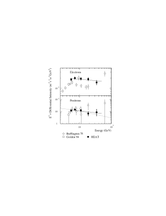
Figure 14: Absolute differential energy spectra for electrons and positrons; the dotted line is a prediction from Strong et al. 1997, and the solid lines are power-law fits to the HEAT results

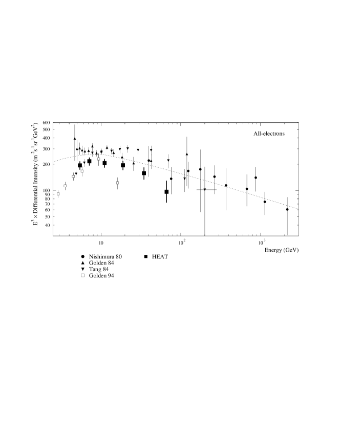
Figure 15: Absolute differential energy spectrum for all electrons $({\rm e^{+}+e^{-}})$; the dotted line is a parametrization from Strong et al. 1997

The absolute differential intensities of electrons and positrons are obtained from equation (1) using Table 1, which lists the number of particles counted in each energy interval $\Delta N$, Table 1 which tabulates the acceptances $\epsilon$ $\!\Omega A$, live time $\Delta t$ and average ToA energy correction factor $f_{ToA}$, as well as $\bar{E}$ and $\Delta E$ (computed with $\alpha=3.1$), and Table 1 which gives the atmospheric contribution. All of the statistical uncertainties associated with these quantities are also contained in these tables. The electron, positron, and all-electron differential intensities are listed in Table 1. The uncertainties are statistical, computed by adding in quadrature all of the contributing uncertainties. The results are plotted in Figures 14 and 15, scaled by $E^{3}$ for clarity, together with other measurements of electron and positron energy spectra ([Buffington et al. 1975, Nishimura et al. 1980, Golden et al. 1984, Tang 1984, Golden et al. 1994]).

abs_flux

fig14

fig15

Besides the uncertainty in determining the instrumental efficiencies discussed in Section 5.1, there are two additional sources of systematic errors. First, the necessity of applying an energy-shift correction to ensure agreement with the momentum indicates a systematic uncertainty in the absolute energy calibration of a few percent, which translates into a $\sim$10% uncertainty in the overall intensity normalization due to the $\alpha=3.1$ power law of the spectrum. Second, uncertainties in the normalization of the proton spectrum translate into a $\sim 25\%$ systematic uncertainty in simulated atmospheric secondary intensities; this has a 0.5% effect on the electron and all-electron intensities, but results in 10% shifts in the positron intensity normalization. Thus, the estimated systematic uncertainty from these sources is 10% for the electron and all-electron intensities, and 14% for the positron intensity.

In Figure 14, we compare our results with previous measurements for which absolute intensities have been given for positrons and electrons separately. We find that the energy spectrum of positrons reported by [Buffington et al. 1975] and [Golden et al. 1994] is generally consistent with our data, although our results show much improved statistical error limits and permit a better estimate of the slope of the energy spectrum. The intensity of positrons of interstellar secondary origin can be calculated, provided the spectrum of parent protons is known, and the parameters of galactic propagation are specified. Such a calculation has been done by [Protheroe 1982], and, more recently, by [Strong, Moskalenko & Schönfelder 1997]. We show in Figure 14 the results of Strong et al. 1997 as a dotted line, and notice the good agreement with our data. In Figure 15, we compare the all-electron energy spectrum ${\rm(e^{+}+e^{-})}$ derived from our data with previous results, also including measurements which did not employ a magnet spectrometer for charge separation. We arbitrarily chose to include only results published since 1980. The dotted line represents a parametrization of the all-electron spectrum used by Strong et al. 1997. We find that all results exhibit similar spectral slopes over the energy range of concern, but that our overall intensity is lower than the average of the previous investigations by about 35%. There are two possible contributors to this systematic discrepancy. First, the absolute energy calibration for the experiments is likely to be uncertain by about 10%, leading to a possible systematic uncertainty in the intensity of the order of 20%. Second, the assessment of the absolute detection efficiency of the instrument is notoriously difficult for all such detectors. Its determination does involve some intuitive judgment, although the more recent investigations, such as ours, benefit in this respect from more sophisticated Monte Carlo simulations than were previously available.

pow_fit

The individual spectral indices for positrons and electrons are $\alpha=3.3\pm 0.2$ and $3.09\pm 0.08$, respectively, over the energy range 5.0 to 50 GeV, as indicated in Table 1 and represented by solid lines in Figure 14. Thus, the positron spectrum appears to be slightly steeper than that of electrons. If all positrons are of interstellar secondary origin, one should expect that radiative energy losses eventually lead to a power-law index that is larger by unity than that of the production spectrum, which follows the ambient spectrum of the parent nuclei, i.e., $\alpha\approx 3.7$ for nuclear spectra of the form $E^{-2.7}$. The spectrum of electrons, on the other hand, should steepen less strongly, to a final slope with $\alpha\approx 3.1$ if electrons are mostly produced at the same primary sources as nuclei, and with the same source spectrum characterized by $\alpha\approx 2.1$. However, these final spectral slopes may not be reached in the energy region below $\sim 100$ GeV. Thus, it would seem proper to fit our data not to a single power law but rather to a spectral form that reflects a transition from the source spectrum (modified by solar modulation) to a spectrum that is fully steepened due to radiative energy losses. Such an analysis had previously been performed on the all-electron spectrum by [Prince 1979] and [Tang 1984]. Here we will not entertain this analysis for our data, as we soon should be able to improve the statistical quality of the results through the inclusion of data from an additional balloon flight. Qualitatively, we may just conclude that the slightly steeper spectrum of positrons, as compared to that of electrons, is to be expected if positrons are predominantly secondary particles. This conclusion must be confirmed by additional data and by an extension of the measurement over a wider energy range.

As mentioned above, a comparison with the calculations of [Protheroe 1982] and Strong et al. 1997 indicates also that the absolute intensity of positrons is close to what may be expected if indeed all positrons are generated subsequent to nuclear interactions in the interstellar medium. More detail on the relative origin of electrons and positrons, and limits on the possible primary contribution to the positron flux, can be obtained if the relative intensity of positrons, i.e., the positron fraction ${\rm e^{+}/(e^{+}+e^{-})}$ (which does not depend on the absolute efficiency of the detector), is investigated as a function of energy. We have presented the results of such an investigation in previous papers ([Barwick et al. 1995, Barwick et al. 1997a]).

The results described in this paper have been obtained with the first balloon flight of the HEAT spectrometer. We believe that the high level of hadronic background rejection achieved with this instrument has led to data of high quality, limited only by the statistical uncertainties of a single balloon flight. A second balloon flight which has been carried out successfully from Lynn Lake, Manitoba in 1995 August, covers the energy range from $\sim 1$ GeV upwards. The analysis of the combined data set is presently in progress, and results will soon be reported.

Table 1: Data selection criteria

Cleanliness requirements

DTH filter algorithm passed

DTH rigidity reconstruction algorithm passed

$N\!B\geq 9$ (Number of tubes in DTH bending view used in fit)

$N\!N\!B\geq 4$ (Number of tubes in DTH non-bending view used in fit)

$\chi^{2}<10$ (DTH rigidity goodness of fit)

$D\!E\!V\!\_X<0.080$ cm (Average residual in $X$ (non-bending) projection)

$D\!E\!V\!\_Y<0.014$ cm (Average residual in $Y$ (bending) projection)

$D\!E\!V\!\_Z<0.020$ cm (Average residual in $Z$ (vertical) projection)

$\int\!B\,dl>2.2$ kG m (Integrated B-field over the track length)

$M\!\!D\!R>60$ GV

$M\!\!D\!R/\left|R\right|>4$

$\left|E/p\right|<3.0$

$0.70<\beta<1.65$ (Velocity range, downward-going)

$\left|T\!O\!F\!\_X-D\!T\!\_X\right|<20$ cm (Agreement between DTH track and TOF timing)

Propagated DTH track traverses both TOF and EC

Propagated DTH track traverses $\geq 4$ TRD chambers

Electron selection criteria

$0.68<Z<1.45$ (Charge)

EC starting depth $t<0.89$ radiation lengths

$\chi^{2}<2.6$ (EC goodness of fit)

$\log_{10}\left[(L_{ep}^{PHA}-\sigma_{L_{ep}^{PHA}})\cdot(L_{ep}^{TS}-\sigma_{L_{ep}^{TS}})\right]>3$ (TRD likelihood ratio)

Interacting proton selection criteria

Same as electron selection criteria except:

$\log_{10}\left[(L_{ep}^{PHA}+\sigma_{L_{ep}^{PHA}})\cdot(L_{ep}^{TS}+\sigma_{L_{ep}^{TS}})\right]<-1$ (TRD likelihood ratio)

cccc Raw numbers of electrons 0pt $E_{ToA}$ (GeV) & # Electrons $\Delta N_{\rm e^{-}}$ # Positrons $\Delta N_{\rm e^{+}}$ # All-electrons $\Delta N_{\rm e}$ 5.0 – 6.0 & $1231\pm 36$ $107\pm 11$ $1338\pm 37$
6.0 – 8.9 $1781\pm 43$ $161\pm 14$ $1942\pm 45$
8.9 – 14.8 $918\pm 31$ $75^{+10}_{-9}$ $993\pm 33$
14.8 – 26.5 $340\pm 20$ $18.5^{+5.8}_{-3.9}$ $359\pm 20$
26.5 – 50.0 $75^{+10}_{-9}$ $6.1^{+3.7}_{-2.1}$ $81^{+10}_{-9}$
50.0 – 100.0 $19.2^{+5.7}_{-4.0}$

ccccc Energy intervals and effective acceptances the live time is $\Delta t=(18.043\pm 0.036)$ hr, and the average ToA energy correction factor is $f_{ToA}=(1.086\pm 0.020)$ 0pt $E_{ToA}$ (GeV) & $\bar{E}$ (GeV) $\Delta E$ (GeV) $\epsilon$ $\!\Omega A\>(\mbox{cm}^{2}\,\mbox{sr})$ 5.0 – 6.0 & 5.45 0.991 $181\pm 18$
6.0 – 8.9 7.16 2.78 $193\pm 19$
8.9 – 14.8 11.1 5.50 $194\pm 20$
14.8 – 26.5 18.9 10.7 $189\pm 19$
26.5 – 50.0 34.5 21.1 $160\pm 16$
50.0 – 100.0 66.4 44.0 $207\pm 21$

ccc Atmospheric secondary electron and positron intensities at 5.7 g/cm² 0pt $E_{ToA}$ (GeV) & $j_{sec}^{-}\!({\mbox{m}}^{2}\,\mbox{s}\,\mbox{sr}\,\mbox{GeV})^{-1}$ $j_{sec}^{+}\!({\mbox{m}}^{2}\,\mbox{s}\,\mbox{sr}\,\mbox{GeV})^{-1}$ 5.0 – 6.0 & $(1.8\pm 0.6)\times 10^{-2}$ $(2.4\pm 0.6)\times 10^{-2}$
6.0 – 8.9 $(7.6\pm 2.3)\times 10^{-3}$ $(9.7\pm 2.2)\times 10^{-3}$
8.9 – 14.8 $(2.1\pm 0.6)\times 10^{-3}$ $(2.5\pm 0.7)\times 10^{-3}$
14.8 – 26.5 $(4\pm 1)\times 10^{-4}$ $(5.3\pm 1.1)\times 10^{-4}$
26.5 – 50.0 $(7\pm 2)\times 10^{-5}$ $(9\pm 2)\times 10^{-5}$
50.0 – 100.0 $(1.1\pm 0.7)\times 10^{-5}$ $(1.2\pm 0.7)\times 10^{-5}$

ccc Secondary-to-primary electron ratios at 6 g/cm² 0pt Energy (GeV) & MC sec./pri. HEAT sec./pri. 4.5 – 6.0 & 0.04 $\pm$ 0.01 0.04 $\pm$ 0.03
6.0 – 8.9 0.04 $\pm$ 0.01 0.04 $\pm$ 0.03
8.9 – 14.8 0.04 $\pm$ 0.01 0.01 $\pm$ 0.03
14.8 – 25.6 0.05 $\pm$ 0.01 0.01 $\pm$ 0.03
25.6 – 50.0 0.06 $\pm$ 0.02

clll Differential intensities of electrons, in $({\mbox{\rm m}}^{2}\,\mbox{\rm s}\,\mbox{\rm sr}\,\mbox{\rm GeV})^{-1}$ 0pt $\bar{E}$ (GeV) & $j_{pri}^{-}(\bar{E})$ $j_{pri}^{+}(\bar{E})$ $j_{pri}^{\pm}(\bar{E})$ 5.45 & $1.13\pm 0.12$ $0.076\pm 0.016$ $1.20\pm 0.13$
7.16 $0.548\pm 0.057$ $0.0405\pm 0.0070$ $0.589\pm 0.062$
11.1 $0.141\pm 0.016$ $(9.2^{+2.1}_{-2.0})\times 10^{-3}$ $0.151\pm 0.017$
18.9 $0.0278\pm 0.0033$ $(1.00^{+0.52}_{-0.38})\times 10^{-3}$ $0.0288\pm 0.0035$
34.5 $(3.64^{+0.62}_{-0.58})\times 10^{-3}$ $(2.1^{+1.9}_{-1.1})\times 10^{-4}$ $(3.84^{+0.64}_{-0.60})\times 10^{-3}$
66.4 $(3.30^{+1.11}_{-0.83})\times 10^{-4}$

ccc Power-law fits to the differential spectra 0pt $J_{\circ}E^{-\alpha}$ & $\alpha$ $J_{\circ}\>(\mbox{GeV}^{-1}\,\mbox{m}^{-2}\,\mbox{s}^{-1}\,\mbox{sr})$ Electrons & $3.086\pm 0.081$ $227\pm 45$
Positrons $3.31\pm 0.23$ $24\pm 12$

Figure 1: Altitude profile of the 1994 balloon flight

Figure 2: HEAT instrument schematic cross-section

Figure 3: TOF $\beta$ and charge distributions

Figure 5: TRD proton and electron efficiencies

Figure 6: TRD likelihood ratio $L_{\mbox{\scriptsize\it Total}}$ distribution for protons and electrons

Figure 7: Distribution of DTH residuals for bending-view tubes

Figure 8: DTH residuals as a function of tube radius for bending-view tubes

Figure 9: MDR distribution for electron events

Figure 10: EC energy distribution for 10 GeV MC events

Figure 11: EC proton and electron efficiencies

Figure 12: $E/p$ distributions for electrons and positrons

Figure 13: Positron fraction as a function of atmospheric depth