IMAPS Observations of Interstellar Neutral Argon and the Implications for Partially Ionized Gas

Abstract

We use the absorption features from the resonance transitions of neutral argon at 1048 and 1066 Å to determine interstellar argon abundances or their lower limits toward nine early-type stars. These features were observed with the Interstellar Medium Absorption Profile Spectrograph (IMAPS) along sight lines with low reddening and low fractional abundances of molecular hydrogen. Four of the sight lines in our sample have reliably measured interstellar Ar abundances, of which three also have good determinations of $N({\rm H~{}I})$. We find that the interstellar Ar is below its solar and B-star abundance with respect to hydrogen toward $\zeta$ Pup, $\gamma^{2}$ Vel and $\beta$ Cen A with (logarithmic) reduction factors $D=-0.37\pm 0.09\,{\rm dex}$, $D=-0.18\pm 0.10\,{\rm dex}$, and $D=-0.61\pm 0.12\,{\rm dex}$, respectively.

While Ar can condense onto the surfaces of dust grains in the interiors of dense clouds, it is unlikely that argon atoms are depleted by this process in the low-density lines of sight considered in this study. Instead, we propose that the relatively large photoionization cross section of Ar makes it much easier to hide in its ionized form than H. In regions that are about half ionized, this effect can lower Ar I/H I by $-0.11$ to $-0.96\,{\rm dex}$, depending on the energy of the photoionizing radiation and its intensity divided by the local electron density. We apply this interpretation for the condition of the gas in front of $\beta$ Cen A, which shows the largest deficiency of Ar. Also, we determine the expected magnitudes of the differential ionizations for He, N, O, Ne and Ar in the partly ionized, warm gas in the local cloud around our solar system. For the local cloud and others that can be probed by UV studies, the observed Ar I to H I ratio may be a good discriminant between two possible alternatives, collisional ionization or photoionization, for explaining the existence of partly ionized regions.

1 Introduction

For diffuse, neutral gases in space, two fundamental processes influence the pattern of abundances of different elements in free atomic form: (1) the contributions from various nucleosynthetic sources and how the outcomes are influenced by mixing and transport processes, and (2) the removal of atoms as they are incorporated into dust grains. There have been numerous studies of the gas-phase abundances of elements in the local region of our Galaxy (Cowie & Songaila 1986; Savage & Sembach 1996), using information provided by UV interstellar absorption lines in the spectra of stars. These investigations have generally focused on the second of the two processes (Jenkins, Savage, & Spitzer 1986; Sofia, Cardelli, & Savage 1994), using abundances in the Sun or nearby, early-type stars as a comparison template for material that would be free of dust. By contrast, studies of very distant gas systems that produce absorption lines in quasars have concentrated on the history of element production (Pettini, Boksenberg, & Hunstead 1990; Pettini et al. 1994, 1997; Timmes, Lauroesch, & Truran 1995; Lu et al. 1996), i.e., its character and rate, and have regarded the depletions caused by dust formation as a possible complication that, if present, must be compensated for.

It is generally recognized that the overall severity of a given element’s depletion is correlated with the stability of chemical bonds of likely compounds in the grains. This differential effect can be interpreted to result from either the relative completeness of the element’s incorporation into grains in the outer envelopes of stellar atmospheres (Field 1974), how rapidly the element contributes to the growth of grains in dense interstellar clouds (Snow 1975; Tielens & Allamandola 1987), or the relative resistance of different grain components due to destruction by interstellar shocks (Seab 1987; Jones et al. 1994; Tielens et al. 1994). Elements that have very strong bonds in dust compounds, such as Al, Ti and Ca, are depleted by as much as 2 to 3 orders of magnitude (Jenkins 1987), while more volatile elements, such as C, N and O, have depletions of only factors of 2 or 3 (Hibbert, Dufton, & Keenan 1985; Meyer, et al. 1994; Cardelli et al. 1996; Meyer, Cardelli, & Sofia 1997; Meyer, Jura, & Cardelli 1997) or perhaps even less – see below. Noble gases represent the greatest extreme of volatility, since they generally do not form chemical bonds with solid compounds, and they can adhere to grains only through the very weak van der Waals force (Watson 1976). This paper presents observations of the interstellar abundances of one such noble gas, the element argon in its neutral form. One feature of this study is the fact that the lines of sight have a low average gas density, and this further reduces the likelihood that the abundances are modified by dust formation (Jenkins 1987).

Neutral argon has two strong resonance lines in the far ultraviolet. Their f-values differ by a factor of 4 (Federman et al. 1992), which allows one to test for line saturation and apply corrective measures (or realize that the saturation is hopelessly bad). While the interstellar Ar features are easily recognizable in most spectra, their great strength turns out to be a liability because the lines become strongly saturated when dense clouds are being investigated. For instance, for a velocity dispersion $b$ = $10\,{\rm km~{}s}^{-1}$ and $N({\rm H})=10^{20}{\rm cm}^{-2}$, the weaker of the two Ar I lines at 1066.66 Å would have a central optical depth $\tau_{0}=4$ if the argon had a cosmic abundance ratio with respect to hydrogen. The consequences of such saturation are lessened if the line’s velocity structure is mostly resolved by the instrument, because one can interpret the apparent optical depth as a function of velocity (Savage & Sembach 1991; Jenkins 1996) instead of the much cruder approach of just measuring the equivalent widths and using the standard curve of growth to derive a total column density. The observations reported here take advantage of an instrument that can, in most circumstances, resolve nearly all of the velocity detail of a feature, which puts us in a better position to derive accurate column densities than was possible with the Copernicus satellite (Rogerson et al. 1973a).

The reference abundance of Ar derived for the Sun or B stars is now understood with reasonable accuracy (see §4), and the difference between the two is not very large. The only major uncertainty is whether or not the solar or B-star abundances are indeed appropriate standards for comparison. Recently accumulated evidence (Cardelli et al. 1996; Fitzpatrick 1996; Meyer, Cardelli, & Sofia 1997; Meyer, Jura, & Cardelli 1997; Sofia et al. 1997) indicates that some mildly depleted elements do not follow the usual trend of depletions becoming stronger in denser interstellar clouds (Spitzer 1985; Jenkins, Savage, & Spitzer 1986; Jenkins 1987), as we would expect if these elements were major constituents in grains that are more abundant and larger in dense regions because they are protected from interstellar shocks and are allowed to grow rapidly (Tielens & Allamandola 1987; Jenkins 1989). This phenomenon has raised the possibility that the intrinsic abundances of heavier elements in the local interstellar medium (in both solid and gaseous form) may be lower than for the nearby stars, and that the depletions by grain formation for some of them are relatively small in comparison to this deficiency.

A noteworthy property of argon is that, while its neutral form has an ionization potential greater than that of hydrogen, its cross section for photoionization above this threshold is extraordinarily high. This is of no consequence for an interstellar cloud that is thick enough to have virtually all of its interior shielded from outside sources of ionizing radiation by a large column of neutral hydrogen. However the situation for thinner clouds is different. Since the absorption cross section of hydrogen diminishes for energies well above the Lyman limit, we naturally expect that relatively hard radiation must penetrate the cloud and partially ionize the hydrogen and argon atoms. In circumstances where some or almost all of the hydrogen is ionized, the fraction of argon that remains in neutral form can be considerably lower than the corresponding fraction for hydrogen. As a result, this element may deceptively appear to be “depleted” relative to hydrogen if one makes the simple-minded assumption that both elements are predominantly neutral. We will explore this issue in more detail in §6.2 and present an assessment of the conditions where this effect is likely to be significant.

Our discussion starts with the observations and data reduction in §2, followed by the resulting Ar I column densities (§3) and how they relate to measurements of neutral hydrogen along the same lines of sight (§4). In §5 we briefly compare our results with those of previous observations at much lower resolution. On the theoretical side, in §6.1 we will present in greater depth the arguments that support our assertion that the apparent deficiencies of Ar I relative to H I are unlikely to be caused by the depletion of Ar onto dust grains. We argue in §6.2 that for our observing circumstances the most likely reason for a reduction in Ar I is because it is readily photoionized by energetic radiation that is able to penetrate the region. We can use this effect to understand better the nature of the partially ionized clouds. Ar is a good tracer element to indicate how strongly the apparent abundances of other elements could be influenced by ionization, and this information is crucial for research on the chemical evolution of the gases in different contexts.

2 Observations & Data Reduction

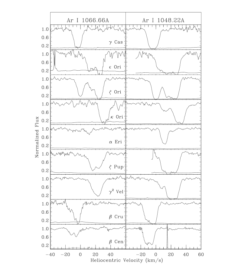
The ultraviolet absorption line data used for this study were obtained with the Interstellar Medium Absorption Profile Spectrograph (IMAPS) during the first ORFEUS-SPAS Space Shuttle mission in September 1993. IMAPS is a simple, objective-grating echelle spectrograph that can record the spectrum of a bright, hot star in the wavelength interval 950 to 1150 Å, a spectral region that is densely populated with atomic and molecular transitions from the neutral and ionized interstellar medium (ISM) (Morton 1975; Spitzer & Jenkins 1975; Cowie & Songaila 1986). The instrument was designed to achieve the high resolving power needed to show most of the detailed velocity structures in the ISM. Jenkins, et al. (1996) give a comprehensive description of the IMAPS instrument, its flight on the first ORFEUS-SPAS mission, and the methods of data correction and analysis. This paper includes observations in 9 sight lines for which the neutral argon resonance transitions at 1048.220 and 1066.660 Å were recorded. These paths through the ISM are toward nearby, early-type stars with low reddening. Table 1 shows the list of target stars with their galactic coordinates, spectral types, visual magnitudes, distances, B$-$V color excesses, and line-of-sight fractions of molecular hydrogen.

Table 1: Interstellar Sight Lines

Star	l	b	Type	V	Distance	E(B$-$V)	Log f(H2)
$\gamma$ Cas	123.58	$-$2.15	B0 IVe	2.47	188	0.13	$-$5.50
$\epsilon$ Ori	205.22	$-$17.24	B0 Iae	1.70	412	0.05	$-$3.91
$\zeta$ Ori	206.46	$-$16.59	O9.5 Ibe	2.05	251	0.05	$-$4.66
$\kappa$ Ori	214.52	$-$18.50	B0.5 Iav	2.06	221	0.04	$-$4.92
$\alpha$ Eri	290.84	$-$58.79	B3 Vpe	0.46	44	0.07	…
$\zeta$ Pup	255.98	$-$4.71	O5 Iaf	2.25	429	0.04	$-$5.50
$\gamma^{2}$ Vel	262.81	$-$7.70	WC8+O7.5e	1.78	258	0.05	$-$5.51
$\beta$ Cru	302.47	3.18	B0.5 III	1.25	108	0.03	…
$\beta$ Cen A	311.77	1.25	B1 III	0.61	161	0.02	$-$6.44

Once the images of the echelle spectra have been reduced and appropriately coadded, the fluxes vs. wavelength must be extracted. Our basic extraction method was discussed in Jenkins et al. (1996), however we have altered some of the procedures since the time of that article. Jenkins et al. described a spectral extraction slit that had a uniform cross-dispersion shape and spacing between orders. These parameters are important for the extraction because the low intensity wings of adjacent echelle orders overlap in the cross-dispersion direction. We used extraction slits with predefined empirically determined cross-dispersion profile shapes which varied slightly as a function of spectral order. We also allowed the profile to be broadened or narrowed, and the distance between the orders could vary slightly in order to better fit the data. These modifications to the extraction slit were performed interactively during the extraction.

Our background level determination for the extraction procedure also differed from that discussed in Jenkins et al. (1996). Here we examined the regions which contain the least contribution from the spectral orders, halfway between the order being extracted and each of the adjacent orders. Since the shape of the order’s cross-dispersion profile is known, we are able to subtract the contributions of the 2 adjacent orders from each of these interorder regions. The remaining light was assumed to be the smooth background which changes with position in the echelle dispersion direction. The average of the two interorder points on either side of the order being extracted was used as the background level and subtracted. To test the reliability of this method, we inspected the cores of lines that, from their appearance, are likely to be fully saturated and hence have zero intensity in their cores. We found that the rms dispersion of these zero levels was approximately 5% of the local continuum flux level. Figure 1 shows the extracted, normalized profiles of Ar I $\lambda\lambda$ 1048 and 1066 Å toward the stars in our sample. The sampling interval for the curves in Figure 1 is one half-pixel on the CCD since the data are put into an oversampled format for reduction purposes (Jenkins et al. 1996).

Figure 1: Normalized flux versus velocity for the $\lambda\lambda$ 1048, 1066 Å transitions of neutral Ar in the interstellar medium toward our sample of stars. The lower curve in each frame represents the 2$\sigma$ statistical error in the data.

An interesting exercise is to compare the IMAPS absorption profiles with the corresponding ones observed in the 1970’s with Copernicus (Rogerson et al. 1973a). Although these two instruments had very different wavelength resolving powers (Copernicus could resolve a velocity difference of about $15\,{\rm km~{}s}^{-1}$ compared to $4\,{\rm km~{}s}^{-1}$ for IMAPS), the equivalent widths of the absorption lines should be the same if the correct continua and background corrections were assigned in each case. Table 2 shows the equivalent width measurements for the three N I transitions near $\lambda$ 1134 Å and the two Ar I transitions at $\lambda$ 1048 Å and $\lambda$ 1066 Å for $\gamma^{2}$ Vel (Morton & Bhavsar 1979), $\zeta$ Pup (Morton 1978) and $\epsilon$ Ori (Shull 1979). In the cases where the absorption features reach near zero intensity (all of the N I and Ar I $\lambda$ 1048 Å features, as well as Ar I $\lambda$ 1066 Å toward $\epsilon$ Ori), the IMAPS equivalent widths agree well ($<$ 10% difference) with those from Copernicus. However the lines which do not approach zero intensity, i.e. the weaker line of Ar I ($\lambda$ 1066 Å) toward $\zeta$ Pup and $\gamma^{2}$ Vel, show substantial differences ($>$ 10%) when comparisons are made between the IMAPS and Copernicus measurements. Background levels were often difficult to determine for Copernicus data, and we have no reason to believe that the IMAPS background determinations for the Ar I line at 1066 Å are worse than for any other region of the spectrum. We therefore believe that our background determinations may be more accurate for these weak lines than those determined for Copernicus in this spectral region.

Table 2: IMAPS vs Copernicus Equivalent Width Measurements

		Wλ (mÅ)
Star	Instrument	Ar I $\lambda$ 1048.2	Ar I $\lambda$ 1066.6	N I $\lambda$ 1134.1	N I $\lambda$ 1134.4	N I $\lambda$ 1134.9
$\epsilon$ Ori	IMAPS	112	76	128	137	141
	Copernicus	106	78	126	136	152
$\zeta$ Pup	IMAPS	88	53	112	120	128
	Copernicus	89	65	114	123	131
$\gamma^{2}$ Vel	IMAPS	78	41	92	118	118
	Copernicus	72	54	99	113	107

Jenkins & Peimbert (1996) analyzed the telluric excited O I lines that appeared in the IMAPS spectrum of $\zeta$ Ori A, in order to determine the width of the instrument’s profile. Assuming that the lines are thermally broadened for $T$ = 1000 K, they found that the instrumental smearing function for those observations was approximately a 3.5 pixel (FWHM) Gaussian, a width that corresponds to a Doppler shift of 4 km s^-1. It is reasonable to assume that the resolving power for the other stars observed during the ORFEUS-SPAS-I mission is approximately the same as that for $\zeta$ Ori A. It is lower than what should have been achievable in principle with IMAPS and the pointing stability of the spacecraft. We attribute the degradation to the relief of mechanical stresses within a sticky bearing that supported the echelle grating. This problem led to small motions of the spectrum while the exposures were underway. The magnitude and character of this effect has been discussed in detail by Jenkins, et al. (1996).

3 Column Densities of Argon

3.1 Method of Analysis

An important advantage of having observations that can resolve much of the velocity structure is the ability to more explicitly detect and possibly correct for line saturation. In addition, sections of the profile at different velocities may exhibit interesting behavior that would otherwise be lost at low resolution. While we could have used our observations to define some combination of separate components and then determined their amplitudes, velocity centroids and widths that are most consistent with the data, we instead have chosen a more generalized procedure. We measured the intensity $I(v)$ in terms of the continuum level $I_{0}$ and derived an apparent optical depth as a function of velocity,

$$\tau_{a}(v)=\ln\Bigl{(}{I_{0}\over I(v)}\Bigr{)}~{},$$ (1)

a function whose interpretation has been described in some detail by Savage & Sembach (1991) and Jenkins (1996). For the ideal cases where either the line is very weak or we are sure that the instrument has resolved the finest details in velocity, $\tau_{a}(v)$ gives an accurate depiction of a differential column density per unit velocity through the relation

$$N_{a}(v)=3.768\times 10^{14}{\tau_{a}(v)\over f\lambda}~{}{\rm cm}^{-2}({\rm km~{}s}^{-1})^{-1}~{},$$ (2)

where $f$ is the transition’s $f$-value and $\lambda$ is expressed in Å.

In some circumstances, $N_{a}(v)$ derived through the use of Eqs. 1 and 2 can give an underestimate for the true column density per unit velocity $N(v)$. If narrow, saturated structures within the velocity profile are smoothed over by the instrument, one will not fully recognize how closely the cores of the features approached the zero intensity level before the smoothing took place, thus leading to an incorrect representation of $N(v)$. Fortunately, we can sense when this is happening (and over what velocity range) if we are able to observe two or more lines with different $f$-values and note that the weaker line gives a larger $N_{a}(v)$ than corresponding values for the stronger line. Jenkins (1996) has described how one can use this information to derive a good approximation to the true $N(v)$, aside from the fact that it has been smoothed. This method relies on a point-by-point correction technique that mirrors the classical curve of growth analysis method that has been used for the equivalent widths of lines.

A proper application of the $\tau_{a}(v)$ correction procedure requires that the velocity scales of the strong and weak lines are accurately matched. In their IMAPS spectrum that showed many features of H₂ in the spectrum of $\zeta$ Ori A, Jenkins & Peimbert (1996) found that the velocities were internally consistent to within an rms dispersion of only $0.5\,{\rm km~{}s}^{-1}$. Since our method of correcting for image distortions and deriving the wavelength scales is identical to that of Jenkins & Peimbert, we expect a similar accuracy in this study.

Beyond the considerations discussed above, other key factors that influence the accuracy of the column densities include a good knowledge of the background and continuum levels in the region of the absorption and, of course, accurate oscillator strengths for the transitions being measured. We have already discussed in §2 the probable accuracy of our background subtractions. The stellar continua over the velocity breadth of the absorption features are quite smooth and well determined for all of the stars. We found that a third-order polynomial fitted to the spectrum adjacent to the absorption gave a satisfactory definition of the continuum. We estimate the continuum fitting error to be 0.35 times the rms deviation of the data about the fitted continuum in the spectral region adjacent to the absorption line of interest [see Savage, Cardelli & Sofia (1992) for a justification of this error estimate]. For the two Ar transitions we used the oscillator strengths $f_{1048}=0.257\pm 0.013$ and $f_{1066}=0.064\pm 0.003$ reported by Federman et al. (1992).

3.2 Results

The optical depth correction procedure discussed in §3.1 was applied to the Ar lines toward the stars in our sample. Valid corrections can not be made for line pairs in regions where the weaker line has near zero intensity. Figure 2 shows the logarithmic column densities as a function of velocity for the four sight lines with corrected optical depth profiles which we believe do not contain any uncertain points ($\zeta$ Pup, $\gamma^{2}$ Vel, $\beta$ Cen A and $\alpha$ Eri); the remaining five sets of profiles could not be corrected across the entire velocity extent of the Ar absorption. Integrating Eq. 2 over the velocity extent of the Ar absorption yields the column densities and limits listed in Table 3. The column densities were derived using the corrected optical depth profiles, and the limits are based on the uncorrected $\lambda$1066 Å optical depths. The reported uncertainties are based on the statistical errors in the data, the uncertainty in the oscillator strengths, the error in continuum definition, and a background uncertainty of 5% of the continuum flux level, all of which were added in quadrature. No uncertainty relating to the correction of the optical depth profiles is included. The differences between the column densities measured after and before the optical depth correction was applied to the weaker line are also shown in the third column of Table 3 for those lines which could be corrected. The differences between the pre- and post-correction column densities are quite small for these sight lines, all within the 1-$\sigma$ measurement errors. This agreement gives us added confidence that our background determinations are probably reliable.

Figure 2: Logarithmic column densities $N(v)$ (see Eq. 2) as a function of velocity toward $\zeta$ pup, $\gamma^{2}$ Vel, $\beta$ Cen A and $\alpha$ Eri. The $\pm 1\sigma$ error bars include statistical, continuum fitting and background uncertainties. The optical depths on the right-hand side are representative of the $\lambda$ 1066 Å Ar I transition. The ⊕ symbol with an arrow in each frame indicates the location of possible telluric Ar contamination.

Table 3: Integrated Argon Gas-Phase Abundances and Depletions

Star	Log N(Ar I)	Log N(Ar I) $-$ Log Na(Ar I)	Log[ N(H I) + 2N(H2)]	D
$\gamma$ Cas	$>$14.10	…	20.16$\pm$0.05	$>-$0.58
$\epsilon$ Ori	$>$14.39	…	20.46$\pm$0.06	$>-$0.59
$\zeta$ Ori	$>$14.44	…	20.40$\pm$0.06	$>-$0.48
$\kappa$ Ori	$>$14.18	…	20.54$\pm$0.04	$>-$0.88
$\alpha$ Eri	13.19 $\pm$ 0.09	0.00	$<$19.36	$>-$0.69
$\zeta$ Pup	14.14 $\pm$ 0.08	0.03	19.99 $\pm$ 0.02	$-$0.37 $\pm$ 0.09
$\gamma^{2}$ Vel	14.11 $\pm$ 0.08	0.08	19.77 $\pm$ 0.03	$-$0.18 $\pm$ 0.10
$\beta$ Cru	$>$14.10	…	…	…
$\beta$ Cen A	13.45 $\pm$ 0.10	0.00	19.54 $\pm$ 0.06	$-$0.61 $\pm$ 0.12

4 Relative Abundances of Neutral Argon

In order to study the significance of our argon measurements, we must compare them to measurements of other elements in the same gas. When possible, hydrogen is generally used as the comparison species. The cosmic abundance ratio of Ar to H is well determined. Anders & Grevesse (1989) give a logarithmic abundance for Ar/H of $-$5.44 $\pm$ 0.10 which is based on corrected solar measurements, H I and H II regions, and stars. Since our objective is to study the abundances of Ar in the ISM, it would not be appropriate to use a cosmic abundance which includes interstellar values. Keenan et al. (1990) and Holmgren et al. (1990) find logarithmic ratios of $-$5.50 and $-$5.51 for Ar/H in B star photospheres with uncertainties of $\pm$ 0.05 and $\pm$ 0.10 respectively. Solar photospheric abundances determined from correcting solar coronal observations have produced logarithmic ratios of $-$5.46 $\pm$ 0.1 (Anders & Grevesse 1989) and $-$5.45 $\pm$ 0.08 (Meyer, 1989). We have taken the weighted average of these B star and solar ratios to get a logarithmic cosmic abundance ratio of $-$5.48 $\pm$ 0.04 for argon to hydrogen.

The expected dominant ionization state for argon in most neutral hydrogen regions is Ar I since the ionization potential for neutral Ar is 15.76 eV compared to 13.59 eV for H. Making the plausible initial assumption that all of the argon associated with neutral H is Ar I (an assumption that must eventually be withdrawn, as discussed in §6.2), we determine the reduction of Ar in the gas phase below its expected ratio to hydrogen through the relation

$$D=\log\left(\frac{N({\rm Ar~{}I})}{N({\rm H~{}I})+2N({\rm H_{2}})}\right)_{observed}-\log\left(\frac{{\rm Ar}}{{\rm H}}\right)_{cosmic}.$$ (3)

Table 1 shows that the H₂ column densities toward the stars in our sample are very small compared to H I and can therefore be neglected. The interstellar neutral hydrogen column densities toward $\gamma^{2}$ Vel and $\zeta$ Pup are $10^{19.77\pm 0.03}$ and $10^{19.99\pm 0.02}\,{\rm cm}^{-2}$, respectively, from a weighted average of the Bohlin, Savage & Drake (1978) and Diplas & Savage (1994) values. We adopt the determination $N({\rm H})=10^{19.54\pm 0.06}\,{\rm cm}^{-2}$ toward $\beta$ Cen A from Rogerson & York (1973). A reliable neutral hydrogen column density is not available toward $\alpha$ Eri because the stellar H absorption badly contaminates the interstellar H spectral features. For this sight line we estimate a total H (i.e. 2H₂ + H I + H II) column density from the S II column density; with an ionization potential of 23.33 eV, the S II ion resides in both the neutral and the ionized ISM toward $\alpha$ Eri. Assuming that S is undepleted (Fitzpatrick & Spitzer 1997) and that the cosmic S/H abundance is represented by B stars [Log(S/H) = $-$4.91 (Snow & Witt 1996)], we find that the total logarithmic interstellar hydrogen column density toward $\alpha$ Eri is Log N(H) = 19.36 for the S II column density determined by Rogerson, et al. (1973b). Based on the N I and N II abundances toward $\alpha$ Eri, it is possible that a substantial fraction of the H in the sight line is ionized.

For the three cases with good measurements of N(H I) we determined the apparent logarithmic deficiencies $D$ of argon with respect to hydrogen in the fifth column of Table 3. The accompanying errors include the uncertainty in the Ar I and H I abundance determinations, and the uncertainty in the cosmic Ar-to-H abundance ratio added in quadrature. The uncertain neutral H column density toward $\alpha$ Eri only allows a limit of $D>-0.69$ toward this star. Lower limits for $D$ toward the other stars in our sample are given in Table 3.

Due to the low orbit (295 km) of ASTRO-SPAS, there is a possibility that telluric lines could contribute some additional absorption in our spectra. Neutral argon is an abundant species in the Earth’s atmosphere, so we must know the telluric absorptions’ effects on the interstellar profiles. We calculated the column density of telluric neutral Ar that IMAPS would observe through as a function of zenith angle using the global thermospheric model of Hedin et al. (1974) with input from the measured solar parameters for the observation days (K. Schatten, private communication) and the assumption of a spherical Earth. The expected Ar absorption component in the atmosphere is generally small except for the largest zenith angles, i.e., $N({\rm Ar~{}I})>10^{12}\,{\rm cm}^{-2}$ only when $z>90\arcdeg$. With our computed time-averaged column densities for the target zenith angles of our exposures, we estimate that the values $<10^{11}$, $2\times 10^{12}$, $2\times 10^{11}$ and $6\times 10^{10}$ atoms cm^-2 apply to the telluric contamination of the 1066 Å absorptions toward $\zeta$ Pup, $\gamma^{2}$ Vel, $\beta$ Cen A and $\alpha$ Eri, respectively. These numbers should serve only as an approximate indication of the possible telluric contamination, since the predicted column densities could vary by a factor of 2 in any given day. The heliocentric velocity of the telluric absorption toward each of these stars is shown in Figure 2. Any addition to Ar column densities from telluric lines would tend to make the Ar in a sight line appear less deficient in the ISM than it actually is.

5 Comparison with Previous Results

The Copernics spectrometer was used to observe the neutral interstellar argon lines toward several stars. These earlier results have been summarized by Meyer (1989). Because of the great strength of the absorption features (see §1) and their tendency to saturate for moderately dense lines of sight, these measurements often led to large uncertainties in the Ar abundances. For the very lightly reddened sight lines toward $\zeta$ Pup and $\gamma^{2}$ Vel, Morton (1978) and Morton & Bhavsar (1979) have reported depletions of $-$0.31 $\pm$ 0.3 and $-$0.20 $\pm$ 0.15, for the respective stars based on data fromCopernicus. These are very similar to the logarithmic deficiencies determined in this paper ($-$0.37 $\pm$ 0.09 and $-$0.18 $\pm$ 0.10) even though the original $f$-values (Morton & Smith 1973) and reference abundance (Withbroe 1971) used for the Copernicus determinations have since been revised. It is the accuracy of the IMAPS data, however, that allows us to confidently conclude that the Ar is deficient with respect to our adopted reference abundance in our sample’s sight lines, and that the relative reduction levels are not constant for this element in the ISM.

Federman et al. (1992) argue that the strength of the absorption transitions requires that sight lines with small columns of neutral gas be used to determine reliable interstellar column densities of Ar. Using updated $f$-values and a new reference abundance, they reanalyzed the Copernicus results from the low column density, low reddening sight lines toward $\alpha$ Vir (York & Kinahan 1979) and $\lambda$ Sco (York 1983) and reaffirmed the previous conclusions that Ar/H is not below the solar value for the interstellar medium near the Sun. This seems to conflict with our analysis of low column density, low reddening lines of sight which show that argon is indeed deficient in the neutral ISM in the Sun’s vicinity. The fact that we find varied levels of Ar deficiencies, however, does not rule out such a difference as being valid.

6 Discussion

6.1 Can Ar Deplete onto Dust Grains?

In studies of lightly depleted elements such as O, N and C (Cardelli et al. 1996; Meyer, Cardelli, & Sofia 1997; Meyer, Jura, & Cardelli 1997), the observed $D$ values (about equal to $-$0.37, $-$0.09 and $-$0.39, respectively as compared to solar values) are uniform over vastly different interstellar conditions. Such findings have led to the interpretations that the abundances of these elements are not appreciably affected by the formation of dust grains, at least over the range of cloud thicknesses and internal densities surveyed. Instead, it has been argued that the total abundances of such elements in the local gas may be lower than those of the Sun and possibly B stars (Fitzpatrick 1996). While some of the deficiency of argon that we have detected may likewise be explained partly by this phenomenon, the variation of $D$ shown for the entries for $\zeta$ Pup, $\gamma^{2}$ Vel and $\beta$ Cen A in Table 3 indicates that some additional process must be at work. We explore in this section the plausibility that argon could be depleted by interacting with other materials in the medium.

In the interstellar medium, there are very few gas-phase compounds that incorporate the argon atom, since this element is chemically inert. While Ar can form a stable hydride Ar H⁺, Duley (1980) argues that the concentrations of Ar H⁺ in the interstellar medium should be insignificant. We are thus left to consider only the direct attachment of single argon atoms onto the surfaces of dust grains.

The characteristic e-folding time for the depletion of an element by condensing onto dust grains is given by

$$t_{depl.}=\big{[}\Sigma_{d}n({\rm H})\langle v\rangle S\big{]}^{-1}~{}.$$ (4)

The quantity $\Sigma_{d}\approx 1\times 10^{-21}{\rm cm}^{2}$ (Spitzer 1978, p. 162) is the cross sectional area of the dust grains normalized to the local density of atomic hydrogen $n({\rm H})$. The average thermal speed of the atoms is $\langle v\rangle$, and their sticking efficiency after impacting the grains is $S$. For the impact of a gas atom that is heavier than typical atoms on the grain surfaces, an extrapolation of simple classical (soft cube) models for the interactions indicate that $S$ should be of order unity (Burke & Hollenbach 1983). We can reason that for lines of sight with low average densities, such as those in this study, significant depletions must have had to occur at some time in the past when the material was in a dense cloud. For instance, $t_{depl.}$ for Ar at $T=100$ K and $n({\rm H})=10^{4}\,{\rm cm}^{-3}$ is about $1.4\times 10^{5}$ yr, a value that is considerably shorter than a usual cloud lifetime of $\approx 10^{7}$ yr against collisions with other clouds (Spitzer 1978, p. 231) or the average interval of $\approx 10^{8}$ yr between the passages of shocks that can destroy the grains (Seab & Shull 1986; Jones et al. 1994).

We note in passing that neutral argon has an ionization potential of 15.76 eV, i.e., a value greater than that of hydrogen. As a consequence, practically all of the argon atoms are neutral within H I regions that have $n({\rm H})\gtrsim 10^{4}\,{\rm cm}^{-3}$ because these clouds are generally thick enough to have their internal portions shielded from external sources of ionizing radiation (this does not apply to regions of lower density however, see §6.2). Because the atoms are neutral, the electrical charge of the grains is not a complicating factor that must be entered in calculations of an accretion rate for argon. Also, the interaction of Ar as it comes in contact with a grain is not made more complicated by the energy liberated by the recombination of an ion or the creation of a chemical bond.

For accretion to work, it must not be overwhelmed by processes that tend to remove the atoms from the dust grain surfaces. The Ar atoms on such surfaces are bound by only a physical attachment caused by the van der Waals interaction. Owing to the weakness of this binding, these atoms are susceptible to evaporation. The residence of an atom on a surface can be terminated by the rare thermal fluctuations in the lattice at the dust temperature $T_{d}$ that can overcome the binding energy $Q$ at the surface of the grain. The mean time interval for this escape to occur is given by

$$t_{ev}=\nu^{-1}\exp\left({Q\over kT_{d}}\right)$$ (5)

where $\nu\approx 10^{12}{\rm s}^{-1}$ is the vibration frequency of the grain lattice and $Q/k$ is estimated to be about 900 K for Ar (Watson 1976). Draine (1994) has estimated a characteristic grain temperature $T_{d}=18$ K in the diffuse interstellar medium from the infrared emission spectrum observed by Wright et al. (1991) [see also Hauser, et al. (1984)]. Substituting the values above for $\nu$, $Q/k$, and $T_{d}$ into Eq. 5 leads to the large inequality $t_{ev}=160\,{\rm yr}\ll t_{depl}$. For very small grains, the situation is even worse: the discrete nature of the photoabsorptions that heat the grains leads to significant, transient excursions in $T_{d}$ in the positive direction. For instance, graphite or silicate grains with diameters of order 50 Å or less spend a nonnegligible fraction of the time at temperatures $T_{d}>30$ K (Guhathakurta & Draine 1989), where $t_{ev}<10\,{\rm s}$! Larger grains, however, should not have such large temperature fluctuations, and their equilibrium temperatures of around 15 K [for grains with a radius of around $0.5\mu$m (Draine & Lee 1984)] lead to $t_{ev}=4\times 10^{6}\,{\rm yr}$ which is much larger than the value $t_{depl}=1.4\times 10^{5}\,{\rm yr}$ given earlier.

Another means for returning Ar to the gas phase is photoejection. The atoms on a grain surface can absorb the ambient stellar radiation at wavelengths very near the 1048 and 1066 Å resonance lines. For the excited atoms a new interaction potential is created that ultimately results in a breaking of the bond with the grain, either because it is repulsive or causes an increase in the separation that can not be accommodated by the ground-state potential when the atom eventually decays (Watson & Salpeter 1972). For an average interstellar radiation flux $4\pi\lambda J_{\lambda}=2\times 10^{-3}\,{\rm erg~{}cm}^{-2}{\rm s}^{-1}$ at wavelengths near the Ar transitions (Mathis, Mezger, & Panagia 1983), we calculate that the photon excitation (and ejection) rate $\beta=3\times 10^{-10}\,{\rm s}^{-1}=(1/100\,{\rm yr})$.

The effect of this rapid ejection process can be overcome if, during the time they were being accreted, the Ar atoms were smothered by molecules or other atoms in a time scale that was short compared with $\beta^{-1}$. For instance, oxygen atoms (250 times more abundant than argon) or oxygen-bearing compounds (principally water ice) could cover argon atoms after their initial attachment to the grains. Laboratory experiments have demonstrated that significant quantities of Ar can be trapped during the accumulation of solid H₂O on a cold surface (Bar-Nun et al. 1987). The time $t_{c}$ needed to cover an Ar atom should be of order $(3\times 10^{14}\,{\rm s})/n({\rm H})$ for $T=100$ K (Watson & Salpeter 1972). To retain about one-half of the Ar striking the grains, it should be sufficient, for example, to have a cloud whose interior has a density $n({\rm H})=10^{4}\,{\rm cm}^{-3}$ that is shielded by about 0.5 magnitudes of visual extinction (reducing $\beta$ to a value of about $3\times 10^{-11}\,{\rm s}^{-1}$).

In principle, we could consider the possibility that argon atoms are locked inside coatings of water ice that accumulated at some previous time when the grains were inside a very dense cloud. If this were true, the argon would not be quickly liberated by photodesorption after the cloud had dissipated. However, observations of the $3.05\mu$m ice-band absorption feature indicate that ice-coated grains exist only within the densest portions of compact clouds. For such clouds, the approximate linear trends in $\tau$(3.05) vs. A_V extrapolate to zero ice absorption at A${}_{\rm V}=2.6-5$ in different surveys (Whittet et al. 1988; Eiroa & Hodapp 1989; Smith, Sellgren, & Brooke 1993). A star with very strong foreground dust absorption over a distance of 2.1 kpc (VI Cygni No.12 with A${}_{\rm V}=9.7$) shows no detectable ice band absorption (Gillett et al. 1975). It therefore appears unlikely that our lines of sight hold grains that are coated with ice, and thus Ar probably has little chance of being bound to the grains.

From the above considerations, we conclude that Ar should be able to experience some depletion well inside clouds that are optically thick to radiation at the wavelength of the Ar transitions (the same ones that we can observe), and that have large internal hydrogen densities and grains with large diameters. However, it appears likely that once the material is returned to the low density phase of the ISM where we can observe the absorption lines, the argon atoms are rapidly returned to the free atomic form.

6.2 The Ionization of Ar in Thin H I Clouds

There is now good evidence for the existence of clouds that contain significant amounts of H I but with internal electron densities in the general range $0.01\lesssim n(e)\lesssim 0.1\,{\rm cm}^{-3}$ and temperatures $10^{3}\lesssim T\lesssim 10^{4}$ K (Spitzer & Fitzpatrick 1993, 1995; Fitzpatrick & Spitzer 1994, 1997). For these high-temperature clouds it is clear that most of the electrons must come from the ionization of hydrogen (rather than only from those elements with an ionization potential less than that of hydrogen). Sciama (1997) has presented some arguments that support the idea that the observations are indeed registering partially ionized regions, rather than fully ionized ones that are kinematically associated with neutral gases. The presence of clouds that have partially ionized material seems to be plausible on theoretical grounds (Domgörgen & Mathis 1994), although the pervasiveness of such gas is constrained by an observed upper limit for the ratio of the emission lines [O I] $\lambda$ 6300/H$\alpha$ (Reynolds 1989). Probable external sources of ionizing photons for clouds with a hydrogen column density $N({\rm H})\approx 10^{18}{\rm cm}^{-2}$ include recombination radiation from nearby, more fully ionized regions and the occasional early B-type stars that are unobscured by other clouds: a familiar example of the latter is the action of ionizing photons from $\epsilon$ CMa that can penetrate and partially ionize the neutral cloud around the Sun (Vallerga & Welsh 1995) – see §6.2.4. For thicker clouds, only the more energetic radiation from white dwarf stars (Dupree & Raymond 1983; Dupuis et al. 1995), the hottest O-type stars, or emission from the surrounding hot gas (Bloch et al. 1986; Cheng & Bruhweiler 1990; Snowden et al. 1997) or an evaporation interface (Slavin 1989) can overcome the opacity of the outer neutral material well enough to cause some ionization of hydrogen and helium in the interior. We now examine what the relative ionization of argon should be in such regions, on the premise that it can markedly influence the ratio of observed H I to Ar I. [This phenomenon has also been investigated for elements that can be depleted onto dust by Cardelli, Sembach & Savage (1995), Sembach & Savage (1996) and Welty, et al. (1997).]

The ionization potential of neutral argon at 15.76 eV is slightly higher than that of hydrogen, which means that argon, like hydrogen, will have appreciable photoionization only for clouds that are thin enough to admit some photons from the outside. The recombination coefficient of argon is about the same as that of hydrogen, but its cross section for photoionization is about one order of magnitude higher at most energies (see Fig. 3: the quantity $P$ is defined in Eq. 10). In our development of the equation that expresses the relative deficiencies of neutral hydrogen and argon caused by ionization, we will begin with the simplest case where all of the electrons come from the ionization of hydrogen and there are no charge exchange reactions. Once the basic equation has been outlined, we will move on to consider complications that arise from charge exchange, doubly-charged ions, and the ionization of helium.

6.2.1 Simplest Case

Photoionization reduces the amount of neutral hydrogen by a factor

$$\delta_{\rm H}={n({\rm H})\over n({\rm H})+n(e)}=\left(1+{n(e)\over n({\rm H})}\right)^{-1}$$ (6)

where in this instance $n({\rm H}^{+})=n(e)$. For a hydrogen ionization rate $\Gamma({\rm H})$ and recombination rate $\alpha({\rm H})$ the electron density is given by

$$n(e)=\left({\Gamma({\rm H})n({\rm H})\over\alpha({\rm H})}\right)^{\text@frac{1}{2}}~{}.$$ (7)

The recombination coefficient and ionization rate that apply to argon determine the outcome for the reduction in neutral argon,

$$\delta_{\rm Ar}={n({\rm Ar})\over n({\rm Ar})+n({\rm Ar}^{+})}=\left(1+{\Gamma({\rm Ar})\over n(e)\alpha({\rm Ar})}\right)^{-1}~{}.$$ (8)

Substituting Eq. 7 into Eq. 8 gives

$$\delta_{\rm Ar}=\left[1+{\Gamma({\rm Ar})\over\alpha({\rm Ar})}\left({\alpha({\rm H})\over\Gamma({\rm H})n({\rm H})}\right)^{\text@frac{1}{2}}\right]^{-1}=\left[1+\left({\Gamma({\rm Ar})\alpha({\rm H})\over\Gamma({\rm H})\alpha({\rm Ar})}\right){n(e)\over n({\rm H})}\right]^{-1}~{}.$$ (9)

We define a quantity $P_{\rm Ar}$ such that

$$P_{\rm Ar}\equiv\left({\Gamma({\rm Ar})\alpha({\rm H})\over\Gamma({\rm H})\alpha({\rm Ar})}\right)$$ (10)

so that the logarithmic difference in deficiencies is given by the simple expression

$$\Delta D_{\rm Ar}=\log\delta_{\rm Ar}-\log\delta_{\rm H}=\log\left({1+{n(e)\over n({\rm H})}\over 1+P_{\rm Ar}{n(e)\over n({\rm H})}}\right)~{}.$$ (11)

To give a general impression of the expected values of $P$ under different circumstances for argon and other commonly observed elements, we show in Fig. 3 plots of $\log P$ as a function of the energy of the photoionizing radiation, assuming it is monoenergetic. For elements that are expected to be mostly singly ionized in H I regions, the $P$ values describe the magnitudes of the shift from singly to doubly ionized forms. We calculated the photoionization cross sections from the analytic approximations of Verner, et al. (1996) [and Verner & Yakovlev (1995) for Ni]. The recombination coefficients were evaluated from the parameters for the fitting equations given by Shull & Van Steenberg (1982) [and Aldrovandi & Péquignot (1974) for Al]. In real circumstances for the ISM, one must calculate explicitly the photoionization rates by integrating over energy the flux times the cross sections. In deriving values of $P$ for Fig. 3 we assumed that $T=5000$ K. The recombination coefficients for different elements change with temperature in a very similar way (except for temperatures where dielectronic recombination becomes important), so $P$ will not change appreciably for temperatures that are somewhat different than 5000 K.

Figure 3: Behavior of $\log P$ (as defined for Ar in Eq. 10) as a function of energy of the photoionizing radiation, for a partially ionized gas at temperature $T=5000$ K. The trend for argon, $P_{\rm Ar}$, is shown by a heavy solid line. $P$ values for other elements commonly observed in the ISM (plus He) are shown by lighter lines. The use of $P$ in Eq. 11 will give an approximate answer for $\Delta D$, except for O and N which are heavily influenced by charge exchange reactions with H. More accurate values may be obtained by solving the equations in §6.2.2 and replacing $P$ with $P^{\prime}$. Representative values of $P^{\prime}$ for argon for various physical conditions are given in Table 4.

6.2.2 More Complex Circumstances

Eq. 11 is an oversimplication for energies above the ionization potential of He, since an appreciable fraction of the electrons can come from the ionization of this element. [Note that Fig. 3 shows that $P_{\rm He}$ is about 10, and this number times the cosmic abundance ratio (He/H) = 0.1 is 1]. Also, the earlier development neglected the influence of charge exchange reactions and photoionization to even higher stages. In this section, we will evaluate more realistic ionization ratios that take these considerations into account, but we will express them by retaining the simple form of Eq. 11 and replacing the simple values of $P_{\rm Ar}$ from Eq. 10 with more correct ones (to be denoted $P_{\rm Ar}^{\prime}$). This representation is particularly useful since $n(e)$ and $n$(H) can often be determined by independent means, such as by observing the relative populations of atoms and ions in excited fine-structure levels (Bahcall & Wolf 1968).

The ionization balance equations that yield the densities $n(X)$, $n(X^{+})$ and $n(X^{++})$ of the three lowest ionization stages of an element $X$ (either He or Ar) in the presence of hydrogen,

$$\big{[}\Gamma(X)+C(X^{+})\big{]}n(X)=\big{[}\alpha(X)n(e)+C^{\prime}(X^{+})n({\rm H})\big{]}n(X^{+})$$ (12)

$$\Gamma(X^{+})n(X^{+})=\big{[}\alpha(X^{+})n(e)+C^{\prime}(X^{++})n({\rm H})\big{]}n(X^{++})$$ (13)

may be combined to yield the ionization fractions

$$f_{0}(X) \equiv {n(X)\over n(X)+n(X^{+})+n(X^{++})}$$ (14)

$$= \left(1\,+\,{\big{[}\Gamma(X)+C(X^{+})\big{]}\Big{\{}\Gamma(X^{+})+\big{[}\alpha(X^{+})n(e)+C^{\prime}(X^{++})n({\rm H})\big{]}\Big{\}}\over\big{[}\alpha(X)n(e)+C^{\prime}(X^{+})n({\rm H})\big{]}\big{[}\alpha(X^{+})n(e)+C^{\prime}(X^{++})n({\rm H})\big{]}}\right)^{-1}~{},$$

$$f_{++}(X) \equiv {n(X^{++})\over n(X)+n(X^{+})+n(X^{++})}$$ (15)

$$= {1-f_{0}(X)\over 1+\big{[}\alpha(X^{+})n(e)+C^{\prime}(X^{++})n({\rm H})\big{]}/\Gamma(X^{+})}~{},$$

and

$$f_{+}(X)\equiv{n(X^{+})\over n(X)+n(X^{+})+n(X^{++})}=1-f_{0}(X)-f_{++}(X)~{},$$ (16)

where the charge exchange rate constants $C^{\prime}(X^{+})$ and $C^{\prime}(X^{++})$ refer to the reactions $X^{+}+{\rm H}\rightarrow X+{\rm H}^{+}$ and $X^{++}+{\rm H}\rightarrow X^{+}+{\rm H}^{+}$, respectively. [For $T<10^{4}$ K the rate constants $C(X^{+})$ and $C(X^{++})$ for the reverse reactions are very small for He and Ar since their ionization potentials are greater than that of hydrogen by more than 1 eV. Nevertheless we leave the $C(X^{+})$ term in Eqs. 12 and 14 because it is very important for O and of some significance for N, both of which will be analyzed in §6.2.4.] For regions that are partially ionized, the populations of atoms in high stages of ionization are severely limited by their large charge exchange reaction rates with H (an effect that makes it safe for us to disregard these higher stages in the equilibrium equations). Eqs. 14$-$16 with $X$=He must be solved simultaneously with the ionization balance for hydrogen,

$${n({\rm H}^{+})\over n({\rm H})}={\Gamma({\rm H})+Y\over\alpha({\rm H})n(e)-Y}$$ (17a)

with

$$Y=0.1n({\rm H})\big{[}C^{\prime}({\rm He}^{+})f_{+}({\rm He})+C^{\prime}({\rm He}^{++})f_{++}({\rm He})\big{]}~{},$$ (17b)

together with the constraints

$$n({\rm He})+n({\rm He}^{+})+n({\rm He}^{++})=0.1n({\rm H})\left[1+{n({\rm H}^{+})\over n({\rm H})}\right]$$ (18)

and

$$n(e)=n({\rm H}^{+})+n({\rm He}^{+})+2n({\rm He}^{++})~{}.$$ (19)

A satisfactory method for obtaining simultaneous solutions to Eqs. 14$-$19 is to start with $\Gamma({\rm He})$ and $\Gamma({\rm He}^{+})$ equal to zero, and then iterate on the answers with gradual increases in the two helium ionization rates up to the final, correct values. After obtaining the final results for the coupled hydrogen and helium ionization balances, one can solve for the argon ionization balance with Eqs. 14$-$16. These results can in turn be used to derive the more accurate versions of $P_{\rm Ar}$,

$$P_{\rm Ar}^{\prime}=\left\{{\left[1+{n(e)\over n({\rm H})}\right]n({\rm H})\over f_{0}({\rm Ar})[n({\rm H})+n({\rm H}^{+})]}-1\right\}\left[{n(e)\over n({\rm H})}\right]^{-1}~{}.$$ (20)

Table 4 lists our calculations of $P_{\rm Ar}^{\prime}$ (and $P_{\rm Ar}$ for comparison) for monoenergetic ionizing fields at various energies. In many cases the energies were chosen to be just below or above an ionization edge for He or Ar. Sources for the photoionization cross sections and recombination coefficients were given in §6.2.1; the charge exchange rates were derived from the fits by Kingdon & Ferland (1996) to experimentally determined cross sections (Marr & West 1976).

For realistic cases in the ISM, the radiation is usually distributed over a broad range of energy, and one must solve Eqs. 14$-$19 with appropriate values of $\Gamma$. Weighted averages of the numbers in Table 4 for the respective contributions at various energies can give an approximate indication for $P_{\rm Ar}^{\prime}$ in a complex radiation field.

Table 4: Parameters for the Relative Ionization of Argon to Hydrogen

			$\log P_{\rm Ar}^{\prime}$  for indicated
Created Ions	$E$ (eV)	$\log P_{\rm Ar}$	values of $\Gamma({\rm H})/n(e)[{\rm cm}^{3}{\rm s}^{-1}]$
			$10^{-12}$	$10^{-13}$	$10^{-14}$
H+	14	$-\infty$	$-\infty$	$-\infty$	$-\infty$
H+, Ar+	16	0.764	0.761	0.732	0.518
H+, Ar+	20	1.086	1.083	1.054	0.839
H+, Ar+	24	1.310	1.306	1.278	1.063
H+, Ar+, He+	25	1.347	1.329	1.243	1.021
H+, Ar+, Ar++, He+	28	1.410	1.407	1.301	1.072
H+, Ar+, Ar++, He+	35	1.246	1.239	1.131	0.895
H+, Ar+, Ar++, He+	40	0.925	0.913	0.812	0.581
H+, Ar+, Ar++, He+	47	0.593	0.581	0.492	0.281
H+, Ar+, Ar++, He+	54	0.813	0.799	0.697	0.462
H+, Ar+, Ar++, He+, He++	55	0.855	0.831	0.712	0.493
H+, Ar+, Ar++, He+, He++	70	1.313	1.292	1.149	0.900
H+, Ar+, Ar++, He+, He++	100	1.728	1.719	1.551	1.283

6.2.3 Interpretation of the Deficiency of Ar I toward $\beta$ Cen A

The largest deficiency of argon that we observed with IMAPS was for the line of sight toward $\beta$ Cen A. If the true abundance of Ar in the local ISM is about equal to the weighted average for B stars and the Sun that we derived in §4, then the deficiency $D$ is equal to the value shown in Table 3. An alternative interpretation is that the abundance of Ar in the ISM is depressed below stellar abundances by an amount that could be as large as the value of $D$ that we observed for $\gamma^{2}$ Vel. In that case, the reduction of the neutral argon abundance toward $\beta$ Cen A caused by ionization is equal to only $-$0.43 dex. In the discussion that follows, we will adhere to this more conservative viewpoint.

In order to achieve $\Delta D_{\rm Ar}$ of $-$0.43, Eq. 11 tells us that $n(e)/n({\rm H})$ must be about 0.23 if $P_{\rm Ar}^{\prime}\approx 10$. For $T=5000$ K we require that $\Gamma({\rm H})=\big{[}n(e)/n({\rm H})\big{]}^{2}\alpha({\rm H})n({\rm H})$ must be $2.4\times 10^{-15}$ or $2.4\times 10^{-14}\,{\rm s}^{-1}$ for an assumed $n({\rm H})=0.1$ or $1.0\,{\rm cm}^{-3}$, respectively. For either value of $n({\rm H})$, $\Gamma({\rm H})/n(e)=1.0\times 10^{-13}\,{\rm cm}^{3}{\rm s}^{-1}$. If all the material in front of $\beta$ Cen A were inside a monolithic cloud with no internal sources of ionizing radiation, the opacity due to any substantial fraction of the hydrogen column density $N({\rm H})=10^{19.54}\,{\rm cm}^{-2}$ would make it difficult to achieve the required level of $\Gamma({\rm H})$ from any reasonable external source of ionizing photons. We are therefore forced to conclude that the gas in front of $\beta$ Cen A is broken into well separated fragments that each has a much lower column density for the radiation to penetrate. Just from the fact that we see two separate velocity components in the argon absorption lines (see Figs. 1 and 2), we can conclude that the number of clouds is at least two. Another possibility, one that invokes a more specially contrived geometry, is that our line of sight skims through a long edge of a cloud, very close to a surface that is illuminated from the side.

If we were to propose that the gas in front of $\beta$ Cen A is comprised of about 5 separate clouds, each bathed in an ionizing field on all sides, the average atom will be shielded by approximately each cloud’s column density $N({\rm H})=(10^{19.54}\,{\rm cm}^{-2})/5$ divided by four, i.e., $N({\rm H})\approx 10^{18.2}\,{\rm cm}^{-2}$. For an incident EUV spectral energy distribution that is similar to a Planck distribution with $T=17,000$ K [e.g., the radiation from a star like $\epsilon$ CMa – see Vallerga & Welsh (1995), or perhaps $\beta$ Cen A itself], the average energy of the photons that penetrate through the hydrogen is $\langle E\rangle=20$ eV. The strength of this radiation would need to be equivalent to the flux from one such star at an unreasonably small distance of about 30 pc to achieve the required $\Gamma({\rm H})$ for $n({\rm H})=0.1\,{\rm cm}^{-3}$ (or 9 pc for $n({\rm H})=1.0\,{\rm cm}^{-3}$), but this requirement will be eased if there is a significant additional contribution from white dwarf stars or the soft x-ray radiation produced by hot gases in the intercloud medium. From Table 4 we learn that $\log P_{\rm Ar}^{\prime}=1.054$ when $\langle E\rangle=20$ eV and $\Gamma({\rm H})/n(e)=10^{-13}\,{\rm cm}^{3}{\rm s}^{-1}$, and this value of $P_{\rm Ar}^{\prime}$ is consistent with our original assumption that led to $\Delta D_{\rm Ar}=-0.43$ when $n(e)/n({\rm H})=0.23$. Additional sources of much harder radiation will raise $\langle E\rangle$ which may in turn increase $P_{\rm Ar}^{\prime}$ and make it easier to achieve our measured $\Delta D_{\rm Ar}$.

6.2.4 Ar I as a Discriminant for the Source of Ionization in the Local Interstellar Cloud

We digress to consider the potential importance of Ar I abundances for our understanding of the very local, partially ionized interstellar medium that surrounds our solar system, just outside the heliosphere. The photoionization of hydrogen and helium in the Local Interstellar Cloud (LIC) is thought to be strongly dominated by radiation from $\epsilon$ CMa (Vallerga & Welsh 1995), nearby white dwarf stars (Dupuis et al. 1995), and possibly line emission from hot ($T\approx 10^{6}$ K) gas that surrounds the LIC (Cheng & Bruhweiler 1990) or radiation from the conductive interface at the boundary between the LIC and this hot gas (Slavin 1989). As we summarize below, the simple picture of an equilibrium established by photoionization has problems that are difficult to reconcile with observations. Thus, it is worthwhile to investigate whether or not future measurements of $N({\rm Ar~{}I})$ to nearby stars can help us to understand better the real nature of the ionizing processes.

Vallerga (1998) has combined EUVE measurements of 54 of the brightest stars that emit ionizing radiation in our vicinity to arrive at photoionization rates $\Gamma({\rm He})=8.25\times 10^{-16}\,{\rm s}^{-1}$ and $\Gamma({\rm H})=1.56\times 10^{-15}\,{\rm s}^{-1}$. The ratio of the former to the latter is not sufficient to explain the observations that indicate that the fractional ionization of helium seems to be as large as, or slightly greater than, that of hydrogen (Dupuis et al. 1995), especially since $\alpha({\rm He})>\alpha({\rm H})$ over all temperatures of interest. Vallerga (1998) estimates that the radiation field arising from a large number of unobserved late-type stars could raise $\Gamma({\rm He})$ by approximately 14%, but clearly this increase is too small to explain the large ionization of He.

A reasonable proposal for overcoming the He ionization problem is one stated by Cheng & Bruhweiler (1990), where EUV radiation from hot gases known to be emitting soft x-rays provides the needed photons that are more energetic than the He ionization potential. Unfortunately, this interpretation is upset by the inability of Jelinsky et al. (1995) to observe this diffuse radiation during long, dark-sky integrations with EUVE. Jelinsky et al. concluded that their upper limits for the energetic line and continuum emission, if expanded to include the whole sky, translated to $\Gamma({\rm He})<1.4\times 10^{-15}\,{\rm s}^{-1}$, an upper limit that is well below a value that would be sufficient to explain the ionization of He. Possible reasons for this discrepancy between the observations and simple theoretical predictions for the emission by a hot plasma may be attributable to non-equilibrium effects or a depletion of some heavy elements that are key contributors to the EUV line emission. Lyu & Bruhweiler (1996) proposed a possible solution to the helium ionization problem: the LIC was ionized at some time in the past, possibly by the passage of a shock from a supernova, and the atoms within the LIC have not yet reached their equilibrium states of lower ionization. The time constant for such an equilibrium to be reached after the ionization is turned off is $\alpha({\rm He})n(e)\approx 1.8\times 10^{-14}\,{\rm s}^{-1}=1/(1.8\times 10^{6}\,{\rm yr})$.

To demonstrate how the abundance of Ar I could give further insights on this ionization problem, we calculated photoionization equilibria using the methods outlined in §6.2.2, assuming that the radiation field of Cheng & Bruhweiler (1990) is in some sense correct but that, somehow, we are misinterpreting the restrictions on the steady-state flux imposed by the observations by Jelinsky et al (1995). In this exercise, we took the local ionization rates arising from the local stellar radiation field calculated by Vallerga (1998) and added them to those of an approximation to the radiation field from the hot gas calculated by Cheng & Bruhweiler (1990) after it has been absorbed by $N({\rm H})=10^{18.30}\,{\rm cm}^{-2}$ plus $N({\rm He})=10^{17.05}\,{\rm cm}^{-2}$, giving the photoionization rates shown in Table 5. From Eqs. 14$-$16 with $X$=He, we found equilibrium conditions for the local gas that are shown in the top portion of Table 5. The effective path length of neutral gas that absorbs the ionizing radiation from the hot gas and the local electron density were both adjusted to give the best agreement with observed values of $n({\rm H})=0.16\,{\rm cm}^{-3}$ (Ajello et al. 1994; Quémerais et al. 1994; Quémerais, Sandel, & de Toma 1996), $f_{+}({\rm He})=0.25$ (Vennes et al. 1993) and $n({\rm He})/n({\rm H})=0.07$ (Dupuis et al. 1995). However our value of $n(e)=0.036\,{\rm cm}^{-3}$ that is consistent with these constraints turns out to be somewhat lower than the determination of $0.11_{-0.06}^{+0.12}\,{\rm cm}^{-3}$ by Wood & Linsky (1997) and considerably lower than determinations from various measurements of Mg ion fractions (Frisch 1994; Gry et al. 1995; Lallement & Ferlet 1997). It is possible that these ionization measurements are strongly influenced by material closer to the edge of the local cloud that is more ionized because there is has less shielding of the radiation (Vallerga 1998).

When we use Eqs. 14$-$16 to solve for the argon ionization under conditions summarized in Table 5, we find that $f_{0}({\rm Ar})=0.37$, and $f_{+}({\rm Ar})=0.63$ (with virtually no ${\rm Ar}^{++}$). Substituting the values of $f_{0}({\rm Ar})$, $n(e)$, $n({\rm H}^{+})$ and $n({\rm H})$ into Eq. 20 gives $P_{\rm Ar}^{\prime}=8.0$. Eq. 11 with $P_{\rm Ar}^{\prime}$ in place of $P_{\rm Ar}$ yields $\Delta D_{\rm Ar}=-0.355$. It will be interesting to see if this prediction is confirmed by future observations of the Ar I absorption lines in the spectra of very nearby stars by IMAPS or the Far Ultraviolet Spectroscopic Explorer (FUSE, to be launched in late 1998). If it is, one may find it difficult to abandon the notion that the material is close to ionization equilibrium. If $\Delta D_{\rm Ar}\approx 0$, then one could suppose that either (1) the gas was mostly ionized by a burst of photons at some time in the past, leaving the H and He to recombine at approximately equal rates, or (2) the gas was once collisionally ionized and has now cooled somewhat, but it has not yet had a chance to recombine and reach a new equilibrium (see §7 below).

Table 5: Conditions in the Local Cloud

Property	Quantity
$T$	7000 K
$n(e)$	0.036 ${\rm cm}^{-3}$
$n({\rm H})$	0.16 ${\rm cm}^{-3}$
$n({\rm H}^{+})$	0.029 ${\rm cm}^{-3}$
$n({\rm He})$	0.013 ${\rm cm}^{-3}$
$n({\rm He}^{+})$	0.0060 ${\rm cm}^{-3}$
$n({\rm He}^{++})$	0.00026 ${\rm cm}^{-3}$
$\Gamma({\rm H})$	$2.3\times 10^{-15}\,{\rm s}^{-1}$
$\Gamma({\rm He})$	$9.7\times 10^{-15}\,{\rm s}^{-1}$
$\Gamma({\rm He}^{+})$	$4.5\times 10^{-15}\,{\rm s}^{-1}$
$\Gamma({\rm Ar})$	$3.1\times 10^{-14}\,{\rm s}^{-1}$
$\Gamma({\rm Ar}^{+})$	$2.4\times 10^{-14}\,{\rm s}^{-1}$

Table 6: Ionization Parameters for Mostly Neutral Elements in the Local Cloud

Element	$\log f_{0}$	$\log P$	$\log P^{\prime}$	$\Delta D$
He	$-$0.173	0.441	0.387	$-$0.101
N	$-$0.122	0.906	0.221	$-$0.049
O	$-$0.076	1.123	0.019	$-$0.004
Ne	$-$0.674	1.383	1.244	$-$0.602
Ar	$-$0.427	1.013	0.902	$-$0.355

We have performed similar calculations for other abundant elements that are expected to be primarily neutral: He, N, O and Ne. The results of those calculations (plus a repeat of the information pertaining to He and Ar) are given in Table 6. We draw attention to the fact that for N and O the values for $P^{\prime}$ are close to 1 and thus $\Delta D\approx 0$, making these two elements good substitutes for H if $N({\rm H})$ is not easy to measure. This result is a consequence of the very large charge transfer rates for these elements with hydrogen, essentially locking their ionization ratios to nearly that of hydrogen. It is clear that the simple $P$ values for these elements can be very misleading.

Measurements of pick-up ions (Geiss et al. 1994) and anomalous cosmic rays (Fisk, Kozlovsky, & Ramaty 1974) have already given us some indications about the relative abundances of neutral species in the local cloud. The pick-up ion ratios He/O, N/O and Ne/O measured by Geiss, et al. (1994) seem to be consistent, within the experimental errors, with the respective cosmic abundance ratios. Similarly, Cummings & Stone (1995) found that the abundances of the He, N, O, Ne and Ar components of anomalous cosmic rays seemed to reflect their cosmic abundances. To obtain these results, however, Cummings & Stone (1995) had to incorporate an empirical correction for the efficiency of the acceleration and propagation processes in the heliosphere. This correction was simply a power-law in atomic mass, adjusted to make the abundances of He and Ne agree with their respective cosmic ratios. Even with this adjustable parameter, it appears that the values predicted for photoionization equilibrium given in Table 6 are not easy to reconcile with the observations of anomalous cosmic rays, i.e., He, Ne and Ar do not seem to be depressed below their cosmic abundances relative to O and N. It is possible that a modification of O and N abundances by the strong charge exchange reactions with solar wind protons in the heliospheric interface (Fahr, Osterbart, & Rucinski 1995) may effectively cancel the relative reductions in the noble gas abundances predicted in Table 6.

7 Summary

We have measured the abundances of neutral argon relative to neutral hydrogen in the ISM over 3 different lines of sight (and obtained lower limits for 5 others). These abundances are lower than those measured in B-type stars or the Sun, repeating an effect seen for other elements that do not have strong depletions caused by dust formation. In contrast to the relatively constant ISM abundances of these other lightly depleted elements, our determinations indicate that argon’s relative abundance seems to vary from one place to the next.

We have stated theoretical arguments to suggest that, for our lines of sight, it is unlikely that an appreciable amount of argon is bound into the dust grains that accompany the gas. Instead, the missing Ar can be explained by most of the atoms being ionized and thus becoming invisible to us in this survey. The very large photoionization cross section of neutral argon, relative to that of hydrogen, can result in argon being ionized more thoroughly than hydrogen in partially ionized regions. For a line of sight that shows the largest reduction of Ar (that toward $\beta$ Cen A) we conclude that the cloud must be broken into at least about 5 subclouds to allow radiation from the outside to penetrate most of the material and cause the effect that we observe.

Krypton is the only other noble gas that has been well studied in the neutral ISM (Cardelli 1994; Cardelli & Meyer 1997), and it too has a large cross section for ionization: $\sigma\approx 3\times 10^{-17}\,{\rm cm}^{-2}$ above the ionization threshold (Marr & West 1976). Because Kr has such a low cosmic abundance [$\log({\rm Kr/H})=-8.77$, (Anders & Grevesse 1989)] the UV absorption feature is very weak. Thus, the studies of Kr/H have featured sight lines that have $\log N({\rm H~{}I})\geq 20.5$, and regions with this much column density are expected to be fully shielded and neutral, except for those elements with ionization potentials below that of H. Hence it is no surprise that the Kr investigations do not uncover the abundance fluctuations that we see here for Ar.

The ratio of Ar I to H I (or some other element that is not usually depleted in the ISM) may offer a critical insight on the nature of the ionizing process that is responsible for the many neutral clouds that seem to be unexpectedly rich in free electrons. If such clouds are ionized mainly by photons, we should expect to see a reduction in the apparent abundance of Ar I. Alternatively, if the Ar I seems normal, partial recombination from a fully ionized condition or the effects of collisional ionization may be more plausible interpretations (Trapero et al. 1996). For instance, in collisional ionization equilibrium up to temperatures of around $10^{4.4}$ K, the fractional abundances of argon in its neutral form are of order or slightly more than those of oxygen (Shull & Van Steenberg 1982). Above $10^{4.4}$ K, $f_{0}({\rm Ar})<f_{0}({\rm O})$, but both elements have less than 1% of their atoms in neutral form at these temperatures. For a gas that is cooling either isochorically or isobarically with some lag in the recombination, the fractional ionizations of O and Ar are nearly identical for $f_{0}>10^{-3}$ (which means that $T<10^{4.5}$ K) (Benjamin & Shapiro 1997).

In future studies of UV absorption lines, it will be interesting to confirm the validity of our proposal that partially ionized regions offer an explanation for the reduction in Ar I. For instance, is there a correlation between $D({\rm Ar})$ and $n(e)$ (as indicated by the fine-structure excitations of C II or Si II) or the existence of atoms in moderately high stages of ionization, such as Si III or S III? If such correlations hold true, then we can use the Ar I abundances as either a powerful diagnostic on the nature of the ionization or, alternatively, as an indicator of whether the higher ions arise from a completely ionized classical H II region (where there should be little Ar I or H I) or a partially ionized cloud of the type described here.