Old Stellar Populations. VI. Absorption-Line Spectra of Galaxy Nuclei and Globular Clusters

Abstract

We present absorption-line strengths on the Lick/IDS line-strength system of 381 galaxies and 38 globular clusters in the 4000–6400 Å region. All galaxies were observed at Lick Observatory between 1972 and 1984 with the Cassegrain Image Dissector Scanner spectrograph, making this study one of the largest homogeneous collections of galaxy spectral line data to date. We also present a catalogue of nuclear velocity dispersions used to correct the absorption-line strengths onto the stellar Lick/IDS system. Extensive discussion of both random and systematic errors of the Lick/IDS system is provided. Indices are seen to fall into three families: $\alpha$-element-like indices (including CN, Mg, Na D, and TiO₂) that correlate positively with velocity dispersion; Fe-like indices (including Ca, the G band, TiO₁, and all Fe indices) that correlate only weakly with velocity dispersion and the $\alpha$ indices; and H$\beta$ which anti-correlates with both velocity dispersion and the $\alpha$ indices. C₂4668 seems to be intermediate between the $\alpha$ and Fe groups. These groupings probably represent different element abundance families with different nucleosynthesis histories.

1 Introduction

This paper is the sixth in a series describing a two-decades long effort to comprehend the stellar populations of early-type galaxies. Previous papers in this series have defined the Lick/IDS absorption-line index system, presented observations of globular clusters and stars, and derived absorption-line index fitting functions (Burstein et al. (1984); Faber et al. (1985); Burstein, Faber & González (1986); Gorgas et al. (1993)). Worthey et al. (1994, hereafter Paper V) expanded the original eleven-index system to 21 indices and presented the complete library of stellar data. Other papers utilizing this database presented preliminary galaxy Mg₂ strengths (Burstein et al. (1988); Faber et al. (1989)), galaxy velocity dispersions (Faber & Jackson (1976); Davies et al. (1987); Dalle Ore et al. (1991)), comparisons of morphological disturbances with absorption-line strengths (Schweizer et al. (1990)), and preliminary comparisons of galaxy absorption-line strengths with models (Worthey, Faber & González (1992); Worthey (1992), 1994; Faber et al. (1995); Worthey, Trager & Faber (1996); Trager 1997).

The Lick/IDS system has also been used extensively by other authors. Galaxy and globular cluster line strengths on this system have been published by, among others, Efstathiou & Gorgas (1985); Couture & Hardy (1988); Thomsen & Baum (1989); Gorgas, Efstathiou & Aragon Salamanca (1990); Bender & Surma (1992); Davidge (1992); Guzmán et al. (1992); González (1993); Davies, Sadler & Peletier (1993); Carollo, Danziger & Buson (1993); de Souza, Barbuy & dos Anjos (1993); Gregg (1994); Cardiel, Gorgas & Aragon-Salamanca (1995); Fisher, Franx & Illingworth (1995, 1996); Bender, Zeigler & Bruzual (1996); Gorgas et al. (1997); Jørgensen (1997); Vazdekis et al. (1997); Kuntschner & Davies (1997); and Mehlert et al. (1997). Much theoretical and empirical calibration of the Lick/IDS absorption-line strengths of stars (particularly Mg₂) has also been pursued by, e.g., Gulati, Malagnini & Morossi (1991, 1993); Barbuy, Erdelyi-Mendes & Milone (1992); Barbuy (1994); McQuitty et al. (1994); Borges et al. (1995); Chavez, Malagnini & Morossi (1995); Tripicco & Bell (1995); and Casuso et al. (1996). The Lick/IDS indices of the stellar populations of composite systems have been modelled by, e.g., Aragon, Gorgas & Rego (1987); Couture & Hardy (1990); Buzzoni, Gariboldi, & Mantegazza (1992); Buzzoni, Mantegazza & Gariboldi (1994); Matteucci (1994); Buzzoni (1995); Weiss, Peletier & Matteucci (1995); Tantalo et al. (1996); Bressan, Chiosi & Tantalo (1996); Bruzual & Charlot (1996); de Freitas Pacheco (1996); Vazdekis et al. (1996); Greggio (1997); and Möller, Fritze-von Alvenleben & Fricke (1997). We also point out the ongoing efforts of Rose and colleagues to study old stellar populations using high-resolution absorption-line strengths in the blue (Rose 1985a, 1985b, 1985c, 1994; Rose & Tripicco 1986; Rose, Stetson & Tripicco 1987; Bower et al. 1990; Caldwell et al. 1993, 1996; Rose et al. 1994; Leonardi & Rose 1996; Caldwell & Rose 1997), and those of Brodie, Huchra and colleagues to study extragalactic globular cluster systems using a spectrophotometric index system in the red (Brodie & Huchra 1990, 1991; Huchra, Kent & Brodie 1991; Perelmuter, Brodie & Huchra 1995; Huchra et al. 1996).

The full IDS database contains absorption-line strengths of 381 galaxies, 38 globular clusters, and 460 stars based on 7417 spectra observed in the 4000–6400 Å region. Here, we present final IDS index strengths for galaxies and globular clusters. All were observed at Lick Observatory between 1972 and 1984 with the Cassegrain Image Dissector Scanner spectrograph, making this study one of the largest homogeneous collections of galaxy spectral line data to date.

This paper begins by describing the method of measuring Lick/IDS absorption-line strengths in Section 2. Section 3 presents a discussion of uncertainties in these measurements. As early-type galaxies typically have significant internal motions, Section 4 derives the corrections needed to bring the galaxies to a common zero-velocity-dispersion system and the additional uncertainties incurred by this correction. Section 4 also presents the velocity dispersions themselves and a first discussion of “families” of absorption-line indices according to each index’s behavior with velocity dispersion. Section 5 illustrates remaining levels of suspected systematic errors and compares to previously published values. Finally, Section 6 presents final mean corrected indices and their associated errors for the entire sample.

This paper plus Paper V (for the stellar data) together contain the sum total of all observations on the Lick/IDS system. Previously published data on galaxies and globular clusters are superseded by the values given here. Table 1 presents published papers containing IDS data, the index data presented in those papers, the index measurement method, and the run corrections applied (terms are explained in Sections 2 and 5).

The complete tables in this paper and individual spectra for all Lick/IDS stellar, globular cluster, and galaxy observations are available electronically from the Astrophysical Data Center (http://adc.gsfc.nasa.gov/adc.html). The complete versions of the long tables (Tables 4, Old Stellar Populations. VI. Absorption-Line Spectra of Galaxy Nuclei and Globular Clusters–Old Stellar Populations. VI. Absorption-Line Spectra of Galaxy Nuclei and Globular Clusters) are also presented in the electronic Astrophysical Journal Supplements.

2 Absorption-Line Measurements

A general introduction to the Image Dissector Scanner (IDS) is given by Robinson & Wampler (1972), and further relevant details are found in Faber & Jackson (1976), Burstein et al. (1984) and Faber et al. (1985). A discussion of signal-to-noise and the noise power spectrum is presented in Faber & Jackson (1976) and Dalle Ore et al. (1991).

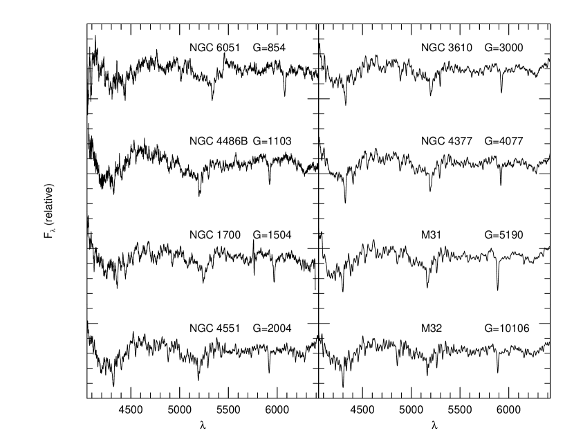
Figure 1: A selection of IDS spectra covering a range of S/N. Spectra are labelled with their name and goodness $G$ (see Section 3).

Briefly, spectra were obtained between 1972 and 1984 using the red-sensitive IDS and Cassegrain spectrograph on the 3m Shane Telescope at Lick Observatory. The spectra cover roughly 4000–6400 Å and have a resolution of about 9 Å (about 30% higher at the ends of the region) although this varied slightly from run to run. Most spectra of galaxy nuclei were taken through a spectrograph entrance aperture of $1\farcs 4$ by $4\arcsec$, with a second aperture for sky subtraction located $21\arcsec$ or $35\arcsec$ away. Object and sky were chopped between these apertures in such a way as to equalize the time spent in each. Long slit observations of galaxies (of width $1\farcs 4$ and various lengths) and spatial scans of globular clusters and galaxies were also taken and have equivalent resolution to the nuclear data. Larger-aperture observations of galaxies with wider slits (typically off-nucleus observations or dwarf galaxies) were also taken and calibrated separately. These wide-slit observations have lower spectral resolution. Helium, neon, mercury, and (in later observations) cadmium lamps provided wavelength calibrations at the beginning and end of every night. Global shifts and stretches of the wavelength scale of up to 3 Å per observation could occur due to instrument flexure and variable stray magnetic fields. Spectra were not fluxed, but rather divided by a quartz-iodide tungsten lamp, the energy distribution of which was made more constant with wavelength by “rocking” the dispersion grating in a reproducible, systematic manner. Line-strength standard stars (detailed in Paper V) were observed nightly to insure a calibration of the system. A sampling of low- to high-quality galaxy nuclei spectra are shown in Figure 1. For display purposes, these spectra have been flattened by a fifth-order polynomial fit. However, all measurements of line strengths were made on the original, unflattened spectra.

2.1 The Lick/IDS System

The Lick/IDS absorption-line index system is fully described in Paper V. We present a summary here and point out changes to the system caused by measuring galaxies with significant systemic velocities and velocity dispersions. Absorption-line strengths are measured in the Lick/IDS system by “indices,” where a central “feature” bandpass is flanked to the blue and red by “pseudocontinuum” bandpasses. The choice of bandpasses is dictated by three needs: proximity to the feature, less absorption in the continuum regions than in the central bandpass, and maximum insensitivity to velocity dispersion broadening. While the last point is unnecessary when measuring stars, in the case of galaxies it is crucial, and it sets a minimum length for the pseudocontinuum bandpasses. The sidebands are called “pseudocontinua” because the resolution of the Lick/IDS system does not allow the measurement of “true” continua in late-type stars or in most galaxies.

Table 2 presents the bandpasses of the 21 Lick/IDS absorption line indices and the features measured by these indices. The wavelengths have been further refined since Paper V through cross-correlation with more accurate CCD spectra taken by GW. Indices 1–8 have been corrected by $1.25$ Å, and indices 17–21 have been corrected by $1.75$ Å. Uncertainties of 0.3 Å are still present in these bandpass definitions, but such shifts produce negligible changes in the measured indices. Systemic velocities of the galaxies sometimes caused the reddest absorption features to fall outside of the wavelength range of the observation, and the starting wavelength of the spectra also varied somewhat. Occasionally other effects prevented the measurement of particular indices, including bubbles in the immersion oil of the IDS, exceptionally strong galaxy emission, or poorly-subtracted night sky lines (see Section 6 for a complete list). As a result, not all indices are measured for all galaxies.

The Lick/IDS index system was nominally designed to include six different molecular bands [CN4150, the G band (CH), MgH, MgH $+$ Mg $b$, and two TiO bands] plus 14 different blends of atomic absorption lines. The CN₂ index, introduced in Paper V, is a variant of the original CN₁ index with a shorter blue sideband to avoid H$\delta$. Along with the higher-order Balmer lines presented in Worthey & Ottaviani (1997), we believe we have extracted all of the useful absorption features from the Lick/IDS stellar and galaxy spectra.

We note here the recent work of Tripicco & Bell (1995), who modelled the Lick/IDS system using synthetic stellar spectra. They found that many of the Lick/IDS indices do not in fact measure the abundances of the elements for which they were named. Column 6 of Table 2 describes their results, in order of the most significant contributing element. To retain conformity with previously published studies we have chosen not to rename most of the Lick/IDS indices for their primary contributor. However, following Worthey, Trager & Faber (1996), we have renamed the Fe4668 index C₂4668.

2.2 Index measurements

Index measurements from the Lick/IDS galaxy spectra are problematic owing to unpredictable wavelength shifts and stretches (of order 1–3 Å) and also from the (sometimes unknown) systemic radial velocities of the galaxies themselves. Indices were measured automatically using the program AUTOINDEX written by J. J. González and G. Worthey. This program begins by locating Na D (centroid assumed at 5894 Å) and the G band (centroid assumed at 4306 Å) or, for a few galaxies with very strong Balmer lines, H$\gamma$ (centroid assumed at 4340 Å). It then removes any global wavelength shift and stretch, including the effects of the systemic velocity. Local wavelength shifts at each index are calculated by cross-correlating the galaxy spectrum with a template spectrum in the region around each index. For galaxies, a K0 giant template is generally used, but occasionally an F5 dwarf template is used for galaxies with very strong Balmer lines.

Once each index was centered, it is measured following the scheme outlined in Paper V. The mean height in each of the two pseudocontinuum regions is determined on either side of the feature bandpass, and a straight line was drawn through the midpoint of each one. The difference in flux between this line and the observed spectrum within the feature bandpass determines the index. For narrow features, the indices are expressed in Ångstroms of equivalent width; for broad molecular bands, in magnitudes. Specifically, the average pseudocontinuum flux level is

$$F_{P}=\int_{\lambda_{1}}^{\lambda_{2}}F_{\lambda}d\lambda/(\lambda_{2}-\lambda_{1}),$$ (1)

where $\lambda_{1}$ and $\lambda_{2}$ are the wavelength limits of the pseudocontinuum sideband. If $F_{C\lambda}$ represents the straight line connecting the midpoints of the blue and red pseudocontinuum levels, an equivalent width is then

$${\rm EW}=\int_{\lambda_{1}}^{\lambda_{2}}\left(1-{F_{I\lambda}\over F_{C\lambda}}\right)d\lambda,$$ (2)

where $F_{I\lambda}$ is the observed flux per unit wavelength and $\lambda_{1}$ and $\lambda_{2}$ are the wavelength limits of the feature passband. Similarly, an index measured in magnitudes is

$${\rm Mag}=-2.5\log\left[\left({1\over\lambda_{2}-\lambda_{1}}\right)\int_{\lambda_{1}}^{\lambda_{2}}{F_{I\lambda}\over F_{C\lambda}}d\lambda\right].$$ (3)

As explained in Paper V, the above AUTOINDEX definitions differ slightly from those used in Burstein et al. (1984) and Faber et al. (1985) for the original 11 IDS indices. In the original scheme, the continuum was taken to be a horizontal line over the feature bandpass, at the level $F_{C\lambda}$ taken at the midpoint of the bandpass. This flat rather than sloping continuum induces small, systematic shifts in the feature strengths, as described in further detail in Section 5. For now it is sufficient to note that slight additive corrections have been applied to the new indices to preserve agreement with the older published data. These corrections are discussed in Section 5 and are always quite small.

Run corrections for the galaxies also differ from those described for stars in Paper V. Stars always have nearly zero velocities, and their features occupy the same IDS channels on a given run. It was therefore found to be advantageous to apply small additive corrections to all indices to correct for small variations in continuum shape and/or resolution for that run. Galaxies however occupy different channels due their varying radial velocities, making the stellar-derived continuum shape corrections invalid. Hence, the following scheme was adopted, according to the velocity offset of a galaxy from the stars: globular clusters and galaxies with $cz\leq 300$ ${\rm km\ s^{-1}}$ (i.e., Local Group galaxies) had stellar run corrections applied for all indices; galaxies with $300<cz<10\,000$ ${\rm km\ s^{-1}}$ had stellar run corrections applied only to the broad molecular indices measured in magnitudes; and galaxies with $cz\geq 10\,000$ ${\rm km\ s^{-1}}$ had no run corrections applied.

3 Error Estimation

The errors of the IDS indices are due partly to photon statistics and partly to the fact that the flat-field calibration of the IDS had limited accuracy. A thorough knowledge of the errors is essential to the proper use of these data. The error estimates derived here will be used in later papers to simulate the absorption-line data and test the significance of any conclusions.

The IDS was not a true photon-counting detector. This makes estimation of uncertainties difficult, as the errors are not strictly photon counting statistics. We present in this section a brief overview of the steps required to derive reasonable error estimates for galaxy Lick/IDS index measurements. A complete discussion of the error estimates presented here may be found in Trager (1997).

In the IDS, light from the spectrograph fell on a series of three image-tube photocathodes, which amplified the signal by about $10^{5}$. The amplified light fell on a phosphor screen, which held the light long enough for an image dissector to scan and digitize the image before it faded (Robinson & Wampler (1972)). Each incident photon produced a burst of typically seven to ten detected photons covering $\sim 9$ Å (7 channels) in the digitized scan. Uncertainties in the spectra arise from three sources: (1) input photon shot noise, (2) the statistics of the amplification process, and (3) flat-fielding errors. This last noise source is due to the movement of the spectrum of the first photocathode, caused by instrument flexure, and movement of the amplified spectrum, caused by stray magnetic fields affecting the magnetically-focused image-tubes and image dissector. As a result, flat-field spectra taken at different telescope locations and position angles do not divide perfectly but rather show low-level undulations a few channels wide.

The effect of these three noise sources on the power spectrum is discussed in Dalle Ore et al. (1991), Paper V, and Trager (1997). At low frequencies the noise is dominated by flat-fielding errors (at high counts) and photon shot-noise and the statistics of the IDS burst amplification process (at low counts). At high frequencies the noise is dominated by flat-fielding errors (very high counts) and photon statistics (low and moderate counts). The resultant power spectrum changes shape with count level, as shown schematically by Trager (1997). In galaxy spectra, photon statistics tend to be the overall dominant noise source, as opposed to the stellar spectra (Paper V) and the highest-signal-to-noise galaxies (e.g., M31 and M32), in which flat-fielding errors dominate.

The net result is that the high-frequency noise is a good measure of photon statistics except at very high count levels, where flat-fielding errors begin to dominate. Paper V therefore defined a “goodness parameter” that measures the noise power at high frequencies. For each spectrum, a Fourier transform was taken of the 256 channels starting at 5519 Å in the rest frame, a region relatively free of spectral lines. The average power at high spatial frequencies was measured, then divided by the power at zero frequency. The square root of this ratio is a measure of photon noise, and its inverse is defined to be the goodness $G$.

$G$ is defined such that, if all noise were photon statistics, $G$ would be exactly proportional to $\sigma^{-1}$. The constant of proportionality is unknown a priori (it depends on the average number of detected photons per burst, which is not well known) but can be determined empirically by comparing to errors derived from multiply-observed data. At high count levels, $G$ saturates (bottoms out) due to the influence of flat-field errors, and the relation of $G$ to $\sigma^{-1}$ becomes non-linear. This curvature can also be determined empirically from multiply-observed objects.

The empirical calibration proceeds as follows. Because $G$ scales as $\sigma^{-1}$ for poor data, it should average quadratically for multiple observations, and thus we compute the goodness $\langle G\rangle_{k}$ of a single, typical observation of galaxy $k$ as

$$\langle G\rangle_{k}^{2}={1\over N}\sum G_{i,k}^{2},$$ (4)

where $G_{i,k}$ is the goodness of each individual spectrum and $N$ is the number of observations of galaxy $k$. $\langle G\rangle_{k}$ would be the goodness of each single observation of galaxy $k$ if all observations were of equal quality. All galaxies with three or more observations had average goodnesses computed by Equation 4. The same galaxies also had mean standard deviations computed for each of the 16 Lick/IDS indices between the G band and Na D (in the spectral range of virtually all galaxies). The average total error $\sigma_{{\rm TOT},k}$ of galaxy $k$ averaged over these 16 indices is calculated as

$$\sigma^{2}_{{\rm TOT},k}={1\over 16}\sum^{19}_{j=4}\left({\sigma_{jk}\over\sigma_{sj}}\right)^{2},$$ (5)

where $j$ is the IDS index number (Table 2), $\sigma_{jk}$ is the standard deviation per observation of index $j$ for galaxy $k$, and $\sigma_{sj}$ is the standard star error of index $j$ (Table 2). Thus $\sigma_{{\rm TOT},k}$ is the average error in units of the standard star error for a typical single observation of galaxy $k$. It is an external error determined from multiple, independent observations of the same object.

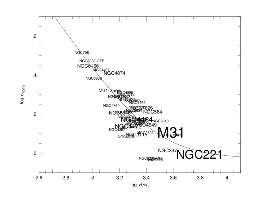
Figure 2: Preliminary calibration of the independently determined error $\sigma_{{\rm TOT},k}$ with goodness $\langle G\rangle_{k}$. The size of the galaxy labels is proportional to the number of observations. The middle of the label is the location of the point. The relation flattens at high $\langle G\rangle_{k}$ due to flat-fielding errors. The solid line is a least-squares linear fit to the relation $\sigma^{2}_{{\rm TOT},k}=a\langle G\rangle_{k}^{-2}+b$ (see Section 3).

To determine a preliminary scaling of total error with goodness, individual total errors $\sigma_{{\rm TOT},k}$ were plotted against average goodnesses $\langle G\rangle_{k}$ (Figure 2). There is a reasonably tight relation between the two with the expected trend. The slope is $-1$ in the low-signal limit, where photon statistics dominate, and flattens out in the high-signal limit, where flat-fielding errors dominate. The solid curve is a least squares fit to the equation $\sigma^{2}_{{\rm TOT},k}=a\langle G\rangle_{k}^{-2}+b$:

$$\sigma^{2}_{{\rm TOT},k}=\left({2561\over\langle G\rangle_{k}}\right)^{2}+(0.94)^{2}.$$ (6)

Equation 6 is assumed to hold for each individual observation, with $\langle G\rangle_{k}$ replaced by $G_{i,k}$. Weighted mean indices for multiply-observed galaxy $k$ are calculated as

$$\langle I_{jk}\rangle=\left(\sum_{i=1}^{N}I_{ijk}/\sigma^{2}_{{\rm TOT},i,k}\Bigl{/}\sum_{i=1}^{N}1/\sigma^{2}_{{\rm TOT},i,k}\right),$$ (7)

where $i$ represents an individual observation, $j$ represents a given index, and $\sigma_{{\rm TOT},i,k}$ is now derived from $G_{i,k}$ using Equation 6.

Finally, the error of each mean index $j$ is taken to be

$$\sigma_{jk}=\frac{1}{\sqrt{N}}\sigma_{{\rm TOT},k}\times\sigma_{sj},$$ (8)

where $N$ is the number of observations of galaxy $k$, $\sigma_{sj}$ is the standard star error, and the mean error of galaxy $k$ for all indices, $\sigma_{{\rm TOT},k}$, is calculated from Equation 6, using $\langle G\rangle_{k}$ determined as in Equation 4. This version of $\sigma_{jk}$ is more accurate than the individual index standard deviations because it uses the average error per spectrum, $\sigma_{{\rm TOT},k}$, made possible by knowing the ratios of the errors between indices from the standard stars.

We then set out to check the quality of these preliminary error estimates. We were interested in both the magnitude of the errors averaged over all indices and the ratio of the individual index errors. To anticipate the results, we found that the mean magnitude of the galaxy errors was well determined (to within 8%) but that certain individual error ratios needed adjustment.

The details of this step are given in Trager (1997) but a brief description follows. Independent nuclear data from galaxies in the sample of González (1993; hereafter G93) were compared against individual observations of 37 IDS galaxies in common. The G93 spectra cover only the region 4780–5600 Å, and so only the indices from H$\beta$ through Fe5406 could be compared. A chi-squared analysis was performed to determine the relative scaling of the Lick/IDS galaxy errors with respect to G93. González’s indices are so accurate (except for Mg₁ and Mg₂) that his errors contribute negligibly, and the resultant $\chi^{2}$ values are a good test of the Lick/IDS errors alone. Though we expect the errors in G93 to be negligible, we allowed for mean zeropoint and slope differences, as González could not calibrate his CCD system precisely onto the IDS system (see his Figure 4.4). The error rescalings determined from the G93 comparison were fairly small, about $0.92$. The exception was Fe5270, which required a large error rescaling (0.75; i.e., the preliminary IDS errors from Equation 8 above were too large by 25% in this index).

A further check for wavelengths not covered by the G93 spectra was performed using pairs of indices from the Lick/IDS sample itself. Indices were chosen that might be expected a priori to track each other closely (i.e., to be multiples of one another) and have similar velocity dispersion corrections. The best choices came from the Fe-peak family of indices (see Section 4.4, although note that these indices do not all track Fe abundance—see Tripicco & Bell 1995 and Table 2). Two groups were defined by their similar velocity dispersion corrections: Fe4383, Fe4531, and Fe5709 were compared against Fe5270; and Fe5782 and Ca4455 were compared against Fe5335. The errors of Fe5270 and Fe5335 were first rescaled to match G93 as described above. Chi-squared analyses were performed, and the resultant reduced-$\chi^{2}$ value was forced to equal unity by rescaling the Lick/IDS errors of the dependent index. The error rescalings from these internal comparisons are comparable to those derived from the G93 comparison, typically again about $0.92$.

A final mean fractional error scaling was then computed from all scalings derived in these tests. This mean scaling was again $0.92$. Errors in the remaining 10 indices were rescaled by this factor. We checked the final adopted index scalings by performing a final set of chi-squared tests on various Fe-line pairs. The resulting reduced-$\chi^{2}$ values were consistent with our final scaling of the errors to typically within a few percent (and never worse than 5%). From these various tests, we believe that systematic errors in the final uncertainties are $\lesssim 5\%$.

The adjusted final errors for the raw indices of all galaxies and globular clusters are computed as

$$\sigma_{j}^{adj}=c_{j}\sigma_{j},$$ (9)

where $\sigma_{j}$ is the preliminary error of index $j$ computed in Equation 8, and $c_{j}$ is the scaling of index $j$ relative to the standard star indices as determined in these tests. Adopted values of $c_{j}$ are shown in Table 3.

4 Velocity Dispersion Corrections

The observed spectrum of a galaxy is the convolution of the integrated spectrum of its stellar population by the instrumental broadening and the distribution of line-of-sight velocities of the stars. The instrumental and velocity-dispersion broadenings broaden the spectral features, causing the absorption-line indices to appear weaker than they intrinsically are. In this section, we discuss the corrections required to remove the effects of velocity dispersion from the galaxy index measurements and the additional uncertainties that arise from these corrections.

4.1 Velocity dispersion data

The adopted nuclear galaxy velocity dispersions, their fractional errors, and their sources are presented in Table 4. The majority of the velocity dispersions was derived directly from the IDS spectra themselves. The basic method was discussed in Dalle Ore et al. (1991), and the data were presented in Davies et al. (1987, as tabulated by Faber et al. 1989) and Dalle Ore et al. Other sources of nuclear dispersions include G93, the compilation of Faber et al. (1997), and the compilation of Whitmore, McElroy & Tonry (1985), in order of preference. The velocity dispersions of both Whitmore et al. and Faber et al. are derived from comprehensive literature searches, but the data of G93 are excellent and uniform (and supersede all other measurements when available). Two other sources noted in Table 4 (Bender, Paquet & Nieto 1991; Peterson & Caldwell 1993) were used for dwarf galaxies. For a few galaxies, no velocity dispersions were available, so educated guesses were made by eye or by comparing against similar galaxies with known velocity dispersions These rough velocity dispersions are derived for the purpose of velocity dispersion corrections only and should not be used for any other purpose. They are indicated in Table 4 as Source 8.

For off-nuclear observations of galaxies (Table Old Stellar Populations. VI. Absorption-Line Spectra of Galaxy Nuclei and Globular Clusters), velocity dispersions were calculated as

$$\sigma_{r}=\sigma_{0}\left({r\over 1\farcs 4}\right)^{-0.06},$$ (10)

where $r$ is the radius at which the aperture was placed and $\sigma_{0}$ is the velocity dispersion given in Table 4. The exponent is a mean for early-type galaxies as determined from Figure 6.10 of G93.

Finally, a few galaxy nuclei were observed by scanning a long slit of dimensions $1\farcs 4\times 16\arcsec$ across the nucleus to create a $16\arcsec\times 16\arcsec$ aperture (denoted “scan” in Table Old Stellar Populations. VI. Absorption-Line Spectra of Galaxy Nuclei and Globular Clusters). These were observed to determine aperture corrections to velocity dispersion and Mg₂ in Davies et al. (1987). For these we have used the velocity dispersions as corrected by Equation 1 of Davies et al.

4.2 Corrections from broadened stellar spectra

To correct absorption-line strengths for the effects of velocity dispersion, a reference velocity dispersion must be chosen. As we plan to compare the indices derived in this study to stellar-population models based on our stellar observations (Paper V, Worthey 1994), the indices are corrected to zero velocity dispersion. To achieve this goal, a variety of stellar spectra was convolved with broadening functions of various widths. A selection of G dwarfs and the K giant standard stars was convolved with Gaussians of widths ranging up to $\sigma=450$ ${\rm km\ s^{-1}}$. Index strengths were measured from each convolved spectrum and compared to the original strengths. A third-order polynomial was then fit to the ratios (original/convolved) for all the stars in each index versus velocity dispersion. Several observations of M32 were also included in the fits (M32 has a very small velocity dispersion compared to the resolution of the IDS system). Figure 3 shows the results of these fits, and Table 5 presents the coefficients of the polynomials.

A velocity-dispersion corrected index is then

$$I_{j,k}^{corr}=C_{j}(\sigma_{v})\times\langle I_{j}\rangle_{k},$$ (11)

where $\langle I_{j}\rangle_{k}$ is the mean value of index $j$ of galaxy $k$ from Equation 7, and $C_{j}(\sigma_{v})$ is the velocity-dispersion correction:

$$C_{j}(\sigma_{v})=\sum_{i=0}^{3}c_{ij}\sigma_{v}^{i},$$ (12)

where $c_{ij}$ are the coefficients of the correction polynomial for index $j$ (Table 5), and $\sigma_{v}$ is the velocity dispersion.

Figure 3 shows that considerable scatter exists in certain velocity-dispersion corrections. As noted by G93, a variation with spectral type is seen in several indices. Some of the scatter is negligible, reflecting variations in indices that are intrinsically small (Mg₁, TiO₁, TiO₂). Scatter in CN₁, CN₂, and H$\beta$ is real. However, CN is not heavily used, while the scatter in H$\beta$ is inflated due to the inclusion of a few very cool K giants with H$\beta$ strengths weaker than typical galaxies. In what follows, we do not assign any uncertainty to the velocity dispersion corrections. The uncertainty in the H$\beta$ correction will be noted in future papers when applicable.

4.3 Final errors

The velocity-dispersion corrections increase the raw index errors, $\sigma_{j}$, by the value of the multiplicative correction. An additional source of uncertainty is introduced by errors in the velocity dispersion estimates themselves. It proves simplest to discuss these effects in terms of the fractional error of the final index.

The uncertainty from the velocity dispersion error is computed as the fractional uncertainty of the galaxy’s velocity dispersion multiplied by the derivative of the correction function at that velocity dispersion:

$$\sigma_{v,j}=\epsilon_{\sigma_{v}}{d\ln C_{j}\over d\ln\sigma_{v}},$$ (13)

where $\sigma_{v,j}$ is the fractional uncertainty in the velocity-dispersion correction of index $j$, $\epsilon_{\sigma_{v}}$ is the fractional uncertainty of the velocity dispersion estimate, $C_{j}$ is the velocity-dispersion correction of index $j$ (Equation 12), and $\sigma_{v}$ is the velocity dispersion. This uncertainty is added in quadrature with the raw fractional error in the index $j$,

$$\sigma_{f,j}^{2}=\sigma_{v,j}^{2}+\left({\sigma_{j}^{adj}\over\langle I_{j}\rangle}\right)^{2},$$ (14)

where $\sigma_{f,j}$ is the final fractional uncertainty of index $j$, $\sigma_{j}^{adj}$ is the raw error of index $j$ (Equation 9), and $\langle I_{j}\rangle$ is the value of index $j$ uncorrected for velocity dispersion. The final fractional error is then multiplied by the velocity-dispersion corrected index $j$, $I_{j}^{corr}$ (Equation 11), to determine the final, corrected error of index $j$:

$$\sigma_{j}^{corr}=\sigma_{f,j}\times I_{j}^{corr}.$$ (15)

4.4 Index families

Figure 5 presents the indices as a function of Mg₂ before (Figure 5a) and after (Figure 5b) velocity-dispersion correction for all galaxy observations through the nominal aperture ($1\farcs 4\times 4\arcsec$; Figures 5 and 7 include nuclear and non-nuclear observations). Almost all line-strength–Mg₂ distributions tighten slightly, except H$\beta$–Mg₂, in which the scatter increases somewhat since the velocity dispersion corrections multiply the scatter already present. Figure 7 presents the indices as a function of velocity dispersion after velocity-dispersion correction for the same galaxies. In Figure 5, a tail of points to lower index values is visible for strong-lined objects in both H$\beta$ and Fe5015. This tail is due to residual emission-line contamination in a few objects.

After correction, indices seem to fall into three general families: (1) $\alpha$-element-like indices, including both CN indices, all three Mg indices, Na D, and TiO₂, characterized by relatively narrow, positive correlations with both Mg₂ and velocity dispersion; (2) Fe-like indices, including both Ca indices, the G band, TiO₁, and all Fe indices, with quite broad distributions that are only weakly correlated with Mg₂ and velocity dispersion; and (3) H$\beta$, which acts inversely to the $\alpha$-element indices, with a relatively narrow, negative correlation with Mg₂ and velocity dispersion. Similar correlations were seen in a restricted set of indices by Burstein et al. (1984), Carollo et al. (1993) and Jørgensen (1997). C₂4668 seems to be intermediate to the $\alpha$- and Fe-like indices, with a relatively broad, but positive correlation with Mg₂ and velocity dispersion. These groupings probably represent element abundance families with different nucleosynthesis histories, as discussed in Worthey (1996).

5 Remaining Systematic Errors

We now estimate the remaining systematic errors in the Lick/IDS data. Even small systematic errors are a source of concern because indices change only slightly over time for old stellar populations, so that small index differences can translate to significant age differences. For example, a systematic error in the key H$\beta$ index of only 0.05 Å corresponds to a model age difference of $\sim$ 1 Gyr at 15 Gyr (Worthey 1994).

There are two potential sources of inhomogeneities, and thus systematic errors, in the data. One comes from the use of two measurement schemes, the original scheme described by Burstein et al. (1984) (hereafter called “eye”) and the current scheme used here and for many stars in Paper V (called “AUTOINDEX”). The second source of error comes from the presence of two separate instrumental systems (for the first 11 indices only) — an earlier one (called “old”) based on standardizing to mean data for K giant standards in Runs 3–24, and a second one (called “new”) based on K giant standards from all runs. The original 11 indices published for K giants (Faber et al. 1985) and G dwarfs (Gorgas et al. 1993) were measured with the eye method and transformed to the old system, whereas the new stellar data in Paper V and the galaxy and globular data measured here were measured with AUTOINDEX and transformed (at least initially, see below) to the new system. We therefore consider (1) systematic differences in raw measurements between the eye and AUTOINDEX schemes and (2) any zeropoint differences and their uncertainty between the old and new standard systems. We stress that these issues exist only for the 11 original indices; the 10 new indices added in Paper V have always been measured using AUTOINDEX and standardized to the K giant data from all runs.

5.1 Measurement systematics

We begin with a comparison of the eye and AUTOINDEX schemes; there are two principal differences between them.

1. Centering of feature bandpasses. In the eye scheme, wavelength errors were corrected by centering feature bandpasses by eye using a reference stellar spectrum. AUTOINDEX centers features automatically by performing a cross-correlation of the object spectrum with a template stellar spectrum. These automatic centerings were then checked visually by eye.

2. Continuum determination. As discussed in Section 2.2, the eye scheme took the continuum to be horizontal over the feature bandpass at a level $F_{C\lambda}$ measured at the midpoint of the bandpass. In the AUTOINDEX scheme, the continuum slopes over the feature bandpass. The difference in continuum shapes potentially induces small, systematic shifts in the feature strengths.

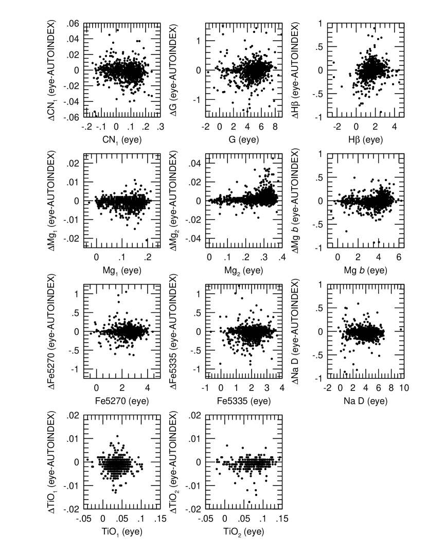
Figure 10: IDS measurement scheme differences, eye$-$AUTOINDEX, for all galaxy and globular cluster observations (including off-nuclear and wide-slit observations), as a function of eye measurements. Run and velocity-dispersion corrections have not been applied.

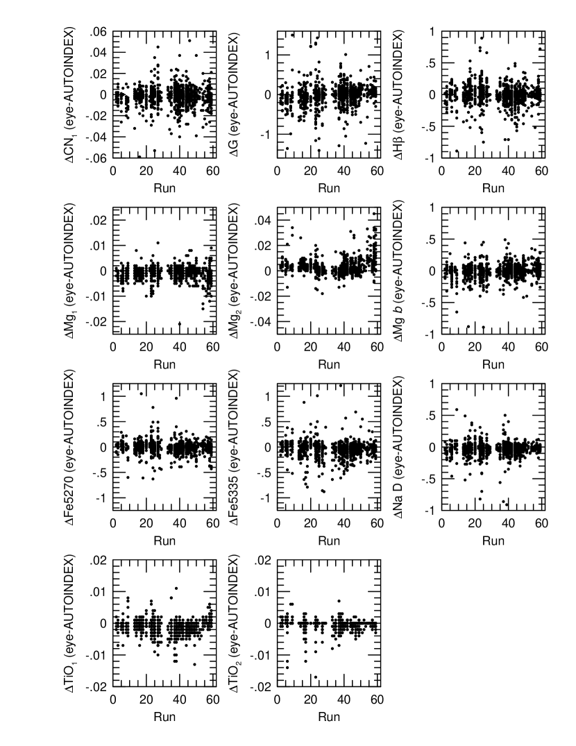
Figure 11: IDS measurement scheme differences, eye$-$AUTOINDEX, for all galaxy and globular cluster observations (including off-nuclear and wide-slit observations), as a function of IDS run number. Run corrections have not been applied.

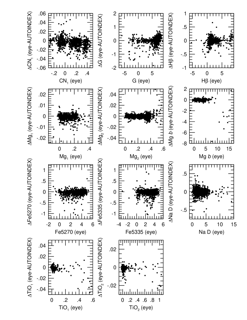
Figure 12: IDS measurement scheme differences, eye$-$AUTOINDEX, for all stars in Paper V, as a function of eye measurements. Run corrections have not been applied.

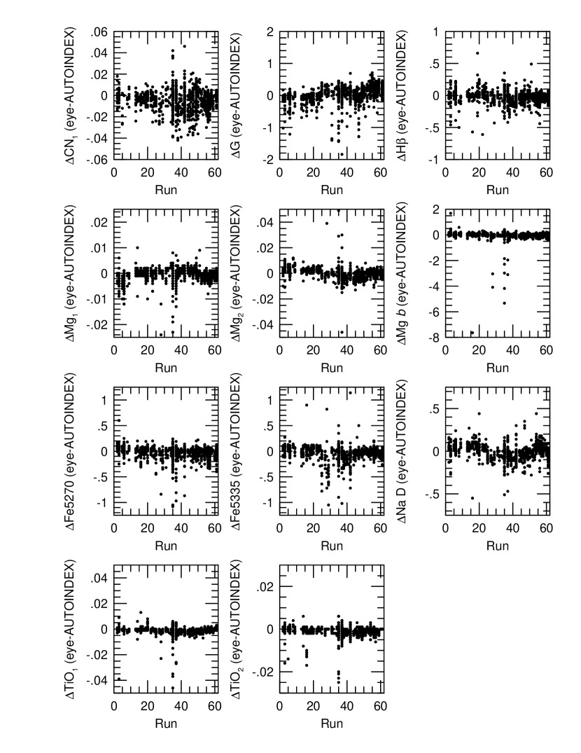
Figure 13: IDS measurement scheme differences, eye$-$AUTOINDEX, for all stars in Paper V, as a function of IDS run number. Run corrections have not been applied.

Figures 10–13 investigate these potential errors by plotting the quantity (eye$-$AUTOINDEX) for stars and galaxies (including globular clusters) separately. All galaxy and globular cluster observations are plotted in Figures 10 and 11, including off-nucleus and non-standard aperture size observations (i.e., all observations represented in Tables Old Stellar Populations. VI. Absorption-Line Spectra of Galaxy Nuclei and Globular Clusters–Old Stellar Populations. VI. Absorption-Line Spectra of Galaxy Nuclei and Globular Clusters are including in these Figures). All of these are raw values with no run or velocity dispersion corrections applied.

Figures 10 and 12 plot (eye$-$AUTOINDEX) vs. eye values. Most of the outlying points are either M stars (Fig. 12) or very noisy galaxy spectra (Fig. 10). For either, small centering differences between the two schemes can make large differences in the index values. A few residual distributions are also skewed toward negative values (e.g., Fe 5270, Fe5335). This probably results from the systematically better index centering in AUTOINDEX, which results in larger index values. However, these effects are small.

Figures 11 and 13 plot (eye$-$AUTOINDEX) vs. run number. Run-to-run differences are seen of order $\leq 0.2$ Å and $\leq 0.010$ mag, reflecting changes in instrumental response (i.e., spectral shape) among runs. (These are about half the size of the applied run corrections). However, large-scale, systematic trends that affect a large fraction of the data are at most half this size.

Of concern from the standpoint of systematic errors is any global shift or tilt between the two measuring schemes. Mean differences between eye and AUTOINDEX are summarized in Table 6 for stars and galaxies separately. Except for CN₁, global shifts are generally very small, $\leq 0.04$ Å and $\leq 0.003$ mag. CN₁ shows an offset of 0.005 mag for stars, plus a tilt of comparable size (see Fig. 12). Both effects were mentioned in Paper V, but neither seems to be present for galaxies and globular clusters (cf. Fig. 10). Neither the origin of these trends nor the difference between stars and galaxies are understood.

Summarizing the information in Figures 10–13 and Table 6, we conclude that large-scale, systematic differences between the eye and AUTOINDEX measuring schemes are generally $\leq 0.05$ Å and $\leq 0.003$ mag, with the exception of CN₁, for which the differences are twice as large.

We turn now to differences between the “old” and “new” standard systems. Recall that the standard system for the 11 original indices (here called the “old” system) was standardized to the K giant standards in Runs 3 – 24, about one-third of the data. In hindsight, we see that these early runs were atypical in some indices and that the standard system is therefore slightly “off” with respect to the whole data. Rather than change zeropoints now, since many data have been published and fitting-functions derived from them (Gorgas et al. 1993; Paper V), we compute zeropoint corrections needed to transform AUTOINDEX plus its new system of run corrections to the old, published system. The adopted corrections, based on the 9 K giant standard stars, are given in the last column of Table 6; they are applied to all the galaxy and globular data in this paper. For most indices, the corrections are quite small, a few hundredths of an Å or a few thousandths of a magnitude. The significant exception is the G-band, for which the offset is 0.21 Å. A previous, similar analysis in Paper V yielded the corrections shown in the second-to-last column. These shifts were used to correct the new stellar data in Paper V. The differences between the two sets of corrections are again at most a few hundredths of an Å or a few thousandths of a magnitude. These are small to negligible in the context of old stellar-populations. The differences between the Paper V and present corrections are a measure of the irreducible zeropoint uncertainties inherent in the published Lick/IDS system.

5.2 Mg₂: Comparison with Seven Samurai

Finally, we examine the Mg₂ values presented here with respect to those of the Seven Samurai (Davies et al. (1987), Faber et al. (1989)). Davies et al. (1987) used a combined Mg₂ index that weighted contributions from Mg₂ and Mg₁, both measured using the eye scheme. The resulting Mg₂ index is hereafter called $\langle\rm Mg_{2}\rangle$ to distinguish it from the Lick/IDS index Mg₂. We reproduce Equations 2 and 3 of Davies et al. here:

$$\rm Mg_{2}^{\prime}=0.03+2.10\,Mg_{1}-62\,Mg_{1}^{4},$$ (16)

$$\rm\langle{Mg_{2}}\rangle=0.6\,Mg_{2}+0.4\,Mg_{2}^{\prime}.$$ (17)

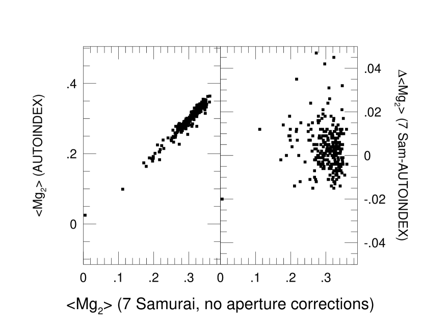
Figure 14: Comparison of IDS and Seven Samurai measurements of $\langle\rm Mg_{2}\rangle$. Data for Seven Samurai measurements are taken from Davies et al. (1987), without aperture corrections to Coma.

We have recomputed $\langle\rm Mg_{2}\rangle$ using the AUTOINDEX measurements for all galaxies in common between the two samples (Seven Samurai and that presented here). After removing the aperture correction to the Seven Samurai measurements (Equation 4 of Davies et al.), we compare the results in Figure 14. The mean difference (Seven Samurai$-$AUTOINDEX) is $+0.003$ mag, with a standard deviation of 0.010. This difference is close to what one would expect from comparing of the eye and AUTOINDEX schemes for Mg₂ in Table 6. The dispersion is also expected from a close examination of Figure 10. We recommend that those interested in using $\langle\rm Mg_{2}\rangle$ for Lick galaxies recompute this index from the values of Mg₁ and Mg₂ given here.

6 Final Absorption-Line Indices

Table Old Stellar Populations. VI. Absorption-Line Spectra of Galaxy Nuclei and Globular Clusters presents final mean velocity-dispersion-corrected indices, rms errors and total goodnesses $\sqrt{N_{obs}}\langle G\rangle$ for all galaxy nuclei observed through the nominal slit width and length ($1\farcs 4\times 4\arcsec$).

Table Old Stellar Populations. VI. Absorption-Line Spectra of Galaxy Nuclei and Globular Clusters presents similar data for nearly all globular clusters in the sample. Globular clusters have stellar run corrections applied to all indices. The values in Tables Old Stellar Populations. VI. Absorption-Line Spectra of Galaxy Nuclei and Globular Clusters and Old Stellar Populations. VI. Absorption-Line Spectra of Galaxy Nuclei and Globular Clusters supersede all previously published Lick/IDS galaxy and globular cluster index strengths. Galactic globular clusters were scanned over the cluster through a $1\farcs 4\times 16\arcsec$ slit to synthesize a 66″$\times$66″ aperture (cf. Burstein et al. 1984). Entries marked “O” are off-center observations through a similarly scanned aperture displaced 35″ away from the main aperture.

Table Old Stellar Populations. VI. Absorption-Line Spectra of Galaxy Nuclei and Globular Clusters presents data for galaxies observed through the nominal aperture of $1\farcs 4\times 4\arcsec$ but off the nucleus. The offset from the nucleus in arcseconds is marked next to the galaxy name. See the notes for details.

Table Old Stellar Populations. VI. Absorption-Line Spectra of Galaxy Nuclei and Globular Clusters presents data for observations through non-standard apertures. These were mostly off-nuclear measurements of bright galaxies, plus a few wide-slit nuclear observations of small galaxies and two globular clusters (the M31 globulars V29 and V92). The slit was widened to increase signal-to-noise. The offset from the nucleus (typically in arcseconds) is marked next to the galaxy name, if applicable. See the notes for details. Column 2 lists the aperture dimensions; entries marked “scan” in Column 2 were spatially scanned over a $16\arcsec\times 16\arcsec$ area through a $1\farcs 4\times 16\arcsec$ slit. Standard run corrections were applied as described in Section 2.2. K giant standard stars observed through wide slits were confirmed to have run corrections consistent with those observed through the nominal slitwidth.

In order to bring the wide-slit galaxy observations in Table Old Stellar Populations. VI. Absorption-Line Spectra of Galaxy Nuclei and Globular Clusters onto the Lick/IDS system, a correction for slitwidth broadening was made that was similar to the velocity dispersion correction. Figure 8 shows a plot of the K giant standard star indices measured through wide slits as a function of slit width (compare to Figure 3). Observations through $1\farcs 8$- and $2\farcs 2$- slits were judged usable without need for correction. For observations through the $3\farcs 4$-, $5\farcs 4$-, and $7\farcs 4$-wide slits, the median values of the K giant ratios of mean index strength through the nominal slit to the wide-slit index strengths were used to correct the index values and raw errors. These multiplicative corrections are listed in Table 11. The strengths of Ca4227, Ca4455, Fe4531, H$\beta$, Fe5015, Fe5335, Fe5406, Fe5709, and Fe5782 were all judged to be unusable for observations through the $7\farcs 4$-wide slit due to the large dispersion in the K giant ratios of Figure 8. These indices are not listed for this aperture in Table Old Stellar Populations. VI. Absorption-Line Spectra of Galaxy Nuclei and Globular Clusters.

Some index measurements are missing from Tables Old Stellar Populations. VI. Absorption-Line Spectra of Galaxy Nuclei and Globular Clusters–Old Stellar Populations. VI. Absorption-Line Spectra of Galaxy Nuclei and Globular Clusters. There are five possible reasons: (1) The spectral coverage of the IDS system was not consistent throughout all runs, and the CN indices or TiO indices may not have been observed (this is more likely for galaxies observed only once). (2) Ephemeral features caused by bubbles in the immersion oil of the photomultiplier chain may have contaminated certain index measurements. (3) The systemic velocity of the galaxy may have moved the reddest indices (TiO₁ and TiO₂) out of the spectral range of the IDS system. (4) Intrinsic emission such as H$\beta$ or [O 3] $\lambda 5007$ in the galaxy may have contaminated a central bandpass or sideband. We have culled the most obvious examples of emission contamination, but subtle contamination remains. Users of these data should be aware of this. (5) Poorly-subtracted night-sky lines contaminated certain indices. Table 12 presents a list of indices possibly affected by residual contamination from poor night-sky subtraction.

7 Summary

This paper presents the complete database of Lick/IDS absorption-line index strengths for galaxies and globular clusters. This database supersedes all previously published Lick/IDS data on these objects. The Lick/IDS galaxy data are among the largest collection of homogeneous absorption-line strengths for stars and galaxies currently available.

We have reviewed the measurement of Lick/IDS indices from IDS spectra and characterized the errors. The level of remaining systematic uncertainties is discussed. We also present for the first time the correction of Lick/IDS absorption-line strengths for velocity dispersion. Such a correction is a crucial step to compare Lick/IDS galaxy absorption-line strengths to models of stellar populations based on the Lick/IDS stellar library (Worthey (1994)).

In a subsequent paper, we will present an analysis of a subset of these data using stellar population models in an attempt to derive stellar population ages, metallicities, and relative element abundances of the nuclei of early-type galaxies.

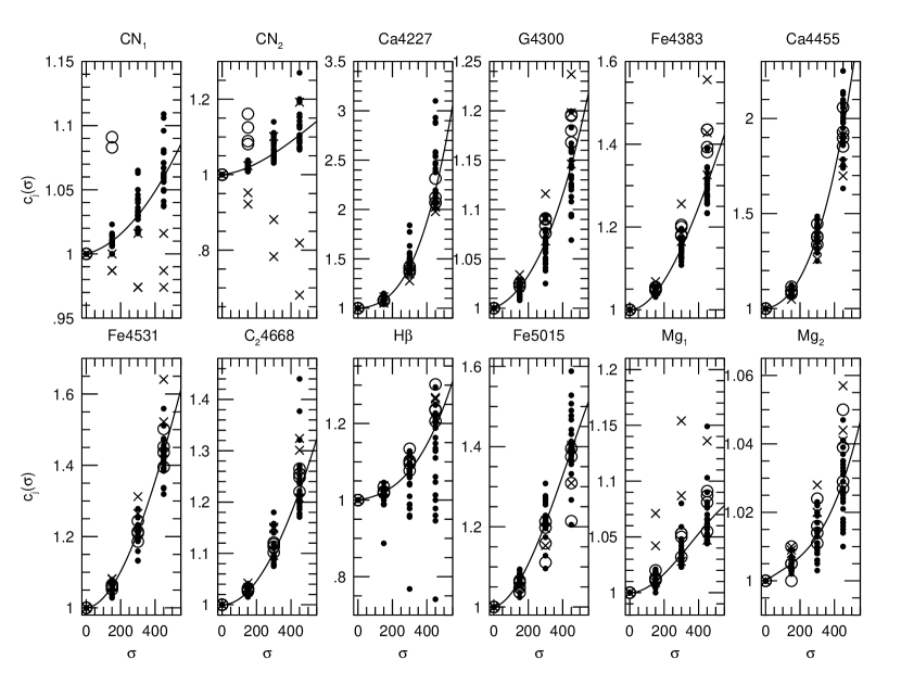
Figure 3: Multiplicative index correction, $C_{j}$, as a function of velocity dispersion (in ${\rm km\ s^{-1}}$) for all 21 Lick/IDS indices. The corrections have been determined by measuring various stellar spectra convolved to different broadenings. Symbols represent K giant standard stars (small dots), G dwarfs (crosses), and M32 (multiple observations; open circles). The quantity shown is index(0)/index($\sigma$).

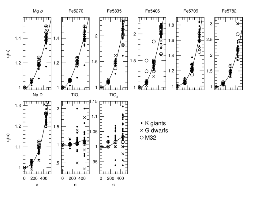
Figure 3: Continued.

Figure 5: Index strengths as a function of Mg₂ (in mag) for all 21 Lick/IDS indices for all galaxy observations (nuclear and off-nuclear) through the standard $1\farcs 4\times 4\arcsec$ aperture. (a) Before velocity-dispersion correction.

Figure 4: (b) After velocity-dispersion correction.

Figure 7: Index strengths as a function of velocity dispersion (in ${\rm km\ s^{-1}}$) for 20 Lick/IDS indices (all except CN₂, which reproduces the behavior of CN₁ very closely) for all galaxy observations (nuclear and off-nuclear) through the standard $1\farcs 4\times 4\arcsec$ aperture, after velocity-dispersion correction.

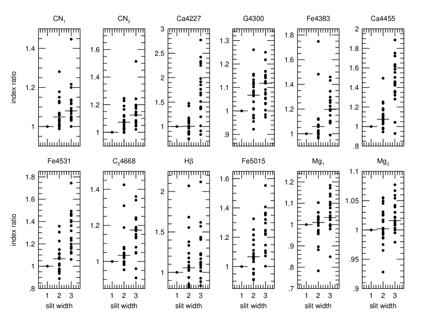
Figure 8: Multiplicative index corrections as a function of slitwidth (1=nominal slitwidth, $1\farcs 4$; 2=$3\farcs 4$; 3=$7\farcs 4$) for all 21 Lick/IDS indices, for K giant standard stars. The vertical axis is index($1\farcs 4$)/index(slitwidth). Horizontal lines are the corrections applied at each slitwidth. Missing horizontal lines denote indices deemed too uncertain at $7\farcs 4$ to be useful.

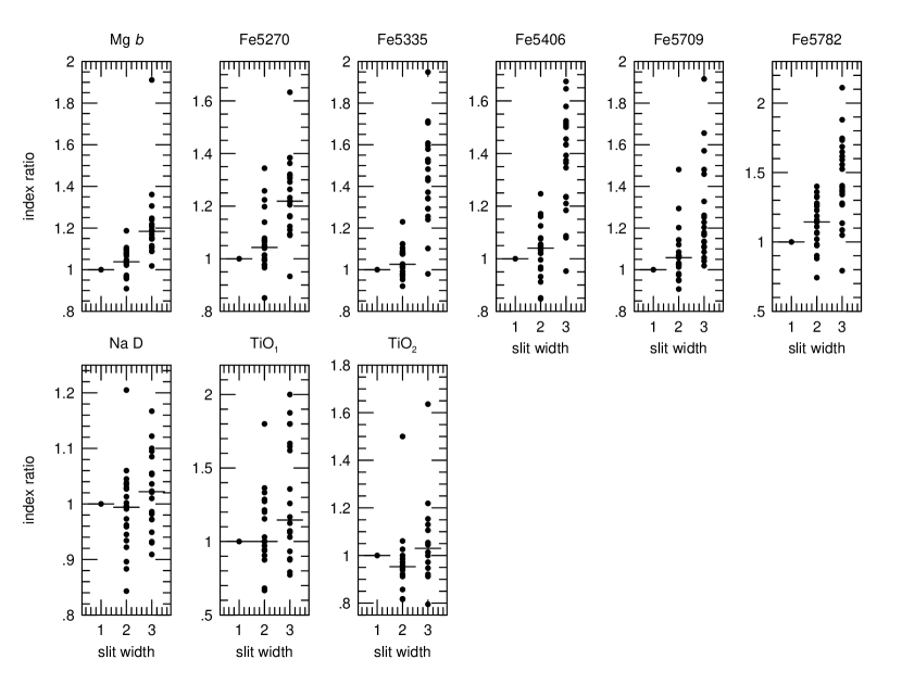
Figure 6: Continued.

Table 1: Published IDS Data

Paper	No. of Indices	Method	Run corrections
(a) Galaxies and Globular Clusters
Burstein et al. (1984) globulars	11	E	all indices
Davies et al. (1987)	$\langle{\rm Mg_{2}}\rangle$	E	yes
Burstein et al. (1988)	$\langle{\rm Mg_{2}}\rangle$	E	yes
Worthey, Faber, & González (1992)	Mg2, Fe5270, Fe5335	A	Mg2 only
This paper
Galaxies	21	A	molecular bands only
Globulars, low-velocity galaxies	21	A	all indices
(b) Stars
Faber et al. (1985) K giants	11	E	all indices
Burstein et al. (1986)	Fe5270, Fe5335	E	all indices
Gorgas et al. (1993) G dwarfs	11	E	all indices
Worthey et al. (1994)
Prev. published K giants, G dwarfs	11	E	all indices
	+10	A	all indices
All other stars	21	A	all indices

Note. — Columns:

(1) Reference

(2) Number of indices published: 11=original 11 Lick/IDS indices of Burstein et al. (1984); 21=all Lick/IDS indices (see Table 2); +10=new indices presented in Worthey et al. (1994); $\langle{\rm Mg_{2}}\rangle$=“average” Mg₂ index described in Davies et al. (1987; cf. Section 6).

(3) Index measurement method: E=“eye” [see Burstein et al. (1984)]; A=AUTOINDEX (see text).

(4) Run corrections are determined by zeropointing K giant standard star observations to the standard system determined by the same nine standard stars (see Faber et al. 1985). For further discussion of the system, see Section 6.1.

Table 2: Index Definitions

$j$	Name	Index Bandpass	Pseudocontinua	Units	Measures	Error	Notes
01	CN1	4142.125-4177.125	4080.125-4117.625	mag	C,N,(O)	0.018	1,2
			4244.125-4284.125
02	CN2	4142.125-4177.125	4083.875-4096.375	mag	C,N,(O)	0.019	1,2
			4244.125-4284.125
03	Ca4227	4222.250-4234.750	4211.000-4219.750	Å	Ca,(C)	0.25	1
			4241.000-4251.000
04	G4300	4281.375-4316.375	4266.375-4282.625	Å	C,(O)	0.33	1
			4318.875-4335.125
05	Fe4383	4369.125-4420.375	4359.125-4370.375	Å	Fe,C,(Mg)	0.46	1
			4442.875-4455.375
06	Ca4455	4452.125-4474.625	4445.875-4454.625	Å	(Fe),(C),Cr	0.22	1
			4477.125-4492.125
07	Fe4531	4514.250-4559.250	4504.250-4514.250	Å	Ti,(Si)	0.37	1
			4560.500-4579.250
08	C24668	4634.000-4720.250	4611.500-4630.250	Å	C,(O),(Si)	0.57	1,3
			4742.750-4756.500
09	H$\beta$	4847.875-4876.625	4827.875-4847.875	Å	H$\beta$,(Mg)	0.19
			4876.625-4891.625
10	Fe5015	4977.750-5054.000	4946.500-4977.750	Å	(Mg),Ti,Fe	0.41
			5054.000-5065.250
11	Mg1	5069.125-5134.125	4895.125-4957.625	mag	C,Mg,(O),(Fe)	0.006	3
			5301.125-5366.125
12	Mg2	5154.125-5196.625	4895.125-4957.625	mag	Mg,C,(Fe),(O)	0.007
			5301.125-5366.125
13	Mg$b$	5160.125-5192.625	5142.625-5161.375	Å	Mg,(C),(Cr)	0.20
			5191.375-5206.375
14	Fe5270	5245.650-5285.650	5233.150-5248.150	Å	Fe,C,(Mg)	0.24
			5285.650-5318.150
15	Fe5335	5312.125-5352.125	5304.625-5315.875	Å	Fe,(C),(Mg),Cr	0.22
			5353.375-5363.375
16	Fe5406	5387.500-5415.000	5376.250-5387.500	Å	Fe	0.18
			5415.000-5425.000
17	Fe5709	5696.625-5720.375	5672.875-5696.625	Å	(C),Fe	0.16	1
			5722.875-5736.625
18	Fe5782	5776.625-5796.625	5765.375-5775.375	Å	Cr	0.19	1
			5797.875-5811.625
19	Na D	5876.875-5909.375	5860.625-5875.625	Å	Na,C,(Mg)	0.21	1
			5922.125-5948.125
20	TiO1	5936.625-5994.125	5816.625-5849.125	mag	C	0.006	1,4
			6038.625-6103.625
21	TiO2	6189.625-6272.125	6066.625-6141.625	mag	C,V,Sc	0.005	1,4
			6372.625-6415.125

Note. —

(1) Wavelength definition has been refined. See text.

(2) C, N are dominant as CN.

(3) C is dominant as C₂.

(4) TiO appears at M0 and cooler.

Table 3: Lick/IDS Error Rescalings

		G93	IDS-IDS	Adopted
$j$	Name	rescaling	rescaling	rescaling
01	CN1	$\cdots$	$\cdots$	0.92
02	CN2	$\cdots$	$\cdots$	0.92
03	Ca4227	$\cdots$	$\cdots$	0.92
04	G4300	$\cdots$	$\cdots$	0.92
05	Fe4383	$\cdots$	1.11	1.11
06	Ca4455	$\cdots$	0.87	0.87
07	Fe4531	$\cdots$	0.90	0.90
08	C24668	$\cdots$	$\cdots$	0.92
09	H$\beta$	0.95	$\cdots$	0.95
10	Fe5015	1.05	$\cdots$	1.05
11	Mg1	$\cdots$	$\cdots$	0.92
12	Mg2	$\cdots$	$\cdots$	0.92
13	Mg $b$	0.94	$\cdots$	0.94
14	Fe5270	0.75	$\cdots$	0.75
15	Fe5335	0.95	$\cdots$	0.95
16	Fe5406	0.88	$\cdots$	0.88
17	Fe5709	$\cdots$	0.94	0.94
18	Fe5782	$\cdots$	0.81	0.81
19	Na D	$\cdots$	$\cdots$	0.92
20	TiO1	$\cdots$	$\cdots$	0.92
21	TiO2	$\cdots$	$\cdots$	0.92

Table 4: Velocity dispersions used to correct the raw indices

Name	$\sigma$	$\epsilon_{\sigma_{v}}$	Source
A 569A	226	14	3
IC 171	179	14	3
IC 179	214	14	3
IC 310	232	14	3
IC 783	100	50	8
IC 1131	104	20	5
IC 1696	169	14	3
IC 1907	238	14	3
IC 2955	188	14	3
IC 3303	100	50	8
IC 3470	120	23	4
IC 3652	100	50	8
IC 3653	240	14	3
IC 3672	100	50	8
IC 4051	223	14	3
NGC 80	296	14	3
NGC 83	254	14	3
NGC 128	198	12	5
NGC 185	23	22	6
NGC 194	208	14	3
NGC 205	14	7	7
NGC 221	77	3	1
NGC 224	183	1	1
NGC 227	268	14	3
NGC 315	310	1	1
NGC 379	245	14	3
NGC 380	277	14	3
NGC 382	153	14	3
NGC 383	265	14	3
NGC 385	180	14	3
NGC 386	61	14	3
NGC 392	261	14	3
NGC 404	55	14	3
NGC 410	321	14	3
NGC 474	171	13	4
NGC 499	237	14	3
NGC 501	163	14	3
NGC 507	275	2	1
NGC 524	275	10	2
NGC 529	216	14	3

Note. — Columns:

(1) Galaxy name. See note, Table 6.

(2) Velocity dispersion, $\sigma$, in units of ${\rm km\ s^{-1}}$.

(3) Fractional uncertainty of velocity dispersion, in percent. Taken from estimates in individual sources except source 7, whose uncertainties were estimated to be 10%, and this paper (source 8), in which velocity dispersions and uncertainties are based on eye estimates on comparison to galaxies with similar Mg₂ using the Mg₂–$\sigma$ relation.

(4) Sources of velocity dispersion. 1=González (1993); 2=Faber et al. (1997); 3=Faber et al. (1989); 4=Whitmore, McElroy & Tonry (1985); 5=Dalle Ore et al. (1991); 6=Bender, Paquet & Nieto (1991); 7=Peterson & Caldwell (1993); 8=this paper (rough eye estimates; see text).

Table 5: Velocity dispersion correction polynomial coefficients

$j$	Name	$c_{0}$	$c_{1}$	$c_{2}$	$c_{3}$
01	CN1	1.000e+00	3.333e$-$05	2.222e$-$07	$-$7.105e$-$15
02	CN2	1.000e$+$00	5.333e$-$05	5.333e$-$07	$-$2.963e$-$10
03	Ca4227	1.000e$+$00	1.378e$-$04	1.356e$-$06	9.432e$-$09
04	G4300	1.000e$+$00	7.222e$-$05	4.000e$-$07	3.457e$-$10
05	Fe4383	1.000e$+$00	5.553e$-$06	1.933e$-$06	$-$9.877e$-$10
06	Ca4455	1.000e$+$00	1.489e$-$04	2.467e$-$06	4.198e$-$09
07	Fe4531	1.000e$+$00	3.889e$-$05	2.578e$-$06	$-$1.136e$-$09
08	C24668	1.000e$+$00	$-$6.667e$-$06	1.244e$-$06	$-$2.963e$-$10
09	H$\beta$	1.000e$+$00	7.444e$-$05	2.667e$-$07	1.136e$-$09
10	Fe5015	1.000e$+$00	9.667e$-$05	2.578e$-$06	$-$1.926e$-$09
11	Mg1	1.000e$+$00	$-$2.223e$-$06	5.333e$-$07	$-$4.938e$-$10
12	Mg2	1.000e$+$00	3.444e$-$05	$-$4.445e$-$08	2.469e$-$10
13	Mg $b$	1.000e$+$00	$-$9.333e$-$05	2.800e$-$06	$-$1.481e$-$09
14	Fe5270	1.000e$+$00	4.000e$-$05	2.667e$-$06	$-$1.481e$-$09
15	Fe5335	1.000e$+$00	$-$5.667e$-$05	5.444e$-$06	2.963e$-$10
16	Fe5406	1.000e$+$00	$-$6.778e$-$05	4.956e$-$06	7.901e$-$10
17	Fe5709	1.000e$+$00	2.111e$-$04	6.222e$-$07	4.839e$-$09
18	Fe5782	1.000e$+$00	1.033e$-$04	2.867e$-$06	5.926e$-$09
19	Na D	1.000e$+$00	5.222e$-$05	2.000e$-$07	1.975e$-$09
20	TiO1	1.000e$+$00	$-$3.922e$-$04	3.178e$-$06	$-$3.753e$-$09
21	TiO2	1.000e$+$00	$-$8.889e$-$05	7.111e$-$07	$-$7.901e$-$10

Table 6: Mean measurement differences

		Eye$-$AUTOINDEX		Published$-$AUTOINDEX
		(raw)		(K giant standards)
$j$	Index	Galaxies	All stars	Paper V	This paper
01	CN1	$-$0.002	$-$0.005	$-$0.007	$-$0.010
04	G4300	$-$0.02	0.01	$-$0.29	$-$0.21
09	H$\beta$	$-$0.01	$-$0.02	$-$0.05	$-$0.03
11	Mg1	$-$0.001	$-$0.001	$-$0.007	$-$0.007
12	Mg2	0.003	0.000	$-$0.001	$-$0.002
13	Mg $b$	0.00	$-$0.04	$-$0.05	$-$0.01
14	Fe5270	0.00	$-$0.04	$-$0.04	$-$0.02
15	Fe5335	$-$0.04	$-$0.04	$-$0.10	$-$0.10
19	Na D	$-$0.04	0.00	0.03	0.06
20	TiO1	$-$0.001	$-$0.001	0.001	0.001
21	TiO2	$-$0.001	$-$0.001	0.000	0.000

Table 11: Multiplicative corrections to bring wide slit observations onto $1\farcs 4$ system

		3$\farcs$4	5$\farcs$4	7$\farcs$4
$j$	Name	correction	correction	correction
01	CN1	1.05	1.06	1.08
02	CN2	1.07	1.10	1.13
03	Ca4227	1.00	1.00	$\cdots$
04	G4300	1.07	1.09	1.12
05	Fe4383	1.06	1.13	1.20
06	Ca4455	1.08	1.08	$\cdots$
07	Fe4531	1.07	1.07	$\cdots$
08	C24668	1.03	1.10	1.17
09	H$\beta$	1.06	1.06	$\cdots$
10	Fe5015	1.07	1.07	$\cdots$
11	Mg1	1.01	1.02	1.03
12	Mg2	1.00	1.01	1.02
13	Mg $b$	1.04	1.11	1.18
14	Fe5270	1.04	1.13	1.22
15	Fe5335	1.03	1.03	$\cdots$
16	Fe5406	1.04	1.04	$\cdots$
17	Fe5709	1.06	1.06	$\cdots$
18	Fe5782	1.14	1.14	$\cdots$
19	Na D	0.99	1.01	1.02
20	TiO1	1.00	1.07	1.15
21	TiO2	0.95	0.99	1.03

Table 12: Indices most affected by strong night-sky emission

Name	Contaminants	Location
G4300	Hg I $\lambda$4358	sideband, for some redshifts
Fe5406	Hg I $\lambda$5461	sideband, for some redshifts
Fe5709	Na I $\lambda\lambda$5683,5688	sideband
Fe5782	Hg I $\lambda$5770	sideband
	Hg I $\lambda$5791	central bandpass