Performance of the Canada–France–Hawaii Telescope Adaptive Optics Bonnette

Abstract

Extensive results from the commissioning phase of PUEO, the adaptive optics instrument adaptor for the Canada–France–Hawaii telescope (CFHT), are presented and discussed. Analyses of more than 750 images recorded with a CCD and a near-IR camera on 16 nights in wavelengths from $B$ to $H$ are used to derive the properties of the compensated wavefront and images in a variety of conditions. The performance characteristics of the system are analyzed and presented in several ways, in terms of delivered Strehl ratios, full-width-half-maxima (FWHM), and quantities describing the improvements of both. A qualitative description is given of how the properties of the corrected images result from the structure function of the compensated phase. Under median seeing conditions, PUEO delivers essentially diffraction–limited images at $H$ and $K$, images with FWHM$\sim$0$\farcs$1 at $J$ and $I$, and provides significant gains down to $B$, with guide stars as faint as $R$ = 14. During good conditions, substantial gains were realized with guide stars as faint as $R$ = 17. A simple user-interface and software which automatically and continuously optimizes the mode gains during observations makes the operational efficiency extremely high. A few astronomical examples are briefly discussed.

1 INTRODUCTION

The Adaptive Optics Bonnette (AOB), also called PUEO after the sharp eyed Hawaiian owl, was developed for the Canada-France-Hawaii Telescope, based on F. Roddier’s curvature concept (Roddier et al. 1991, Arsenault et al. 1994). The “bonnette” (adaptor) is a facility instrument mounted at the f/8 Cassegrain focus of the CFH 3.6m telescope on top of Mauna Kea, Hawaii. The instrument is the result of a collaborative effort between several institutes: CFH managed the project and designed and produced the general user interface. The Dominion Astrophysical Observatory (DAO, Canada) designed and fabricated the opto-mechanical bench, the curvature wavefront sensor (WFS) (Arsenault et al. 1994, Graves & McKenna 1991, Graves et al. 1994) and the electronics for both. The French company CILAS (formerly Laserdot) provided the deformable mirror (DM) and the real time computer hardware and software, including a high level maintenance interface. The Observatoire de Paris–Meudon manufactured the separate tip–tilt mirror and was in charge of the final integration, testing and calibration of the entire instrument. The UH adaptive optics team provided guidance throughout the project. The system was commissioned at CFHT during three runs in the first semester of 1996. In this paper, we first briefly describe the instrument and then present its performance, mostly in term of image improvement. The properties of the compensated images are also discussed.

2 INSTRUMENT DESCRIPTION

PUEO has relatively few optical components, mostly reflecting ones (see Fig. 1). The telescope beam is initially diverted by a flat mirror into PUEO. This mirror can be withdrawn, allowing the beam to pass straight through to a focus which is confocal to that of PUEO, allowing rapid switchovers from the f/19.6 corrected beam to the direct f/8 beam if desired. The optical design (Richardson 1994) includes an f/8 off-axis parabola that collimates the beam and images the telescope pupil on the 19 electrode deformable mirror. A f/19.6 off-axis parabolic mirror, mounted on a fast tip-tilt platform, then directs the beam to the science instrument. The use of off-axis parabolic mirrors allows the essential optical requirements to be achieved in a compact instrument with small optical components, helping to minimize flexure. The flexure of the optical components in the science path amounts to less than a few microns per hour of motion on the sky. Optionally, an atmospheric dispersion compensator (ADC) can be inserted in the collimated beam for observations at visible wavelength up to zenith distances of 60 degrees. In addition, a target and pinhole sources can be inserted at the location of the telescope focus for calibration and testing.

Prior to the science focus, a beamsplitter reflects part of the light to the visible wavefront curvature sensor. This wavefront sensor is mounted on a three-axis stage which can be remotely controlled to allow selection of a reference star different from the science object at any location within the 90″ diameter field. Unfortunately, at least one of the axes of the WFS developed backlash during integration and testing so that the flexure between the WFS and the science focus exceeds the original specifications and now can be up to $\sim$10$\mu{\rm m}$ per hour, depending on the orientation of the system.

The DM and WFS geometry (19 electrodes and subapertures divided up into two rings plus a central electrode) is well suited to circular pupils; the inner ring and the central electrode allow solution of Poisson’s equation over the pupil while the outer ring provides the required boundary conditions (Roddier 1988, Rousset 1994). Such a system, with relatively few degrees of freedom but a high bandwidth, is particularly well suited to Mauna Kea seeing conditions where turbulence is weak yet fast (Racine et al. 1991, Roddier et al. 1990).

Modal control and mode gain optimization (Gendron & Léna 1994, Ellerbroek et al. 1994, Rigaut et al. 1994) maximize the instrument performance according to the state of turbulence and the guide star magnitude. We have modified the modal control as presented in Gendron & Léna (1994) to adapt it to closed–loop operation. Using power spectra of the mode coefficients from about the previous 30s, combined with a model of the closed–loop transfer functions (calibrated in the laboratory), new mode gains are computed and updated on a time scale between 30s and 2 minutes, allowing the system to track slow seeing variations. In practice this works extremely well.

PUEO was extensively tested in the laboratory at 0^o and 20^o C for flexures, optical quality, delivered performance and bandwidth (Lai et al. 1996). The main characteristics and results are summarized in Table 1.

The quoted $\lambda/20$ rms at 500 nm in Table 1 refers to the optical quality of the science path from the input focus to the output focus, after the mirror shape has been adjusted using an interferometer as a wavefront sensor located at the science focus. When the curvature WFS is used to cancel the optical aberrations of AOB, the optical quality of the science path is $\lambda/8$. The major part of this degradation (from $\lambda/20$ to $\lambda/8$) most likely comes from non–common path errors: optical aberrations of the WFS optics are measured and compensated, and therefore are erroneously introduced in the science path (in PUEO, there is no easy way to calibrate out these WFS aberrations). Similarly, optical aberrations of the science path after the beamsplitter are not measured, and therefore stay uncompensated. Part of the error may also come from cross–talk and aliasing effects, a consequence of the limited number of degree of freedom of the WFS, but we have no quantitative estimates of the magnitude of these effects.

During the observing runs reported in this paper, we used focal enlargers (both in the visible and in the near IR to adapt the CCD/IR array sampling) which further degraded the image quality down to approximately $\lambda/6$ rms at 500nm. This is still acceptable – although marginally – compared to the residual $\lambda/2$ rms at 500 nm typical of compensated images (see section 3).

3 PERFORMANCE ON THE SKY

PUEO was extensively tested on the telescope during three observing runs in the first semester of 1996. The performance was evaluated in both the visible and the near infrared wavebands, using a 2K$\times$2K CCD and a 256x256 NICMOS array (loaned by the Université de Montréal). The emphasis was put on the performance in the near IR, where the instrument is expected to realize its full potential. The commissioning tests included purely engineering tests, performance evaluation tests and scientific programs. The latter were intended to test in “real life” what could be achieved by the instrument, and to set up the data acquisition and reduction procedures. The engineering tests were to check that all the functions performed as expected and make the necessary calibrations (wavefront sensor motions, ADC calibrations, etc.). In this section, we report on the result of the performance evaluation, in terms of wavefront and image characteristics.

3.1 Operational Efficiency

One of the main goals in designing this system was to make a user–friendly, robust interface (Thomas et al. 1997). The user is presented with a limited choice, simple interface: basically one-button “Start/Stop compensation”. This turned out to be achievable, and efficient both in term of system operation and performance. It covers all cases, from the brightest to the dimmest objects (${\rm m}_{\rm R}=17$), thanks to the closed–loop optimized modal control. In turn, the operational efficiency of the system is very high: the set-up on an object, including initiation of the procedure to optimize the modal gains, takes less than one minute. In fact, because the instrument focus is taken care of by the adaptive compensation, the overhead is actually less than for a standard imager.

3.2 Turbulence characterization and PSF files

Directly associated with the modal control, and in addition to the capabilities described above, we have implemented a tool that allows a posteriori determination of the system state during a science exposure (Véran et al. 1997). The covariance of the wavefront sensor measurements, the deformable mirror command covariance, and other parameters are computed simultaneously during each exposure, and stored in “PSF files”. All kinds of diagnostics can be made from these data and, in particular, we can compute the $D/r_{0}$ (where D is the telescope diameter and $r_{0}$ is the Fried parameter) and the system PSF (point-spread-function) for a particular exposure. A detailed discussion of the method used to retrieve the PSF from the system data is given in Véran et al. (1997). The usefulness of having an estimate of the PSF simultaneous with the science exposure versus having to image a PSF calibration star before, during, and/or after cannot be overstressed. In addition to the gain in efficiency, having an estimate of the PSF under precisely the same atmospheric conditions as during the science exposure (by definition) is essential for many astronomical projects.

The $D/r_{0}$ values derived from the “PSF files” are used in all the following discussions. $D/r_{0}$ was computed by fitting the actual variance of the system modes, corrected for noise and spatial aliasing (excluding tip-tilt) with their theoretical Kolmogorov value. The statistical contribution of noise is computed from the number of photons available for the measurements, and the effects of aliasing are estimated from a calibrated numerical model of the WFS. A detailed discussion of this method can be found in Véran et al. (1997). Each $r_{0}$ determination was made over a period of time of at least 30 seconds. The distribution of $D/r_{0}$ (540 measures in 16 nights spread over a period from March to October 1996) is shown in Figure 2. It is well fitted by a log–normal distribution with a mean $r_{0}=$15.5 cm at 500 nm. This corresponds to a seeing disk of 0$\farcs$67. This determination includes both free atmosphere seeing, dome seeing and mirror seeing (although the latter have short, to very short, outer scales and may not be accounted for properly). Because tip-tilt is excluded in the $D/r_{0}$ calculation, telescope jitter or free atmosphere outer scale effects are not included. It can be noted that telescope jitter is not expected to be of a very large amplitude on telescopes like CFHT, because they are massive and relatively well protected from the wind. No conspicuous peak has never been noticed in the power spectra of the tip-tilt components. The $D/r_{0}$ values used were computed for the actual direction of observation and were not corrected to the zenith. If we assume an average zenith distance of 30°, the median seeing at zenith becomes 0$\farcs$58. This compares well with values derived from other data sets for the same Mauna Kea site (Roddier et al. 1990, Racine et al. 1991). The calculated $D/r_{0}$ values were also checked against values determined from open–loop exposures. The error on $D/r_{0}$ is a few percent (2-5%). Something worth noting is that most of the time the atmosphere exhibited a very good match with a Kolmogorov type turbulence. On some occasions (10 to 20% of the time), we noted deviations that may be attributable to dome or mirror seeing.

3.3 System Performance: Wavefronts

Of fundamental importance in understanding the performance and efficiency of an AO system is its actual ability to compensate wavefront distortions. One way to investigate this problem is by using a modal decomposition of the phase. A natural set of modes is the mirror modes, which are used in our modal control. These mirror modes have been generated from the deformable mirror influence functions, and orthogonalized using a Graam-Schmitt process to insure the best possible correspondence to the Zernike modes for reasons of convenience (in off–loading the low frequency temporal variations of tip, tilt and defocus to the telescope control system), and because the statistical properties of the Zernike modes in Kolmogorov turbulence are well known. There are 19 mirror modes and the first 15 are very similar to the first 15 Zernike modes. The remaining 4 are similar to Z₁₈, Z₂₀, Z₂₁, Z₂₈.

Figure 3 shows an example of such a modal decomposition. The variance of the mirror mode coefficients is plotted against the mode number, for the input and output wavefronts (before and after compensation). The variance of the mode coefficients for the input wavefront was computed from the deformable mirror commands. For the output wavefront, it has been computed from the WFS measurements. In both cases, the contribution of noise and spatial aliasing has been taken out (Véran et al. 1997), so that these represent the actual contents of each mode in the wavefront phase, unlike what has been reported in most previous work.

This figure shows an excellent match between the actual coefficient variances in the uncompensated phase (solid line) and the Kolmogorov fit for our telescope (diamonds), that is, including the central obstruction. This is typical of the behavior observed throughout our runs, except in a few cases, as noted earlier, which show deviations attributed to mirror or dome seeing. The attenuation of the tip and tilt modes is due either to the fact that we off–load the very low temporal frequency tip–tilt fluctuations to the telescope control sysyem (this is therefore not taken into account in these calculations) or to a finite outer scale of turbulence. If completely attributed to an outer scale effect, the work of Winker (1991) leads to $L_{0}=77$m, again a typical value for our data set. Because it is difficult to disentangle effects of tracking from outer scale effects, this value is tentative. It can, however, be taken as a lower limit for $L_{0}$.

Figure 3 shows that the compensation attenuates the coefficient variance by a factor which varies from approximately 30 (for tip–tilt) down to almost no attenuation for the highest modes.

3.4 System Performance: Images

All images (IR and visible) were reduced following standard image reduction procedures. In order to get statistically meaningful data, Strehl ratios (ratio of the maximum of the actual image to the maximum of the theoretical diffraction–limited image) and FWHM values were extracted only from long exposures, with integration times of $>$15s. Only a few uncompensated images were taken, basically to calibrate our $D/r_{0}$ estimator. Strehl ratios reported throughout this paper have been corrected for the static aberrations of PUEO and the camera system, i.e., the actual images were compared not to fully diffraction–limited images, but to images obtained using the artificial point source with no turbulence. The Strehl ratio of the latter “static” images are reported in Table 2. As noted above, they are equivalent to an optical quality of $\lambda/5$ rms at 500 nm for the IR camera and $\lambda/7$ rms at 500 nm for the visible camera.

Figures 4 and 5 present the performance of PUEO in terms of the Strehl ratio of the compensated images. Figure 4 shows the histogram of Strehl ratios obtained in the $J$, $H$ and $K$ bands. In this plot, as well as in Fig. 6, we have included only those Strehl ratios derived from images of “bright” stars, with R $<$13.5 mag. Figure 5 is a plot of the Strehl ratio versus the Fried parameter $r_{0}$ at the image wavelength. Note that $r_{0}$ varies as $\lambda^{1.2}$, so that the median value $r_{0}=15.5$ cm at 500 nm translates into a median value of 46 cm at 1.25 $\mu{\rm m}$ ($J$ band), 65 cm at 1.65 $\mu{\rm m}$ ($H$) and 93 cm at 2.23 $\mu{\rm m}$ ($K$) (see also table 2). Again, note that these values are not given for the zenith, but derived from observations at the actual target position. The lower solid line is the Strehl ratio of the seeing–limited image. The points exhibit little scatter, mostly thanks to the simultaneous estimates of $r_{0}$, as discussed in section 3.2 and to the fact that the system bandwidth on bright guide stars is, in most cases, several times larger than the Greenwood frequency. The points agree well with the theoretical curve (dashed line) which corresponds to full compensation of eight Zernike modes (or a compensated phase variance equal to 0.052 $\times(D/r_{0})^{5/3}$). The dotted line represents the simulated performance, expected if only fitting and aliasing errors are contributing. This corresponds to a compensated phase variance of 0.041 $\times(D/r_{0})^{5/3}$, equivalent to approximately ten fully–corrected Zernike terms (Rigaut et al. 1994, Véran et al. 1997). The difference between the number of modes controllable by the system (19) and this figure of ten comes from (a) the piston, which is not measurable, has no effect on image quality and is therefore not corrected, (b) four of our modes which are high order and therefore not very efficient in term of phase variance reduction, and, most importantly, (c) spatial aliasing, a feature intrinsic to any system, often underestimated.

The difference between ten modes (as expected when only fitting and aliasing errors are considered) and eight modes (achieved) is due to:

1. Noise, always non-negligible when using photon-counting devices such as APDs. For a R = 11.6 mag guide star, the average noise contribution to the phase error is approximately 1.0 radian² at 0.5 $\mu{\rm m}$ , which corresponds to 0.006 $\times(D/r_{0})^{5/3}$ for median seeing. This accounts for the main bulk of the difference between the 0.041 and 0.052 $\times(D/r_{0})^{5/3}$ mentioned above.

2. The finite temporal bandwidth. As already mentioned, the temporal error is usually very small for bright guide stars (see the discussion related to figure 9 below for the behavior of the temporal error on fainter guide stars), but on some occasions, when the turbulence is exceptionally fast – jet stream flowing above Mauna Kea –, it can contribute to the global error budget. Unfortunately, we have no way to measure this on a routine basis on our system (we can record sequences of measurements and mirror commands, but not simultaneously with an image, and not on a routine basis, given the amount of data space required).

Another small contribution comes from the uncorrected part of the primary mirror figure. This has been measured to amount to approximately to 0.06 $\mu{\rm m}$ rms, or $\lambda/10$ rms at 0.5$\mu{\rm m}$ , a value in accordance with direct measurements of the CFH telescope optical quality (C.Roddier, private communication). Note that this performance of eight fully–compensated Zernike modes for 19 actuators is comparable to, although slightly better than, that derived for the Come-On system (Rigaut et al. 1990), an earlier version of the current Adonis (Beuzit et al. 1995) which also had 19 actuators.

The ratio of the achieved Strehl ratio (corrected for the static aberrations of the optical bench) to the uncompensated image Strehl ratio (a theoretical expression, therefore also assuming no further degradation by optical aberrations, telescope jitter, etc.,), gives the gain in peak intensity, shown in Figure 6. Median gains for each bandpass are also listed in Table 2. These gains translate directly into substantial gains in sensitivities for unresolved sources (up to 2.5 mag in $J$ and $H$). The upper solid line in Figure 6 is the limit imposed by diffraction: if the image is fully diffraction–limited, the Strehl ratio improvement is equal to one over the Strehl ratio of the seeing–limited image. The $D/r_{0}$ values for median seeing conditions are shown at the bottom of the figure for the $B$ to $K$ bands.

Note that the improvement in the Strehl ratio peaks at $r_{0}$ $\sim$50 cm ($D/r_{0}=7$). This may be compared to the characteristic length associated with the correction resulting from the geometry of the system: the DM has 19 electrodes and the average distance $d$ between two electrodes corresponds to $\sim$90 cm, and therefore $D/d=4$.

In terms of FWHM, the images are basically diffraction limited in $H$ and $K$ for median seeing conditions. A FWHM of $\sim$0$\farcs$1 is maintained down to the $I$ band under the seeing conditions usually encountered at CFHT. The FWHM in the visible region ($B$, $V$ and $R$) still show substantial gains with respect to the FWHM of uncompensated images (see below). Properties of the corrected images, in terms of morphology, are discussed in the next section.

Figure 7 presents the FWHM improvement achieved by the PUEO compensation. The gain is defined as the ratio of the FWHM of the seeing–limited image, $\lambda/r_{0}$, to the FWHM of the compensated image. In the figure, the solid line is the maximum theoretical gain set by the diffraction limit ($(\lambda/r_{0})/(\lambda/D)=D/r_{0}$) against $D/r_{0}$. Not to involve too many parameters in the analysis, the improvements in FWHM are shown only for stars brighter than ${\rm m}_{\rm R}=13.5$.

The maximum gain in FWHM is obtained for $r_{0}$ $\sim$40 cm ($D/r_{0}=9$). It is worth noting that the maximum gain in Strehl takes place at a slightly larger $r_{0}$ value (50 cm or $D/r_{0}=7$), as mentioned above. The $r_{0}$ value at which the maximum resolution in term of FWHM is obtained is called the critical $r_{0}$ value (Rousset et al. 1990), which, for median seeing conditions, corresponds to a wavelength that is called the “critical wavelength” of the system. For PUEO, this critical wavelength is 1 micron. Referring to figure 5, one can see that the biggest gain in resolution is obtained for images with Strehl ratios between 10 and 15%. At $r_{0}=20$ cm ($D/r_{0}=18$), a typical value of $r_{0}$ in the $V$ band, the gain in FWHM is still 2–3.

A different way to present the same FWHM results, which helps forecast performance during an observing run, is shown in Figure 8. The normalized FWHM of the compensated images is plotted against the $D/r_{0}$ at the image wavelength, again for stars brighter than ${\rm m}_{\rm R}=13.5$. The normalized FWHM is the FWHM of the image in units of $\lambda/D$ at the image wavelength. Consequently, it has a lower limit of 1. In the plot, the upper solid line is the FWHM of the seeing–limited image. This figure demonstrates that the normalized FWHM, like the Strehl ratio, is a characteristic of the system, dependent only upon $D/r_{0}$ and not upon the image wavelength. Two regimes, with a very clear cut-off, are revealed in this plot. The first, up to $D/r_{0}\approx 8$, is characterized by high Strehl ratios ($>$20%) and diffraction–limited images in terms of FWHM (normalized FWHM $\approx$ 1). Above $D/r_{0}=8$ lies a regime of more partial correction, with low Strehl ratio images ($<$20%) and FWHM strongly dependent upon the turbulence conditions. However, as reported above, the gain in FWHM can still be quite attractive in this domain. This is particularly true for direct imaging. In the visible, compensated images with FWHM 0$\farcs$1-0$\farcs$2 are commonly obtained with PUEO at CFHT. Even these modest resolution gains can make a huge difference to the feasibility and efficiency of many astronomical programs.

Another key issue is how the performance degrades with guide star magnitude. This is shown in Figure 9, in terms of Strehl ratio attenuation versus the guide star $R$ magnitude. The Strehl ratio attenuation, ${\cal S}_{\rm att}$, is merely the attenuation with respect to Strehl ratio values obtained on bright guide stars, under the same turbulence conditions. This curve was computed using the results presented in Figure 5. Strehl ratios at $H$ on faint guide stars were divided by the expected Strehl value for bright guide stars under the given $D/r_{0}$ conditions, binned by magnitude and plotted against the $R$ magnitude of the guide star. These points were then fitted using a function of the form:

$${\cal S}_{\rm att}=\exp(-\sigma^{2}_{\rm nt})\>\>\>\>{\rm with}\>\>\>\>\sigma^{2}_{\rm nt}\propto\frac{1}{N_{\rm ph}}$$ (1)

where ${N_{\rm ph}}$ is the number of photons detected by the wavefront sensor. $\sigma^{2}_{\rm nt}$ includes both a noise component and a servolag error component. Indeed thanks to the modal control, and more precisely to the optimization of the mode gains, it is the global contribution of noise plus servolag error which is minimized. However, this global error scales in the same manner as the pure noise error, which justifies the form of the function we chose in the above equation. From WFS data, we have been able to derive – independently from the determination done above from the image Strehl ratio – the variance of the noise + servolag errors. Typical values are 0.1 rd² at 500 nm for a magnitude $R_{GS}=9.5$, 1 rd² for $R_{GS}=11.2$, and 10 rd² for $R_{GS}=15.5$, values which are in good agreement with the Strehl loss derived from the infrared images. The function in Eq. 1 was then extrapolated to other wavelengths using a dependence $\sigma^{2}_{\rm nt}\propto\lambda^{-2}$. The magnitude for which the Strehl ratio attenuation is 50% is $R_{GS}$ = 15.7 for $K$ band images, 15.0 at $H$, and 14.4 at $J$. A direct extrapolation to the $R$ bandpass – less meaningful at this wavelength where low Strehl ratios are usually obtained – gives $R_{GS}$ = 13.0. We do not list this as being the limiting magnitude of the system, for which we know no satisfactory or unambiguous definition. For actual projects, the limit depends more on the scientific goal one wants to achieve, coupled with the turbulence conditions encountered at the time of observation. As an illustration, we have achieved FWHM = 0$\farcs$17 in the $K$ band using a guide star with $R_{GS}$ = 17 under good conditions (0$\farcs$38 seeing).

In real observing situations, from the knowledge of $r_{0}$, one can predict the performance (Strehl and FWHM) at any wavelength and any guide star magnitude using Figures 5 to 9.

To conclude this section, Table 2 summarizes the Strehl ratio and FWHM expected of compensated images at various wavelengths for median seeing conditions. ${\cal S}_{\rm static}$ is the Strehl ratio of images delivered by the optics of PUEO and the camera at the various wavelengths. As discussed above, the Strehl ratios in line 6 of the table were corrected for these static aberrations. The last two lines give the gains in Strehl ratio and FWHM over the uncompensated case, as defined above.

4 IMAGE PROPERTIES

In this section, we try to derive global properties of the compensated images. The boundary between the discussion in this section and that in the previous section is not always clear. The aim is to make this section more general to adaptive optics compensation, versus the previous one where the actual PUEO system results were presented.

The partial correction image profile, with a coherent core – broadened by tip-tilt residuals – on top of a diffuse halo, is well known. This partial correction profile is seen in all our near infrared images. In the visible regime, the images are shaped more like uncompensated images, with a profile resembling that of a Lorentzian. In both cases, the PSFs turned out to be very stable, and PSF fitting algorithms such as those used in DAOPHOT have been successfully applied with excellent results, even in extremely crowded fields at the Galactic Centre and M31 (Davidge et al. 1997a, b). Many examples of partial correction profiles can be found in the literature, hence we did not feel necessary to report such a profile here. Instead, we will go one step further and explain why the PSF has such a shape.

A very educational and global way to understand the effect of the compensation by an AO system is to consider the phase itself. The phase structure function $D_{\varphi}$ is a powerful tool to investigate the phase properties and image characteristics. With some limitations, it is possible to derive the phase structure function from the point spread function. In this work, we used the following estimator:

$$D_{\varphi}=-2\times\log\left[\frac{|FT({\rm image})|-noise(|FT({\rm image})|)}{|FT({\rm psf\_stat})|-noise(|FT({\rm psf\_stat})|)}\right]$$ (2)

averaged azimuthally. “psf_stat” is the point spread function acquired on the internal artificial source that includes all uncorrected non-common path aberrations (mostly in the imaging cameras). The average noise level is determined from the spatial frequency domain lying outside the telescope cut-off frequency. The noise on the Fourier transforms usually prevents an accurate determination of the structure functions at separation $\gtrsim$0.8$D$, corresponding to spatial frequencies for which the amplitude of the Fourier transform drops down to the noise level, i.e. close to the cut-off frequency $D/\lambda$. Using 18 images recorded at different wavelengths ($J$, $H$, $H2$ – 2.12 $\mu{\rm m}$  – ), under various seeing conditions during two consecutive nights, it was possible to compute a characteristic phase structure function of the system, shown plotted as a solid line in Figure 10. This function is the average of the structure functions obtained from the 18 images, normalized by $D/r_{0}$ at the image wavelength. The error bars were computed simply as the rms deviation of this ensemble of curves. The structure function for a Kolmogorov type turbulence is plotted as a dashed line for a $D/r_{0}=1$. The dashed–dotted line is the structure function of the high spatial frequency component of the phase, uncorrected by the system. We term this latter function the Noll structure function, by analogy with the Noll residual (Noll 1976). It has been computed using Monte-Carlo realizations of turbulent wavefronts, from which the contribution of the system/mirror modes was entirely removed. It is therefore the structure function of the compensated phase in absence of any errors such as noise, spatial aliasing and servo-lag error.

It is important to realize that these curves represent global characteristics of the system. It is well known that the fluctuations of the index of refraction are, to first order, independent of the wavelength in the regime we are interested in (visible and near infrared). This means that the phase delay at any point, expressed as a length, will be the same whatever the wavelength. This is what allows us to plot the characteristic (in the sense that it is achromatic) structure function of the turbulent wavefront for a given $D/r_{0}$. Because the wavefront compensation by an adaptive optics system is also an achromatic process, in the sense that the system compensates by inducing a single phase delay at any point using a reflective element, the properties of the compensated phase will also be independent of the wavelength. The wavelength dependency comes at the image formation level.

Several remarks can be made about Figure 10:

• Unlike the uncompensated structure function, the Noll structure function saturates and forms a “plateau” over most of the separation domain. This ensures partial coherence over the whole telescope pupil. Depending on the height of the plateau, this will allow the formation of a coherent core in the image. Saturation takes place for separations $\rho$ for which the $\varphi(\vec{r})$ and $\varphi(\vec{r}+\rho)$ becomes uncorrelated. Therefore the phase structure function at these separations can be expressed as

  $$D_{\varphi}=<|\varphi(\vec{r})-\varphi(\vec{r}+\vec{\rho})|^{2}>=2<\varphi(\vec{r})^{2}>=2\sigma_{\varphi}^{2}$$ (3)

  In other words, the structure function saturation value is twice the phase variance over the pupil. In addition, we know that ${\cal S}\approx\exp(-\sigma_{\varphi}^{2})$. Consequently, the higher the “plateau”, the smaller the coherence and the smaller the Strehl ratio (assuming that the coherent energy can be identified with the Strehl ratio).

• In the Noll structure function, the saturation takes place at a separation of approximately 70 cm, which is roughly the “inter-actuator” distance $d$. This is not a coincidence: naturally, only phase corrugations of scale larger than the distance between two actuators can be corrected.

• The phase structure function achieved by the system (solid line) is larger than the Noll structure function at all separations. The “plateau” is partially destroyed. The rising function at scales larger than the inter–actuator distance can only be explained by the presence of low–spatial frequency aberrations, such as tip–tilt, defocus, etc., which have not been fully corrected by the system. A more detailed analysis shows that, when using bright guide stars, these low order modes are principally the result of spatial aliasing (noise and servo-lag errors are small because of the large number of photons available for these particular examples and because the system bandwidth – 70 to 100 Hz – is several times larger than the Greenwood frequency). Overall, both our numerical simulations and experimental results show that for curvature systems, spatial aliasing induces a phase error which is comparable in amplitude to the undermodeling error. As for impact on the resulting images, the difference between the Noll structure function and the system structure function means a smaller Strehl ratio, and a not–fully diffraction–limited core, but one slightly larger than the Airy pattern.

• The decorrelation at small scales in the system structure function is of the same type (although different quantitatively, see below) than the loss of coherence induced by seeing. This is what forms the compensated image “halo”. However, the system structure function increases more slowly than the uncompensated one at small scales. The cause of this lies in the fact that large scale perturbations play a non negligible role in the phase decorrelation at small scales (especially because the power in these large scale perturbations is so large), therefore, correction of perturbations of scales $>d$ affect the phase structure function at scales $<d$. The consequence of this is that the coherence of the wavefront is increased everywhere, and in particular at small scales. The net effect for the behavior of the structure function at small scales is equivalent to having a larger $r_{0}$ value. The “halo”, directly linked to the wavefront coherence at small scale, will therefore have properties different from normal long exposure images. Because the saturation breaks the scaling invariance of the structure function, the characteristics of this halo depends on the wavelength of observation. Qualitatively, at short wavelengths where the correction is only partial, this halo will be narrower than the uncompensated seeing image (because the coherence length is increased). At longer wavelengths, for which good corrections are obtained, this phase decorrelation at small scale acts like ground glass and the halo FWHM grows as $\lambda$. A more quantitative explanation of this phenomenon will be reported elsewhere.

As shown above, all the observed properties of the AO–compensated images can be explained by consideration of the phase structure function. In addition, the phase structure function expresses the correlation of the phase independently from the image formation process. Knowledge of this function characterizes entirely the performance of a given system (in the bright guide star regime) and allows computation of the image at any wavelength.

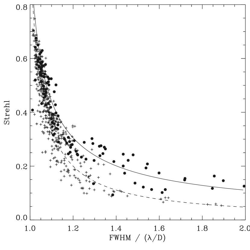
Figure 11: Image Strehl ratio versus normalized FWHM for bright stars (crosses) and faint stars (filled circles).

Figure 11 shows the image Strehl ratio for infrared images versus the normalized FWHM, as defined earlier. In this figure, the crosses refer to guide stars brighter than ${\rm m}_{\rm R}=13.5$ and the filled circles to guide stars fainter than ${\rm m}_{\rm R}=13.5$. These curves show that for bright guide stars, there is a very tight relation between the normalized FWHM and the Strehl ratio, as noted by Tessier (1995). For any given Strehl ratio there is a well–defined normalized FWHM and therefore image shape, whatever the wavelength and the atmospheric conditions. This is expected if one considers the interpretation of AO compensation in terms of the structure function as discussed above. This link between Strehl ratio and FWHM is however difficult to exploit when it comes to determining the Strehl from the FWHM, especially in the domain of high Strehl ${\cal S}>0.3$ where small variations in FWHM correspond to large Strehl variations. Until a more detailed study is carried out to narrow down the Strehl–FWHM relationship, this is at best as a crude indicator of Strehl. Moreover, for higher order systems, the ratio between the diffraction limited core width and the halo width will be larger, and therefore the Strehl–FWHM relationship will be even more bi-modal than the one reported in figure 11, rendering any Strehl determination with this method difficult, or at least very noise sensitive.

Use of faint guide stars modifies the relationship between the Strehl ratio and the normalized FWHM. In terms of modal decomposition, this can be easily understood if one considers that the noise propagation on the correction modes behaves differently than other sources of error. For instance, it is known that noise propagates in a very large part on tip-tilt (especially for curvature systems), and therefore the error on tip-tilt, relative to that of other modes, will be larger when dominated by noise measurement error, broadening the image further, and modifying the Strehl/FWHM relation. Because of insufficient data, we have not been able to investigate how this Strehl–FWHM varies when anisoplanatism comes into play.

5 SCIENTIFIC PROGRAMS

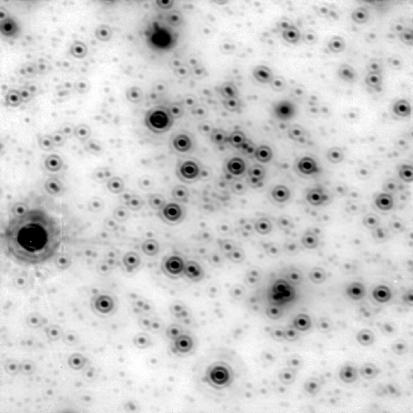
Figure 12: Mosaic image of the galactic center in the $K$ band. The field is 13″ square and the integration time was 15 minutes. North is to the left at an angle of $-$100$\fdg$6 to the vertical, East is up at $-$10$\fdg$6. The brightest objects in the field have been saturated and the gamma correction adjusted on purpose to show the fainter images. Up to 5 diffraction rings are visible around the brightest stars on the original image.

The exploitation of PUEO for regular scientific programs began in August 1996. It already includes surveys of young stars and multiple stars in the Pleiades (Bouvier et al. 1997), imaging of comet Hale-Bopp, the nucleus of M31 (Davidge et al. 1997a), the Galactic center (Davidge et al. 1997b), Seyfert galaxies, QSO host galaxies (Hutchings et al. 1997) and high redshift galaxies. Figure 12 shows the result of a 15 minute observation of the center of our Galaxy in the $K$ band (Rigaut et al. 1997). A ${\rm m}_{\rm R}=14.5$ star approximately 20 arcsec away from the center of the image was used for wavefront sensing. The galactic center was between 1.7 and 2 airmasses during these observations, yet the uncompensated seeing was between 0$\farcs$65 and 0$\farcs$7. In this 13$\times$13 arcsec square image, we have detected more than a thousand stars with a completeness limit of $K\sim$ 16. The faintest objects have $K\sim 19$. The detection is mostly limited by the crowding of the field but, even so, 25 stars per square arcsecond are visible on the original image. Similar, spectacular images on other targets amply demonstrate the potential of adaptive optics for astronomical observations.

6 SUMMARY

The characteristics and performance of the CFHT adaptive optics bonnette have been obtained from an extensive data set taken at wavebands from $B$ to $K$ during 16 nights. These data give many results on both the typical atmospheric conditions encountered on Mauna Kea and on the adaptive compensation. These include:

• Most of the time (80-85%) the observed atmospheric turbulence was well characterized by Kolmogorov turbulence.

• The median value of $r_{0}$ at 500nm was 15.5cm, corresponding to a zenith-corrected seeing disk of FWHM = 0$\farcs$58.

• Analysis of the variation of the observed Strehl ratios as a function of $r_{0}$ indicates that the wavefront correction achieved by PUEO corresponds to full compensation of eight Zernike modes.

• The improvement in the Strehl ratio peaks at $r_{0}\sim$ 50cm (J band in median seeing conditions). The peak intensity of images is improved by a factor twelve at J band and by more than a factor five from $I$ to $K$.

• Images with FWHM$\sim$0$\farcs$1 are common from $I$ to $K$, and are basically diffraction-limited at $H$ and $K$. Significant ($>$2) gains in FWHM are realized at all wavelengths from $B$ to $K$. The maximum gain in FWHM occurs for $r_{0}$ $\sim$ 40 cm.

• A decrease in performance becomes apparent for guide stars fainter than $R$ = 13.5. Strehl ratios are reduced by 50% at $R$ = 15.7 in $K$, 15.0 at $H$, 14.4 at $J$ and $\sim$13 at $R$ under median seeing conditions.

• The observed properties of the PSFs of the compensated images are very stable. We have been able to derive the phase structure function achieved by our system, and proposed an interpretation of this function that explains the global properties of AO compensated images. The phase structure function achieved by the system is, as expected, larger than if only fitting error is considered, largely because of spatial aliasing. One result of this is that the cores of the images are not fully diffraction–limited. The haloes of the images are also affected, but in a very different way, leading to suppressed wings and a lorentzian profile at short wavelengths.

We believe that the operation and the results of this instrument prove that adaptive optics is now a mature technique and can be applied efficiently – in terms of angular resolution, but also in terms of overhead and sensitivity – to astronomy. Our very simple user interface was operated during several nights by astronomers with no a priori knowledge of adaptive optics and proved to be very efficient, robust and reliable. The overhead involved in acquiring astronomical data is comparable to, or even shorter than, that of regular imaging devices since the system automatically achieves perfect guiding and focus. An interactive “AOB performance meter” at http://www.cfht.hawaii.edu/manuals/aob/psf.html provides an estimate of the expected image quality under given seeing conditions for various brightnesses and distances of the guide star. Thanks to the excellent natural seeing at Mauna kea, we can now expect diffraction–limited performance in terms of FWHM, for guide stars as faint as $R$ = 16, offering 0$\farcs$1 resolution to many fields in astronomy, including extragalatic studies.

Table 1: Characteristics of the CFHT Adaptive Optics Bonnette

Subassembly	Characteristic	Description
Optomechanics	Total number of mirrors in science train	5 + 1 beamsplitter (transmission)
	Total number of mirrors in WFS train	9 + 1 beamsplitter (reflection)
	Transmission of Science train	70% (V) excluding beamsplitter
		75% (H), 70% (K) including dichroic
	Input/Output focal ratios	f/8 , f/19.6
	Overall Bonnette dimension	Diameter 120 cm, Thickness 28 cm
	Flexure	$<$10 $\mu{\rm m}$ per hour between WFS
		and science focus
	Optical quality	$\lambda/20$ rms at 0.5 $\mu{\rm m}$  with DM flat
	Instrument clear field of view	90″ diameter
	Atmospheric Dispersion Compensator	Removable
		Designed for zenith distances $<$60°
Wavefront sensor	Type	Curvature
	Number of subapertures	19
	Detectors	APDs (45% peak QE,
		dark current$\sim$ 20e-s-1)
	Field of View	1-2 arcsec depending on optical gain
Deformable mirror	Type	Curvature (+ dedicated Tip-Tilt)
	Number of electrodes	19
	Stroke	$\sim\pm$ 10 $\mu{\rm m}$
	First mechanical resonance	$>$ 2kHz
	Overall dimension	80 mm
	Pupil size on DM	42 mm
	Conjugation	Telescope pupil
	Tip/tilt mirror stroke	$\pm$ 4 arcsec
Control	Sampling/command frequency	Selectable (1000Hz, 500Hz, 250Hz,..)
	Max bandwidth 0dB rejection	105 Hz
	Max bandwidth $-$3dB closed–loop	275 Hz
	Control scheme	Modal, 18 mirror modes controlled
		Closed–loop mode gains optimization
Instrumentation	CCD	2K$\times$2K pixels, 0$\farcs$03 or 0$\farcs$06 pixel-1
	IR imager	NICMOS array, 0$\farcs$034 pixel-1
	Visible integral field spectrograph	Undergoing commissioning

Table 2: Performance Summary For Median Seeing Conditions

Waveband	$V$	$R$	$I$	$J$	$H$	$K$
Wavelength [$\mu{\rm m}$ ]	0.54	0.65	0.83	1.25	1.65	2.23
${\cal S}_{\rm static}$	0.50	0.65	0.75	0.77	0.84	0.93
Median $r_{0}(\lambda)$ [cm]	17	21	28	46	65	93
$D/r_{0}$	21.3	17.1	12.7	7.8	5.6	3.9
Strehl ratio	0.01	0.02	0.05	0.21	0.41	0.61
FWHM [arcsec]	0.24	0.19	0.12	0.095	0.11	0.14
FWHM/($\lambda/D$)	7.6	5.1	2.5	1.34	1.18	1.12
${\rm Gain}_{\rm Strehl}$	4.0	5.0	7.0	12.5	11.6	9.5
${\rm Gain}_{\rm FWHM}$	2.6	3.2	4.8	5.9	5.0	3.6

Figure 1: Optical path of the instrument. The central folding mirrors are on a movable slide, so that the direct and the corrected focus are coincident. A calibration source and target can be inserted at the location of the telescope focus for calibration and testing. The wavefront sensor can be remotely moved to allow selection of a reference star different from the science object.

Figure 2: Distribution of $r_{0}$ values at 500 nm at the Cassegrain focus of the 3.6-m CFH telescope. The solid curve is a fit using a log–normal distribution with mean equal to 15.5 cm and a standard deviation $\sigma=0.13$. This median value corresponds to an observed seeing disk of FWHM = 0$\farcs$67, or 0$\farcs$58 when corrected to the zenith.

Figure 3: An example of the mirror mode coefficient variances: input or uncompensated wavefront (solid line), Kolmogorov fit (diamonds) and the compensated wavefront (triangles and dashed line). The data were normalized for $D/r_{0}=1$ and corrected for noise and spatial aliasing.

Figure 4: Strehl ratio distribution for the $J$, $H$ and $K$ bands. The Strehl values are corrected for the static aberrations of PUEO and the camera (see text).

Figure 5: Strehl ratio, corrected for the optical bench static aberrations, versus the Fried parameter $r_{0}$ at the image wavelength. The bandpasses are noted with different symbols. The lower solid line is the Strehl ratio of the seeing–limited image.

Figure 6: Strehl ratio improvement versus $D/r_{0}$ at the image wavelength. In this and the subsequent two figures, $D/r_{0}$ values for median seeing conditions are shown at the bottom of the figure for wavelength bands from $B$ to $K$.

Figure 7: Gain in FWHM versus $D/r_{0}$ at the image wavelength.

Figure 8: Normalized image FWHM versus $D/r_{0}$ at the image wavelength.

Figure 9: Attenuation of the Strehl ratio compared to the bright guide star case versus the guide star $R$ magnitude for measurements at $H$. Average curves for $J$ and $K$ are also shown.

Figure 10: PUEO characteristic phase structure functions: observed (solid line + error bars), turbulent (dashed line) and high order phase residual alone or “Noll structure function” (dashed-dotted line).

References

- (1) Arsenault, R., Salmon, D.A., Kerr, J., Rigaut, F., Crampton, D. and Grundmann, W.A 1994, SPIE Conf, 2201, 883
- (2) Beuzit, J.-L., Hubin, N., Demailly, L., Gendron E., Gigan, P. et al. 1995, in OSA/ESO topical meeting on Adaptive Optics, ed. M. Cullum (Garching, ESO), p 57
- (3) Bouvier, J., Rigaut, F. and Nadeau, D. 1997, A&A, 323, 139
- (4) Davidge, T.J., Rigaut, F., Doyon, R. and Crampton D. 1997a, A.J., 113, 2094
- (5) Davidge, T.J., Simons, D.A., Rigaut, F., Doyon, R., Becklin, E.E. and Crampton, D. 1997b, A.J., in press
- (6) Ellerbroek, B.L., Van loan, C., Pitsianis, N.P. and Plemmons R.J. 1994, JOSA A, Vol 11, no 11, 2871
- (7) Gaffard, J.-P., Jagourel, P. and Gigan, P. 1994, SPIE Conf, 2201, 688
- (8) Gendron, E. and Léna, P. 1994, A&A, 291, 337
- (9) Graves, J.E. and McKenna, D. 1991, SPIE Conf, 1542, 262
- (10) Graves, J.E., Roddier, F.J., Northcott, M.J. and Anuskiewicz, J. 1994, SPIE Conf, 2201, 502
- (11) Hutchings, J.B., Crampton, D., Morris, S.L., & Steinbring, E. 1997, submitted to PASP
- (12) Lai, O., Arsenault, R., Rigaut F. et al, 1995, in OSA/ESO topical meeting on Adaptive Optics, ed. M. Cullum (Garching, ESO), p. 491
- (13) Noll, R.J. 1976, JOSA, 66 (3), 207
- (14) Racine, R., Salmon, D., Cowley, D. and Sovka, J. 1991, PASP, 103, 1020
- (15) Richardson, E.H. 1994, in NATO ASI Series: Adaptive Optics for Astronomy, eds. D.alloin and J.-M. Mariotti, (Cargése), p. 227
- (16) Rigaut, F., Rousset, G., Kern, P., Fontanella, J.-C., Gaffard, J.-P., Merkle, F. and Léna, P. 1990, A&A, 250, 280
- (17) Rigaut, F., Arsenault, R., Kerr, J., Salmon, D.A., Northcott, M.J., Dutil, Y. and Boyer, C. 1994, SPIE Conf, 2201, 149
- (18) Rigaut, F., Doyon, R., Davidge, T., Crampton, D. and Rouan, D. 1997, submitted to Ap. J.
- (19) Roddier, F.J. 1988, Appl.Opt., 27, 1223
- (20) Roddier, F.J. et al. 1990, SPIE Conf, 1236, 485
- (21) Roddier, F.J., Graves, J.E., McKenna, D. and Northcott, M.J. 1991, SPIE Conf, 1524, 248
- (22) Rousset, G., Fontanella, J.-C., Kern, P. et al. 1990, A&A, 230, L29
- (23) Rousset, G. 1994, in NATO ASI Series: Adaptive Optics for Astronomy, eds. D.alloin and J.-M. Mariotti, (Cargése), p.115
- (24) Tessier, E. 1995, in OSA/ESO topical meeting on Adaptive Optics, ed. M. Cullum (Garching, ESO), p. 465
- (25) Thomas, J., Rigaut, F.J. and Arsenault R. 1997, SPIE Conf, 3126-15
- (26) Véran, J.P., Rigaut, F.J., Rouan, D. and Maitre, H. 1997, JOSA A, 14, 11
- (27) Winker, D.M. 1991, JOSA A, Vol 8, no 10, 1568