IMPLICATIONS OF SPIKES IN THE REDSHIFT DISTRIBUTION OF $z\sim 3$ GALAXIES

Abstract

We address the high peaks found by Steidel et al. (1998) in the redshift distribution of “Lyman-break” objects (LBOs) at redshift $z\simeq 3$. The highest spike represents a relative overdensity of 2.6 in the distribution of LBOs in pixels of comoving size $\sim 10$ $h^{-1}$ Mpc. We examine the likelihood of such a spike in the redshift distribution within a suite of models for the evolution of structure in the Universe, including models with $\Omega=1$ (SCDM and CHDM) and with $\Omega_{0}=0.4-0.5$ ($\Lambda$CDM and OCDM). Using high-resolution dissipationless N-body simulations, we analyze deep pencil-beam surveys from these models in the same way that they are actually observed, identifying LBOs with the most massive dark matter halos. We find that all the models (with SCDM as a marginal exception) have a substantial probability of producing spikes similar to those observed, because the massive halos are much more clumped than the underlying matter – i.e., they are biased. Therefore, the likelihood of such a spike is not a good discriminator among these models. We find in these models that the mean biasing parameter $b$ of LBOs with respect to dark matter varies within a range $b\simeq 2-5$ on a scale of $\sim 10$ $h^{-1}$ Mpc. However, all models show considerable dispersion in their biasing, with the local biasing parameter reaching values as high as ten. We also compute the two-body correlation functions of LBOs predicted in these models. The LBO correlation functions are less steep than galaxies today ($\gamma\approx-1.4$), but show similar or slightly longer correlation lengths.

1. INTRODUCTION

Deep pencil redshift surveys of galaxies can reveal significant information about the clustering of galaxies and the presence of a scale in the structure of the Universe (e.g., Broadhurst et al. 1992, Dekel et al. 1991). Recently, Steidel et al. (1998; hereafter S98) discovered that the redshift distribution of “Lyman-break” objects (LBOs) in a pencil beam reveals a large “spike” in the LBO distribution near $z\simeq 3.1$. This spike corresponds to a fractional overdensity of LBOs of a few hundred percent over a comoving scale of order $\sim 10$ $h^{-1}$ Mpc.

At a first glance, the occurrence of such a dramatic spike seems surprising. This peak suggests substantial nonlinear clustering on rather large scales — scales that are normally considered linear at such early epochs. Indeed, S98 argue that low-$\Omega$ models of the Universe require a biasing parameter $b\simeq 2-4$ to produce such spikes, while models with $\Omega=1$ require even higher biasing. In doing their analysis, S98 attempted a comparison with theoretical scenarios in the “theoretical plane”, corresponding to the matter distribution in real space (as opposed to redshift space) and to epochs of linear evolution. In particular, they translated the data step by step all the way to the linear-fluctuation power spectra, by performing an analytic calculation based on the latest wisdom regarding galaxy “biasing”, redshift distortions, and nonlinear gravitational evolution. The approximations involved in this analysis are somewhat crude, yielding uncertain conclusions.

Subsequently, Bagla (1997) compared the observed spike to the results of pencils in cold dark matter (CDM) numerical simulations. By defining galaxies as regions of high matter density, he found that high spikes were not rare events in such models. The simulations we use for our analysis, unlike those used in Bagla (1997), are of sufficiently high resolution to resolve individual galaxy halos at very high redshift. In the present paper, we identify $z\sim 3$ LBOs with the most massive halos in our simulations at that redshift.

In this paper, we compare the spike in the LBOs of the S98 data to what is expected in four different cosmological models. We do this comparison in the “observational plane”, by observing our numerical simulations just as an observer would. By comparing a suite of different models, we can determine whether the likelihood of a large spike differs greatly among different cosmological models. In relation to the analysis of S98, we examine the biasing of LBO halos compared to the underlying matter. We finally compute the two-point correlation functions of halos in these models. In a Note added, we discuss the relation of our work to other recent papers, and in the Appendix we give a simple analytic treatment of bias that helps explain the results from our simulations.

2. OBSERVATIONAL DATA

Figure 1(a) shows the raw number counts by S98 as a function of redshift, and their estimated selection function.

Figure 1.— Left panel: Redshift histogram from Steidel et al. (1997) showing the number of LBOs in each redshift bin. Also shown is their estimated selection function as a function of redshift. Right panel: Redshift histogram of LBOs divided by the selection function to better reflect the true underlying distribution in redshift space of LBOs. We show only the the 13 central pixels, and instead of the corrected number of LBOs, we plot the relative overdensity of LBOs compared to their average number in a pixel.

The redshift bins, of width $\Delta z=0.04$, represent three-dimensional pixels that are almost rectangular. Their angular dimensions are $\Delta\theta=8^{\prime}.7$ and $\Delta\phi=17^{\prime}.6$. We limit our analysis of the data to the redshift range $2.79<z<3.31$ within which the selection function is higher than 2. This is about 43% of its value at its maximum near $z=3.02$. This cut leaves us with 13 pixels.

Table 1Summary of Parameters for Four Cosmological Models

Model	$z$ range	$N_{\rm pixels}$	Pixel Volume	Mass Threshold	$p$	$q$	$P_{1}$	$P_{2}$	Mean $b$
			($h^{-1}$ Mpc)3	($h^{-1}$ $M_{\odot}$)
SCDM	2.62–2.78	200	1818	$9.0\times 10^{11}$	.005	.025	.06	.02	$2.56\pm 1.04$
CHDM	2.57–2.73	200	1810	$3.1\times 10^{11}$	.035	.070	.37	.18	$4.30\pm 0.77$
$\Lambda$CDM	2.61–2.69	42	5178	$7.3\times 10^{11}$	.024	.048	.27	.10	$3.18\pm 0.37$
OCDM	2.75–2.87	108	2873	$6.9\times 10^{11}$	.028	.056	.31	.13	$3.50\pm 0.84$

Note. — The redshift range covered by the pencils, the number of pixels, the comoving volume of a pixel, and the mass threshold, chosen to reproduce the S98 number density per pixel, are given for each model. Also listed are the fractions $p$ and $q$ of pixels with a fractional overdensity $\delta_{\rm g}$ greater than 2.6 and 1.8, respectively (2.6 and 1.8 are $\delta_{\rm g}$ for the two highest spikes in S98). $P_{1}$ is the probability that at least one pixel out of 13 will have $\delta_{\rm g}$ greater than 2.6, and $P_{2}$ is the probability that at least one additional pixel will have $\delta_{\rm g}$ greater than 1.8. The last column lists the best weighted fit to the local biasing parameter as defined by equation (3) and discussed in Figure 6.

We then multiply the count in each pixel by the inverse of the selection function at the center of the bin (normalized to unity at the maximum, $z=3.02$) and thus obtain a “volume-limited” count in pixels, $N$. We compute the mean corrected count over the pixels, $\bar{N}=4.45$, and record $\delta_{\rm g}=(N-\bar{N})/{\bar{N}}$ in each bin as the data for comparison with theory. This is the only operation we perform on the data; the rest of the analysis is performed on the simulations. Figure 1(b) shows the resulting distribution of $\delta_{\rm g}$. This figure has two high isolated spikes, of $\delta_{\rm g}=2.60$ and $\delta_{\rm g}=1.82$. These spikes seem to be the most interesting features of these data.

The values of $\delta_{\rm g}$ as reported by S98 are somewhat larger than the values quoted here because our definitions of the size of a pixel are somewhat different. Each of our pixels have the angular size of the S98 field and are the length of one their bins in redshift space. Instead, S98 identify “clusters” (defined to be a group of galaxies whose proximity differs from a Poisson distribution), and define the size of their spike by the edges of the cluster that comprises it. This definition of $\delta_{\rm g}$ does not refer to a well-defined scale and it therefore introduces unnecessary complications in the comparison to theory. We therefore prefer to treat the counts in pixels of a fixed volume.

3. SIMULATIONS

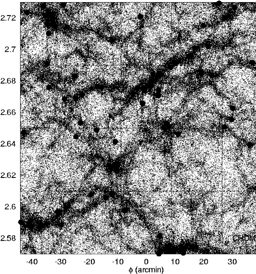
Figure 2.— A slice in redshift space from CHDM at $z\sim 2.65$. The simulation volume has a comoving side 75 $h^{-1}$ Mpc, and the thickness of the slice corresponds to an angle of 8.7 arcminutes, that of the Steidel et al. pencil. The rectangular dotted lines indicate the angular width and the length in redshift space of the Steidel et al. pixels. Shown are randomly sampled particles from the simulation (dots), and a 40% random sample from the halos (solid circles), which matches the observed number density of LBOs. The dark matter distribution shows filamentary structure of moderate amplitude, but several pixels show a high overdensity of halos, consistent with the observed spikes in the distribution of LBOs.

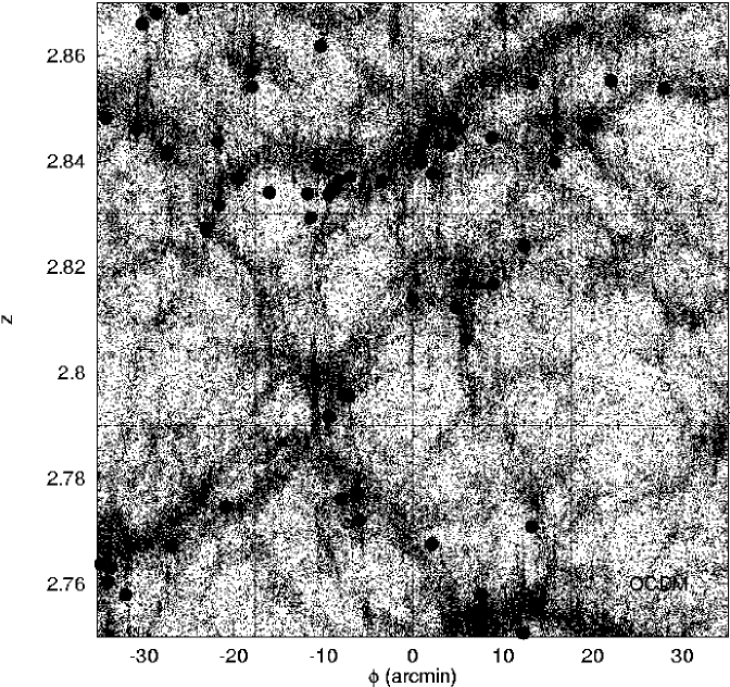
Figure 2. (continued).— The corresponding plot for OCDM at $z\sim 2.81$.

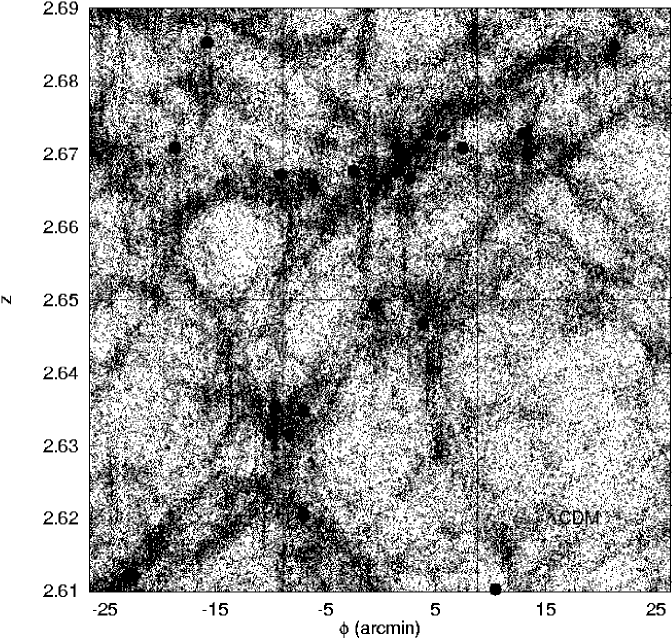
Figure 2. (continued).— The corresponding plot for $\Lambda$CDM  at $z\sim 2.65$. Because of the difference in geometry in $\Lambda$CDM, the pixels are much bigger, and fewer pixels fit in the box.

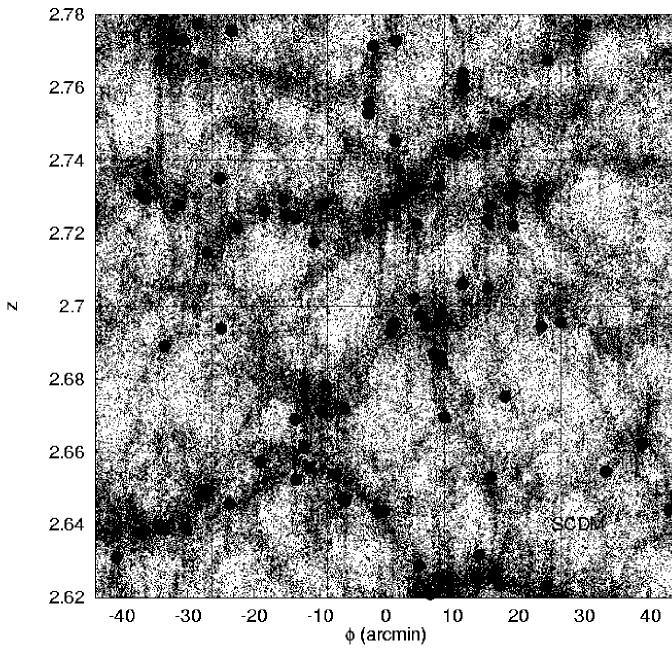
Figure 2. (continued).— The corresponding plot for SCDM at $z\sim 2.70$.

We consider a suite of four different models for the formation of structure in the Universe:

1. One model is standard cold dark matter (SCDM), with density parameter $\Omega=1$, Hubble parameter $h\equiv H_{0}/(100\,\mbox{km s${}^{-1}$ Mpc${}^{-1}$})=0.5$, and a corresponding age of the universe today of $t_{0}=13$ Gyr. The fluctuation amplitude at 8 $h^{-1}$ Mpc is taken to be $\sigma_{8}=0.67$ at $z=0$, in order to approximate the abundance of Abell clusters. Unfortunately, this amplitude is far below the COBE normalization for this model.

2. Another model is the cold+hot dark matter model (CHDM) with $\Omega=1$, $h=0.5$ (thus $t_{0}=13$ Gyr), and $\sigma_{8}=0.72$. We consider two equal-mass neutrino species contributing a total mass density of $\Omega_{\nu}=0.2$. This model is consistent with both cluster and COBE normalization. It is termed CHDM-$2\nu$ in Gross et al. (1997a,b; hereafter G97a,b).

3. Yet another model is the flat cold dark matter model with a nonzero cosmological constant $\Lambda$ ($\Lambda$CDM) and $h=0.6$. Here, the mass density is $\Omega_{0}=0.4$ (relatively high, to obey the constraints on the power spectrum from peculiar velocities in both the Mark III and SFI catalogs, Kolatt & Dekel 1997; Zaroubi et al. 1997; Zehavi et al. 1998), while the cosmological constant corresponds to $\Omega_{\Lambda}=0.6$. In this model $t_{0}=14.5$ Gyr. To simultaneously fit both the cluster abundance and the COBE data, we include a slight tilt to the model, corresponding to a primordial fluctuation spectral index $n_{\rm fluct}=0.90$, which gives $\sigma_{8}=0.88$. This model is called T$\Lambda$CDM in G97a,b.

4. Finally, we consider an open cold dark matter model (OCDM) with $h=0.6$ and $\Omega_{0}=0.5$ (a high value, again, for the same reason as for $\Lambda$CDM); for these parameters, $t_{0}=12.3$ Gyr. Here, $\sigma_{8}=0.77$, consistent with both cluster and COBE normalization.

We simulated the evolution of structure in these models in a purely dissipationless manner. Our approach is based on a parallelized particle-mesh code, which we ran on the Cornell Theory Center SP2. The code is described in Gross (1997, Chapters 2–3); the simulations are discussed in G97a with further discussion of cluster abundance in G97b. These simulations include 57 million cold particles, with an additional 113 million hot particles in the case of CHDM. The simulated box is 75 $h^{-1}$ Mpc in size, giving a mass per cold particle of about $2\times 10^{9}\Omega_{0}$ $h^{-1}$ $M_{\odot}$. A single grid cell is 65 $h^{-1}$ kpc wide in comoving coordinates, corresponding to a physical width of 18 $h^{-1}$ kpc at $z\approx 2.65$.

The simulations were started at different redshifts, reflecting the different fluctuation amplitudes of the various models at high redshift. This means that the earliest redshift at which halos were “observed” in the simulations was somewhat different for each model. The redshifts that we analyze here are $z=2.65$ for CHDM and $\Lambda$CDM, $z=2.70$ for SCDM, and $z=2.81$ for OCDM.

We identify the halos in these simulations using the following procedure: First, we use the density in grid cells to identify candidate halos at the positions of local density maxima and neighboring cells with overdensities $\delta\rho/\rho>50$. Each candidate halo is then iteratively moved to the center of mass of a sphere having a diameter equal to the grid-cell size of 65 $h^{-1}$ kpc. We define the mass of halos as the mass enclosed within a spherical region whose density is sufficient for collapse and virialization (see Gross 1997, Appendix C, for details). At redshift $z=3$, this corresponds to a $\delta\rho/\rho$ of 178 for critical density models, 199 for $\Lambda$CDM, and 203 for OCDM. Finally, we eliminate double counting by excluding smaller halos with centers inside larger halos.

As shown in G97a (Figure 10), we tested this approach by applying it to simulations run with lower spatial resolution and then comparing the resultant halo mass functions. We found that for halo masses used in this paper the grid size had an acceptably small effect. The uncertainty in halo identification is even smaller at $z\sim 3$, where the halos tend to be more isolated and contain less substructure.

We assume that one LBO resides in each massive halo. This assumption is motivated, for example, by a semi-analytic model of galaxy formation in which the brightest objects at $z\sim 3$ are predominantly starbursts in off-center collisions between sub-halo clumps (Somerville, Faber & Primack 1997; Trager et al. 1997; Somerville 1997; Somerville & Primack 1998; Somerville, Primack & Faber 1997). In these simulations there is typically about one such starburst per massive halo at any given time. It would also be true in alternative semi-analytic models in which the LBOs are identified as central halo galaxies (Baugh et al. 1997).

For this paper, we impose a minimum mass for the halos such that the mean number of halos in a pixel is 2.5 times the number of redshifts obtained by S98 per pixel. We do this because S98 measured redshifts for only about 40% of the candidates in their LBO survey. To emulate the data, we therefore randomly select 40% of our halos after setting the mass threshold. This guarantees that each realization of the model matches the observed number of LBOs. The values of the mass threshold we find for each model are listed in Table 1. They range from $M>3.2\times 10^{11}$ $M_{\odot}$ for CHDM to $M>9.0\times 10^{11}$ $M_{\odot}$ for SCDM.

Our procedure of matching the mean number density of LBOs has one important implication. Normally, one expects the abundance of halos of a given mass at a fixed redshift to be a strong function of the model. Some models have earlier galaxy formation than others. However, the exact relation between halos of a given mass and LBOs is not at all clear a priori, especially without the inclusion of gas dynamics and a reasonable model of star formation. Therefore, our elimination of this distinguishing factor allows us to concentrate instead on the variations in the density of objects — especially the spikes.

In Figure 2 we show slices of the underlying mass distribution and a random sample of our identified halos for all four models. These slices have the angular thickness of the S98 pencil; the angular widths of the pencils are indicated in the figure. The comoving sizes of the pixels are different for each model because the fixed angular sizes and redshift interval translate to different comoving scales in different cosmologies. The pencils shown in Figure  2 (a) are only about 30% as long as the observed one. We do not bother to select longer pencils (e.g., at angles to the box sides) because we focus here on single-pixel statistics. One might be concerned about the smaller redshift range represented by an individual simulation volume, or by the difference in redshift between these volumes and the observations, but as we will discuss in the next section, the single-pixel statistics are not strongly dependent on these small changes in redshift.

The figure contains many very noticeable walls and filaments in the underlying mass distribution, not unlike pictures of the galaxy distribution in slices at the current time in the Universe, although the latter would also have massive clusters and larger voids than are visible here. The most massive halos, indicated by filled circles, tend to lie within these sheets and filaments; this concentration of halos into relatively compact regions leads to spikes in the redshift distribution, as we discuss in § 4.

4. STATISTICS OF SPIKES

Using these simulations, we can investigate the statistics of clustering in the observational plane. In particular, we observe pencils in these simulations in redshift space, just as the observers do. The lengths of our pencils are constrained by the box size, and they depend on the model that was simulated. Table 1 lists the redshift extent of the pencils in each model. This corresponds to pencils of length $\Delta z=0.16$ (for CHDM and SCDM), $\Delta z=0.12$ (for OCDM), and $\Delta z=0.08$ (for $\Lambda$CDM). We divide each pencil into 2 to 4 pixels, each identical to the observed pixels. This yields a total of 200 pixels for CHDM and SCDM, 108 for OCDM, and 42 for $\Lambda$CDM. Another reason for variations in the number of pixels that fit in the box is the fact that the fixed angular size of the observed pencils corresponds to different comoving sizes in the different models.

Figure 3.— Fifty pencils (containing 200 independent pixels) laid end to end for the CHDM simulations. Each of the independent pencils is separated by a vertical dotted line, and the pencils are arranged by increasing $\theta$ in groups of increasing $\phi$. The plotted quantity, $\delta_{\rm g}$, for each pixel is the fractional excess of galaxies within each pixel over the average in the realization.

In Figure 3, we show $\delta_{\rm g}$ in the pixels of 50 independent pencils from one random sampling of CHDM stuck together in a row. Each pencil has a length of four pixels, and we separate the pencils with vertical dotted lines. We can afford to deal with pencils that are only four pixels long, because we do not intend to investigate here the effects of correlations between the pixels along a pencil. In particular, we will focus on the question of the probability of finding a single pixel with an overdensity as high as that observed by S98. Since both the observations and the simulations (Figure 3) suggest that the highest peaks are only one pixel wide, this indicates that single pixel statistics may provide a sensitive test for how probable such pencils are in various cosmological models.

Figure 4.— Left panel: A plot of the cumulative distribution of $\delta_{\rm g}$ for the Steidel et al. (1997) data as well as for the halo distribution in the four models considered here. The distribution reflects the relative excess of halos in each pixel. Right panel: The cumulative distribution for the CHDM model compared with the best lognormal fit to that distribution.

For each simulation, we randomly sample 40% of the halos above the threshold five times for each model. We then average over these samplings in order to examine the distribution and statistics of the number of halos in a pixel. In Figure 4 (a) we plot the cumulative distribution of the relative excess in the number of galaxies per pixel, $\delta_{\rm g}$, for each of the four models as well as for the data shown in Figure 1(b). We also plot, in Figure 4(b), the cumulative distribution of $\delta_{\rm g}$ for one of the models, CHDM, compared to the best lognormal fit.

In the CHDM model, the highest pixel has $\delta_{\rm g}=4.8$, almost twice as large as the $\delta_{\rm g}=2.6$ of the highest observed pixel. In fact, there are several pixels in the model with galaxy density higher than the highest observed pixel. The cumulative distribution shows that the probability that the galaxy density contrast in a randomly-chosen pixel of this model will exceed $\delta_{\rm g}=2.6$ is $p=0.035$. The probability $p$ of exceeding this value is given, for each of the models, in Table 1.

If instead of observing one single pixel, one observes $n$ independent pixels, then the probability $P_{1}(n)$ that at least one of the pixels will exceed the threshold $\delta_{\rm g}=2.6$ follows from the binomial distribution:

$$P_{1}(n)=1-(1-p)^{n}\;.$$ (1)

Getting at least one such peak is just one minus the probability of no such peak. Note that equation (1) assumes that there are no correlations among the observed pixels.

In the absence of correlations among the pixels, one could further ask what is the probability $P_{2}(n)$ that one pixel will exceed $\delta_{\rm g}=2.6$ while at least one additional pixel will exceed a certain lower threshold of probability $q$ per pixel. The second-highest pixel in the S98 data has $\delta_{\rm g}=1.8$. The probability $q$ of exceeding this lower threshold for each of the models is also given in Table 1. The probability $P_{2}(n)$ encompasses all possibilities except (a) no pixel above the highest threshold or (b) exactly one pixel above the highest threshold with no additional pixel exceeding the lower threshold. This probability therefore follows directly from the multinomial distribution and is

$$P_{2}(n)=1-(1-p)^{n}-np(1-q)^{n-1}\;.$$ (2)

For $n=13$ randomly chosen pixels, the probability that there will be at least one above $\delta_{\rm g}=2.6$ is 37% for CHDM. The probability of at least one pixel above $\delta_{\rm g}=2.6$ and at least one additional pixel above $\delta_{\rm g}=1.8$ is 18%. These numbers follow from the averaged data for 5 random CHDM selections. In some of the individual selections, the probabilities were as high as $50\%$ and $28\%$. If, instead of randomly sampling 40% of the halos, we set the threshold higher and use all of the halos, $p$ and $q$ are 0.05 and 0.075, which gives $P_{1}=$ 49% and $P_{2}=$ 23%. The other model simulations have slightly lower probabilities, as listed in Table 1.

Probably the biggest surprise here is that all the models except SCDM predict that a large spike at $z\sim 3$ is not a very unusual event. All models except SCDM yield a peak as large as the highest observed by S98 at least 27% of the time, while such a peak occurs in SCDM in 6% of such pencils. It is clear from these statistics that SCDM has less clustering at these high redshifts. It may be that this is due to the shape of the power spectrum $P(k)$, which for SCDM has a shallower slope on the large-$k$ side of the peak than any of the other models. In SCDM the ratio of small-scale to large-scale power is higher than in other models, which results in a more even distribution of galaxies, with more galaxies in the voids (for a visualization showing this, see Brodbeck et al. 1998). The difference in how the LBOs are distributed in the models can be seen clearly by comparing the CHDM and SCDM pixels of Figure 2. In the Appendix, we discuss an analytic formalism that helps to understand the dependence of the spike probability on the shape of the power spectrum. One could further test whether the lack of clustering in SCDM is due to the slope of the power spectrum by looking at simulations of an $\Omega=1$ CDM model with a steeper power spectrum (one which has more large scale power for the same $\sigma_{8}$ normalization), e.g., $\tau CDM$ (see Jenkins et al. 1997).

The model distributions shown in Figure 4 are remarkably similar. One might have thought that low-$\Omega$ models have earlier structure formation and therefore are more likely to show a big spike compared to Einstein-deSitter models with $\Omega=1$. However, there is a competing effect — the fixed angular size of the pixels at a given redshift and the fixed redshift interval mean that the comoving volume of a pixel is larger in open models. The density contrast quoted thus refers to a larger scale, and is therefore expected to be lower. The comoving volume of a pixel is given, for each of the models, in Table 1.

We do not anticipate that there is a significant problem with the fact that we sample at $z\sim 2.65$ rather than the observed $z\sim 3$. In linear theory, the growth of the mass density fluctuations themselves between these two epochs is rather small, less than 10%, and the evolution of the galaxy density fluctuations is expected to be much weaker. In order to demonstrate that, we analyze the CHDM simulation at $z=1$ as if it had the geometry of the simulation at $z=2.65$ (i.e., we take the comoving positions at $z=1$, assume all objects had the same comoving positions at $z=2.65$, and at this earlier time put down pixels of the S98 size); this has the effect of including any evolution in the amplitude of the fluctuations while ignoring changes in geometry. We find that the effect on the statistics is very small: $P_{1}$ = 37% (unchanged from $z=2.65$), and $P_{2}$ = 11% (slightly lower than for $z=2.65$). Thus the main effect in going from lower to higher $z$ is how the pixel geometry is affected, but this effect is rather small in going from $z=2.65$ to 3. For example, if the CHDM simulation (at $z=2.65$) is analyzed as if it were at $z=3.0$, the probabilities become $p=0.042$ (vs. 0.035), and $q=0.083$ (vs. 0.070), which give $P_{1}$ = 43% and $P_{2}$ = 23%. Thus, the likelihood of the spikes in each of the models would be, if anything, slightly increased, had the analysis been done at $z=3$. The general effect we are seeing here is that the massive halos trace the large scale structure and the clustering of these halos evolves rather slowly, while the dark matter meanwhile becomes steadily more clustered – thus the bias of the $10^{12}M_{\odot}$ halos compared to the dark matter will be larger at high redshift.

We have done the same analysis for SCDM at $z=1$. In this case, evolving in redshift from $z=2.70$ to $z=0.93$ (changing the scale factor by a factor of 1.9) is equivalent to changing the amplitude of the model by a factor of 1.9, which is then close to the COBE normalization for SCDM. Again, the effect of this change on the shape of the probability distribution and on the statistics is small: for this case, $P_{1}=0.06$ and $P_{2}=0.01$. One should note that in this analysis and that described in the previous paragraph, we still require that the mean number of LBOs per pixel is the same in each calculation, and set the mass threshold accordingly. This cancels the dominant effects

The angular distribution of halos within high spikes in redshift. The data from the highest spike of Steidel et al. (1997) are shown in panel a, while the other eight panels show two examples of high spikes from each of the simulations. The angular size of the panels correspond to the angular size of the pencil survey of LBOs.

that would have been seen from changes in the evolution or the normalization. Since the normalizations of the four different models at $z=3$ are not different by more than this factor of $\sim 2$, we can conclude that any difference in the spike probabilities between the models are not primarily due to differences in their normalizations. The dependence of the spike probabilities on normalization is discussed further in the Appendix.

One other notable feature of Figure 4 is the fact that, in each of the simulations, between five and ten percent of the pixels are empty, while there are no empty pixels in the data of Figure 1. However, the fact that pencils in other surveyed regions do contain empty pixels (Adelberger, et al. 1998) suggests that this does not represent a significant disagreement between theory and observation.

The spatial distribution of halos on the plane of the sky in each of the models is qualitatively similar to that observed. Figure 4 shows the distribution on the sky of the halos in two “spiky” redshift bins for each model, compared to the data for the highest spike. We can see that halos in the spikes are typically part of a filament or a wall stretching across the pixel. Thus, the spikes in redshift do not correspond to extreme localizations in space, as would be the case for today’s clusters; rather the structures are only slightly localized in angle, and typically only in one dimension. But these “spikes” do end up in rich clusters at the present epoch.

5. BIASING

Another quantity that we can easily measure in our suite of simulations is the biasing relation between the halo and mass-density fluctuations. This will directly connect to the interpretation by S98 of their own observations. In each pixel of the simulations, we have already calculated the density of galactic halos, $\delta_{\rm g}$, and we now compare it to the overdensity of the background matter, $\delta_{\rm m}$, as a direct measure of the biasing on the scale of the pixels. This biasing refers to the specific definition of halos specified in §3, and is particularly dependent on the choice of the halo “edge,” which for our purposes is the radius which encloses a mean density sufficient for collapse by $z\sim 3$.

Figure 5.— Plots of galaxy overdensity in a pixel $\delta_{\rm g}$ versus the dark matter overdensity in the same pixel $\delta_{\rm m}$ for each of the simulated models considered here. The solid line in each curve corresponds to biasing parameter $b=1$. Ignoring underdense regions ($\delta_{\rm m}<0$), we also plot two regression curves to these data. The dotted curve corresponds to a least squares fit, while the dashed curve represents the best fitting straight line when we weight each pixel using the Poisson errors due to the finite number of halos. The values of $b$ and $\sigma$ quoted in the figure correspond to the best slope and its error using the weighted fit.

In Figure 5, we plot for each of the simulations, at the corresponding redshift near $z\sim 3$ (§ 3), the galaxy overdensity in a pixel versus the dark matter overdensity in the same pixel. For each pixel, the local biasing is just the ratio of densities

$$b_{\rm local}=\delta_{\rm g}/\delta_{\rm m}.$$ (3)

To get a measure of the mean biasing of the entire sample at that epoch, we calculate the regression of $\delta_{\rm g}$ upon $\delta_{\rm m}$. Since we are interested primarily in regions that will ultimately collapse, and since the biasing relation is not linear at $\delta_{\rm m}<0$, we use only the positive part of the figures ($\delta_{\rm m}>0$) to calculate the regression. This approach yields the dotted lines. A different approach is to find the best fitting straight line while taking into account the errors (due to Poisson counting) in $\delta_{\rm g}$ within each pixel. This weights the highest $\delta_{\rm g}$ peaks more strongly and leads to the dashed lines in each panel of Figure 5.

Using the weighted measure of mean biasing, we find that the mean biasing parameter $b$ varies from a high of $4.30\pm 1.14$ for CHDM, to a low of $b=2.56\pm 0.52$ for SCDM (Table 1). The error bars we quote correspond to the formal error in the slope fitting. Hence, $b$ is constrained to the range $b\simeq 2-5$ for all models. The low-$\Omega$ models appear less biased than CHDM with $\Omega_{\rm m}=1$, but recall that the volume of a pixel in the low-$\Omega$ models is larger and therefore the biasing measured here refers to a larger scale.

Average biasing does not tell the whole story since there is considerable dispersion in the local biasing parameters, and the selection of high peaks of $\delta_{\rm g}$ clearly biases the local biasing parameter to larger values. For example, in both CHDM and OCDM there are pixels having local biasing greater than 10. In CHDM, most of the regions corresponding to high spikes in the data have a bias of about six, while in the other three models the bias in the regions with high spikes ranges from 3.5-4.5. These values for the bias are similar to the values that S98 found were necessary to get a reasonable probability of large spikes. It was not necessary in our analysis to make all of the assumptions that were necessary for S98 to do the analysis in the theoretical plane, however, which in particular includes the assumption of quasi-linear biasing. Our own simple analytic treatment of the dependence of bias on the shape and normalization of the power spectrum are discussed in the Appendix.

6. CORRELATIONS

Since the probability of a spike in the distribution of LBOs as observed by S98 is not too small for any model considered here (except possibly SCDM), it does not represent a good discriminator between such models. In this comparison, we had to normalize out what might otherwise be the dominant effect — the exponential dependence of the number density of objects on the power-spectrum normalization at high redshift — because it depends on a more accurate identification of halos as LBOs than we were willing to deal with in the present work. Still, there might be hope for better discrimination between models using a statistic that is insensitive to the number density of objects, such as the autocorrelation function.

Figure 6.— Redshift space (left) and real space (right) autocorrelation functions for each model. Functions are calculated in a volume corresponding to all the “pencils” described in §4 for a given model, left in their original positions in the computational box. In calculating the redshift space correlations, each object has had its peculiar comoving velocity along the line of sight added to its coordinate distance, to obtain the observed redshift. The real space data has no such correction, and the dot-dashed line is a comparison to the semi-analytic results for SCDM from Baugh et al. (1997). Our correlation length is very similar to theirs, but our slope seems to be shallower at large separations. Note that the conversion from km s^-1 to comoving $h^{-1}$ Mpc is not merely the Hubble parameter because the distance is measured between two distant objects rather than one distant object and the observer. The correct conversion factor, required to preserve angular separations, is $cz/d$, where $d$ is the coordinate distance to redshift $z$, corresponding to 278$h$ km s^-1 Mpc^-1 for SCDM. Thus the correlation length $r_{0}$, such that $\xi(r_{0})=1$, for the Baugh et al. (1997) curve is $r_{0}$ = 4.0 $h^{-1}$ Mpc, corresponding to $1.1\times 10^{3}$ km s^-1.

Figure 6 shows the three-dimensional redshift-space autocorrelation functions, and also the corresponding real-space autocorrelation functions. In both cases, separations between pairs of LBOs were estimated using the redshift $cz$ as the distance from the observer. Since such a definition must preserve angular separations, the relation between redshift-determined separations $s$ and comoving separations $r$ is

$$s=r\frac{cz}{d(z)},$$ (4)

where $d(z)$ is the coordinate distance to redshift $z$. The ratio $cz/d$ reduces to the Hubble parameter if $z\ll 1$, but for the high redshifts listed in Table 1, it is 281, 278, 206 and 256 $h$ km s^-1 Mpc^-1 for CHDM, SCDM, $\Lambda$CDM and OCDM, respectively.

In calculating the redshift-space correlation function, the velocity along the line of sight is added in a vector fashion. The correlation function is then calculated in the usual manner, by creating a randomly distributed catalog ten times larger than the halo catalog and dividing the number of halo-halo pairs by a tenth of the number of halo-random pairs, as a function of comoving distance in km s^-1. The real-space result is consistent with the semi-analytic estimation of Baugh et al. (1997), with the same correlation length of $\sim$4 $h^{-1}$ Mpc for the SCDM case, but with a flatter slope in our simulations. In Table 2, we give the best fit values of $r_{0}$ (in $h^{-1}$ Mpc) and $\gamma$ for each of the models, in both real and redshift space, for $\xi(r)=(r/r_{0})^{-\gamma}$ fit for $r\leq 5$ $h^{-1}$ Mpc.

Table 2

	Real Space		Redshift Space
Model	$r_{0}$	$\gamma$	$r_{0}$	$\gamma$
	($h^{-1}$ Mpc)		($h^{-1}$ Mpc)
SCDM	3.19	1.69	3.27	1.68
CHDM	4.97	1.55	5.12	1.59
$\Lambda$CDM	6.47	1.48	7.27	1.49
OCDM	4.72	1.52	5.01	1.59

Note. — The best fit value of $r_{0}$ and $\gamma$ are given here for each model. If we set $\gamma=1.8$, to agree with local observations, the values for $r_{0}$ are slightly but not significantly lower.

Interestingly, our correlation length for SCDM at $z\sim 3$ is comparable in comoving coordinates to that of galaxies today, while the other models have somewhat larger correlation lengths; the logarithmic slopes are closer to $\gamma=-1.4$ than the $\gamma\approx-1.8$ observed in galaxy redshift surveys today. Their shallower $\gamma$ may suggest that the LBOs are distributed more like sheets than filaments at $z\sim 3$, and and that they evolve into more filamentary structures with time — or perhaps that they do not evolve into typical bright galaxies at the present epoch. The fact that SCDM has a lower correlation length than the other models perhaps just reflects the well known fact that SCDM, with its power spectrum $P(k)$ having a broad peak, has a matter correlation that becomes negative at smaller separations than the other models we consider, which have $P(k)$ falling faster on the large-$k$ side of the peak (see e.g. Holtzman & Primack 1993 for a discussion of this for the same cosmological models, in the context of the cluster autocorrelation function). Small differences in high-redshift correlation lengths and slopes might help discriminate between models, once enough observational data has been collected to represent a “fair sample” of the universe.

7. CONCLUSIONS

We find that large peaks (“spikes”) in the observed redshift distribution of LBOs within very deep pencils at $z\sim 3$ are a common occurrence among the competing models for the formation of large-scale structure, when LBOs are identified as massive dark matter halos in our high-resolution simulations. Spikes of the sort observed by Steidel et al. (1998) occur frequently in simulations of cold+hot dark matter, open cold dark matter, and a model of CDM containing a cosmological constant, and occasionally in standard cold dark matter.

Note that although our SCDM model has $\sigma_{8}=0.67$ (cluster normalization), increasing the amplitude by a factor of $\sim 2$ (to near-COBE normalization) hardly affected the spike probabilities (as discussed in §4). The fact that such spikes are expected in these models means that the existence of one or more large spikes cannot discriminate among competing models, although additional statistics may begin to do so against SCDM. We speculate that the lower spike probabilities in SCDM, and the fact that SCDM is the model with the least biasing, are a consequence of the shallower slope of its power spectrum. Of course, we have chosen enough halos in all of our simulations to guarantee that the mean number of LBOs at $z\sim 3$ agrees with the observations. More realistic treatment of galaxy formation (or LBOs) may yield different abundances of galaxies at high redshift, and consequently, differing likelihood of large spikes.

We also found that our models give a mean biasing parameter in the range $b\sim 2-5$. This refers to scales of order 10 $h^{-1}$ Mpc at $z\sim 3$, and to a definition of $b$ via unweighted linear regression at $\delta>0$. High-density regions have somewhat higher local biasing values, typically around six for CHDM. In some pixels the local biasing parameter is even greater than 10. Recall that our definition of $b=\delta_{\rm g}/\delta_{\rm m}$ refers to pixels of fixed size while S98 refer to a smaller volume. Note also that our analysis is done in the “observational plane” and it involves the fully non-linear fluctuations in the numbers of LBOs ($\delta_{\rm g}$) and matter ($\delta_{\rm m}$), compared to the analysis in the “theoretical plane” of S98. We find little or no dependence on $\Omega_{0}$ or $\Lambda$, but this is partly due to the differences in pixel volumes with different cosmological parameters. However, our cold plus hot $\Omega=1$ model has the highest mean bias, $\bar{b}=4.3$. It should also be noted that our low-$\Omega_{0}$ models have higher values of $\Omega_{0}$ than the ones that S98 consider, which may be one reason why there is less difference between our models. As discussed in Section 4, the clustering of LBOs (as described by $\delta_{\rm g}$) is not strongly evolving, while the dark matter ($\delta_{\rm m}$) clusters more strongly at low redshift, resulting in a decrease in the bias.

The observation of high spikes is thus consistent with standard cosmology and with straightforward statistical correspondence of LBOs with the most massive dark-matter halos at $z\sim 3$. S98 say in their abstract that “in a cold dark matter scenario the large bias values suggest that individual Lyman-break galaxies are associated with dark halos of mass $M\sim 10^{12}$ $M_{\odot}$, reinforcing the interpretation of these objects as the progenitors of massive galaxies at the present epoch.” Our results imply that the LBOs do have the clustering properties of massive dark matter halos, but it is important to note that this does not necessarily imply that they are the progenitors of present-day massive spheriods. These results are also consistent with a model like that proposed by Somerville, Primack, & Faber (1998) in which although most of the LBOs are found in halos of mass $M\sim 10^{12}$ $M_{\odot}$, the LBOs themselves may be small star-bursting satellites of a central massive object.

The halos identified with LBOs at $z\sim 3$ are distributed on the sky much like those in the highest spike of S98 (see Figure 5), with no evidence of a central concentration. But if one follows the evolution of the regions with the highest spikes, virtually all of them become massive clusters (M$\gtrsim 3\times 10^{14}$ $M_{\odot}$) at the present time. In our CHDM simulation, for example, those halos that correspond to Abell richness $\geq 0$ clusters at $z=0$ have all evolved from regions that were at least as big as the second largest spike found by S98 at $z\sim 3$. This result is consistent with the scenario that the LBOs of $z\sim 3$ now reside in rich clusters of galaxies.

Future observations might affect these conclusions in a variety of ways. It is important to confirm the existence of empty pixels in the galaxy distribution as is predicted by all the models. With full redshift information for all the galaxies in a data set, one will be able to use smaller redshift bins (as S98 did in analyzing their highest peak) and probably draw stronger conclusions. It will be interesting to confirm the predictions of a shallow slope for the correlation function and a correlation length similar to that of nearby galaxies, and to verify whether it is related to sheet-like versus filamentary structure.

Note added: Several papers have appeared on this topic since we submitted this paper; here we briefly comment on how they relate to our work.

Jing & Suto (1998) evaluate the spike probability using simulations of three different cosmological models. Our simulations have comparable force resolution to theirs, but a higher mass resolution by an order of magnitude. They find that a spike the size of the largest one identified by S98 is about twice as probable in SCDM (about one in ten fields) compared to our results (6% probability per field). Their published version agrees with our result that the spike probability in the SCDM model is relatively insensitive to normalization. They also agree with us that the spikes are more probable than SCDM in the low-Omega open and flat models they consider, but these results are not directly comparable to ours since the cosmological parameters of their models are different from ours.

Governato et al. (1998) use N-body simulations, in which they identify galaxies with the help of a semi-analytic model, to investigate the clustering of LBOs. They do not impose the mean density of LBOs, but rather use their semi-analytic model to determine whether a given halo has an object that could be seen in a survey of the type done by S98. The number densities that they find from this method are close to that found by S98. In qualitative agreement with our result, they find that spikes in the distribution of LBOs like the one observed by S98 arise naturally in the two models they consider: SCDM and an open CDM with slightly different parameters than ours. They show that these spikes become rich clusters in the local universe, in agreement with our finding.

Peacock (1998) uses a semi-analytic approximation to determine the bias of LBOs by generating a synthetic redshift histogram and then estimating the variance in cells the size of S98. He again finds that as long as the LBOs are sufficiently biased with respect to the underlying dark matter, most current CDM-type models can account for the data.

Moscardini et al. (1998) discuss theoretical predictions for the number density and correlation function of LBOs. Their semi-analytic predictions for the correlation function are qualitatively similar to ours, and indicate that a better observational determination of the correlation function may be able to discriminate between models.

It is encouraging that there is a general agreement between the results of these different investigations using very different methods, including different $N$-body codes, several different semi-analytic methods, different ways of identifying halos and galaxies, etc. The different papers complement each other and provide a coherent picture with significant confidence.

Giavalisco et al. (1998) calculate the angular correlation function of 871 LBO candidates in five fields of data, and calculate the real-space correlation function using the Limber transform. The correlation lengths that they find are lower than those we find for any of the models we have considered (see Table 2). In future work, we plan to identify LBOs in simulations using semi-analytic models; this may affect the correlation length and power-law index for all of our models.

Appendix A APPENDIX: SPIKE PROBABILITY AND THE POWER SPECTRUM

Table 3

Model	$\sigma_{8}$	$\sigma_{\rm p}$	$M_{\mathrm{h}}$	$\sigma_{\rm h}$	$\nu$	$b$	$\sigma^{\rm h}_{\rm p}$	$\sigma^{\rm h}_{\rm p}$ (sim)
			($h^{-1}$ $M_{\odot}$)
SCDM	0.67	0.19	$1.4\times 10^{12}$	0.73	2.3	3.6	0.68	0.74
CCDM	1.27	0.36	$6.0\times 10^{12}$	1.06	1.6	1.1	0.69	0.70
CHDM	0.72	0.20	$4.0\times 10^{11}$	0.62	2.7	4.8	0.98	0.94

Note. — The values of $\sigma$ have been calculated for these $\Omega=1$ models by using the local power spectrum and then extrapolating back to high redshift by multiplying by the scale factor $1/(1+z)$. For CHDM this is a further approximation, since the power spectrum shape does change slightly over this range of $z$.

The dependence of the spike probability on the cosmological parameters $\Omega$ and $\Lambda$ is qualitatively understood in terms of the fluctuation growth rates and the comoving volumes of the pixels. It is not so obvious, however, why the spike probability is found to be higher in the CHDM model compared to the CDM model, even though they are both of the same Einstein-deSitter cosmology. It is also not obvious a priori why the spike probability is found to be relatively insensitive to the global amplitude (normalization) of fluctuations within a given model, say CDM. We offer here a simple framework in which to understand these trends that we find in the simulations. We provide a heuristic explanation for the dependence of spike probability on the shape and normalization of the power spectrum, involving the issues of halo biasing and abundance (cf. Adelberger et al.1998).

For each model, we characterize the linear power spectrum of fluctuations by $\sigma(M)$, the rms linear density fluctuation in top-hat spheres encompassing a mean mass $M$. Let $M_{\mathrm{h}}$ be the galactic-halo mass threshold chosen to reproduce the correct number density of LBOs; it depends on the cosmological model, but in all cases it corresponds to linear scales of order $\sim 1$ $h^{-1}$ Mpc. Denote $\sigma_{\rm h}\equiv\sigma(M_{\mathrm{h}})$. On the larger scale of the pixels, let $\sigma^{\rm h}_{\rm p}$ and $\sigma_{\rm p}$ be the rms fluctuations for halos and the underlying matter respectively. The pixel scale corresponds to a sphere of a comoving radius $R\simeq 7.6$ $h^{-1}$ Mpc for $\Omega=1$.

One way to define a biasing parameter on the pixel scale is via $b\equiv\sigma^{\rm h}_{\rm p}/\sigma_{\rm p}$. When the halos are identified as rare peaks in a Gaussian field, the biasing parameter is approximated by (Mo & White 1996)

$$b\simeq 1+\frac{\nu^{2}-1}{\delta_{\rm c}},$$ (A1)

where $\nu\equiv\delta_{\rm c}/\sigma_{\rm h}$ measures the “rareness” of the peaks, and $\delta_{\rm c}\simeq 1.686$ is the linear density threshold for collapsed spherical halos. In the case of extremely rare peaks $b\rightarrow\nu/\sigma_{\rm h}$ (Kaiser 1984). Thus,

$$\sigma^{\rm h}_{\rm p}\simeq\frac{\sigma_{\rm p}}{\sigma_{\rm h}}\,\nu+\sigma_{\rm p}(1-\delta_{\rm c}^{-1}).$$ (A2)

The second term is small, $\simeq 0.08$ for SCDM and CHDM, so the interesting dependencies are in the first (Kaiser) term. The ratio $\sigma_{\rm p}/\sigma_{\rm h}$ should clearly depend on the shape of the power spectrum in the sense that a power spectrum with less power on small compared to large scales would tend to lead to a higher $\sigma^{\rm h}_{\rm p}$. This ratio may also depend on normalization indirectly, because $M_{\mathrm{h}}$, and thus $\sigma_{\rm h}$, vary from model to model in order to provide the desired number density of halos. The value of $\nu$ varies from model to model for the same reason, and it could, in principle, depend on shape and normalization.

We can predict for each model the quantities $M_{\mathrm{h}}$ and $\sigma_{\rm h}$ (or $\nu$), and thus $\sigma^{\rm h}_{\rm p}$. One relation between $M_{\mathrm{h}}$ and $\sigma_{\rm h}$ is provided by the power spectrum itself, $\sigma(M)$. An independent constraint on these two quantities is imposed by the fixed number density of halos, enforced to match the observed number density of LBOs. The halo number density is predicted by the Press–Schechter approximation to be

$$n_{\rm h}(M)dM=\sqrt{\frac{2}{\pi}}\left(-\frac{{\rm d}\ln\sigma}{dM}\right)\frac{\bar{\rho}}{M^{2}}\,\nu\,e^{(-\nu^{2}/2)}\,dM.$$ (A3)

For a given power spectrum $\sigma(M)$, we can integrate equation A3 over all masses above the lower threshold $M_{\mathrm{h}}$ and solve for $M_{\mathrm{h}}$ and $\sigma_{\rm h}=\delta_{\rm c}/\nu$. Using equation A1, we can then compute $b$ and $\sigma^{\rm h}_{\rm p}$.

The analytic results for $\sigma^{\rm h}_{\rm p}$ are presented in Table 3 in comparison with the empirical results from the simulations for three models: (1) SCDM, of $\sigma_{8}=0.67$ today; (2) CCDM, a COBE-normalized CDM power spectrum of about twice the amplitude, $\sigma_{8}=1.27$; and (3) our CHDM model, which has a more steeply decreasing power spectrum in the relevant range of wave-numbers. Shown also are the predictions for the matter fluctuations on the pixel scale, $\sigma_{p}$, the analytic solutions for $M_{\mathrm{h}}$ and $\sigma_{\rm h}$, and the corresponding $\nu$ and $b$.

One can see that the predicted halo fluctuations $\sigma^{\rm h}_{\rm p}$, which directly relate to the high-spike probabilities, deviate from the simulation values by only 8% or less. Although the values predicted for $M_{h}$ in the analytic model are systematically higher than those found in the simulations, the effect on the final results are small, and the qualitative trends are clear. The predicted values for the biasing parameter are slightly higher than, but within the errors of, the values given in §5 from the simulations.

What have we learned from the analytic results? The predicted values for $\sigma^{\rm h}_{\rm p}$ in the CDM model are indeed quite insensitive to the normalization. With the higher normalization, there are more halos above any given mass, so the fixed number density $n_{\rm h}$ requires a larger threshold $M_{\mathrm{h}}$. This naturally reduces the increase in $\sigma_{\rm h}$ due to the higher normalization compared to the increase in $\sigma_{\rm p}$ ($\propto\sigma_{8}$), and therefore leads to a larger $\sigma_{\rm p}/\sigma_{\rm h}$. However, this is compensated (in equation A2) by the fact that $\nu$ gets smaller when $M_{h}$ is larger (equation A3).

The spike probability for the steeper, CHDM, spectrum is indeed higher than for SCDM. Here, there are fewer halos above any given mass, so $M_{h}$ must go down in order to keep $n_{\rm h}$ fixed. This naturally corresponds to an increase in $\nu$ (equation A3). Despite the decrease in $M_{h}$, the shape effect forces $\sigma_{h}$ to be smaller in CHDM and therefore $\sigma_{\rm p}/\sigma_{\rm h}$ is larger. The two effects thus both contribute (in equation A2) to the increase in $\sigma^{\rm h}_{\rm p}$.

Indeed, SCDM has long been known to have too much small-scale power to match the observed universe; we now see why such a power spectrum also fails to match the observed clustering of LBOs. A model with a more realistic power spectrum, such as CHDM or $\tau$CDM, will also have a higher, more realistic spike probability.

References

- (1)
- (2) Adelberger, K. L., Steidel, C. C., Giavalisco, M., Dickinson, M., Pettini, M., Kellogg, M. 1998, ApJ, accepted (astro-ph/9804236)
- (3)
- (4) Bagla, J. S., 1997, MNRAS, accepted (astro-ph/9707159, cf. also his astro-ph/9711081)
- (5)
- (6) Baugh, C. M., Cole, S., Frenk, C. S., Lacey, C. G. 1997, ApJ, submitted (astro-ph/9703111)
- (7)
- (8) Brodbeck, D., Hellinger, D., Nolthenius, R., Primack, J. R., & Klypin, A. 1998, ApJ, 495, 1, with accompanying 25 minute videotape
- (9)
- (10) Broadhurst, T. J., Ellis, R. S., Koo, D. C., & Szalay, A. S. 1990, Nature, 343, 726
- (11)
- (12) Dekel, A., Blumenthal, G. R., Primack, J. R., & Stanhill, D. 1992, MNRAS, 257, 715
- (13)
- (14) Governato, F., Baugh, C. M., Frenk, C. S., Cole, S., Lacey, C. G., Quinn, T., & Stadel, J. 1998, Nature, in press (astro-ph/9803030)
- (15)
- (16) Gross, M. A. K., 1997, UCSC Ph.D. dissertation
- (17)
- (18) Gross, M. A. K., Somerville, R. S., Primack, J. R., Holtzman, J., & Klypin, A. A. 1997a, MNRAS, in press (astro-ph/9712142, G97a)
- (19)
- (20) Gross, M. A. K., Somerville, R. S., Primack, J. R., Borgani, S., Girardi, M. 1997b (astro-ph/9711035, G97b)
- (21)
- (22) Holtzman, J. A., & Primack, J. R. 1993, ApJ, 405, 428
- (23)
- (24) Jenkins, A., Frenk, C. S., Pearce, F. R., Thomas, P. A., Colberg, J. M., White, S. D. M., Couchman, H. M. P., Peacock, J. A., Efstathiou, G., Nelson, A. H. 1997, ApJ, in press (astro-ph/9709010)
- (25)
- (26) Jing, Y. P., Suto, Y. 1998, ApJL, 494, L5
- (27)
- (28) Kaiser, N. 1984, ApJL, 284, L9
- (29)
- (30) Kolatt, T. & Dekel, A. 1997 ApJ, 479, 592
- (31)
- (32) Moscardini, L., Coles, P., Lucchin, F., & Matarrese, S. 1998, MNRAS, submitted (astro-ph/9712184)
- (33)
- (34) Peacock, J. Review at the KNAW Colloquium ‘The most distant radio galaxies’, Amsterdam, October 1997, in press (astro-ph/9712068)
- (35)
- (36) Press, W. H., & Schechter, P. 1974, ApJ, 187, 425
- (37)
- (38) Somerville, R. S., 1997, UCSC Ph.D. dissertation
- (39)
- (40) Somerville, R. S., Faber, S. M., & Primack, J. R. 1997, in Proceedings of the Ringberg Workshop on Large Scale Structure, Sept. 23-28, 1996, ed. D. Hamilton (Kluwer Academic Publishers), in press
- (41)
- (42) Somerville, R. S., Primack, J. R. 1998, ApJ, submitted (astro-ph/9802268)
- (43)
- (44) Somerville, R. S., Primack, J. R., & Faber, S. M. 1998, in preparation
- (45)
- (46) Steidel, C.. C., Adelberger, K. L., Dickinson, M., Giavalisco, M., Pettini, M., & Kellogg, M. 1998, ApJ, 492, 428 (S98)
- (47)
- (48) Trager, S. C., Faber, S. M., Dressler, A., & Oemler, A. 1997, ApJ, 485, 92
- (49)
- (50) Zaroubi, S., Zehavi, I., Dekel, A., Hoffman, Y., Kolatt, T. 1997, ApJ, 486, 21
- (51)
- (52) Zehavi, I., Freudling, W. et al.1998, in preparation