The primordial deuterium abundance : problems and prospects

Sergei A. Levshakov^1,2, Fumio Takahara³, and Wilhelm H. Kegel⁴

¹National Astronomical Observatory, Mitaka, Tokyo 181, Japan
²A. F. Ioffe Physico-Technical Institute, 194021 St.Petersburg, Russia
³Department of Earth and Space Science, Faculty of Science, Osaka University, Toyonaka,
Osaka 560, Japan
⁴Institut für Theoretische Physik der Universität Frankfurt am Main, Postfach 11 19 32,
60054 Frankfurt/Main 11, Germany

ABSTRACT

The current status of extragalactic deuterium abundance is discussed using two examples of ‘low’ and ‘high’ D/H measurements. We show that the discordance of these two types of D abundances may be a consequence of the spatial correlations in the stochastic velocity field. Within the framework of the generalized procedure (accounting for such effects) one finds good agreement between different observations and the theoretical predictions for standard big bang nucleosynthesis (SBBN). In particular, we show that the deuterium absorption seen at $z_{a}=2.504$ toward Q 1009+2956 and the H+D Ly$\alpha$ profile observed at $z_{a}=0.701$ toward Q 1718+4807 are compatible with D/H $\sim 4.1-4.6\times 10^{-5}$. This result supports SBBN and, thus, no inhomogeneity is needed. The problem of precise D/H measurements is discussed.

Introduction

The measurement of deuterium abundance at high redshift from absorption spectra of QSOs is the most sensitive test of physical conditions in the early universe just after the era of big bang nucleosynthesis. The standard BBN model predicts strong dependence of the primordial ratio of deuterium to hydrogen nuclei D/H on the cosmological baryon-to-photon ratio $\eta$ and the effective number of light neutrino species $N_{\nu}$ (e.g. Sarkar 1996). According to the basic idea of homogeneity and isotropy of big bang theory the primordial deuterium abundance should not vary in space. One can only expect that the D/H ratio decreases with cosmic time due to conversion of D into ³He and heavier elements in stars.

On the other hand, current measurements of D abundance at high redshift reveal a scatter of the D/H values over approximately one order of magnitude. For instance, recent HST observations of the $z_{a}=0.701$ absorption-line system toward the quasar Q 1718+4807 (Webb et al., 1997a,b) show D/H =$1.8-3.1\times 10^{-4}$. This hydrogen isotopic ratio is significantly higher than that derived from other quasar spectra at $z_{a}=2.504$ [D/H =$1.8-3.5\times 10^{-5}$ by Burles & Tytler, 1996; D/H = $2.9-4.6\times 10^{-5}$ by Levshakov, Kegel & Takahara, 1997 (LKT, hereinafter)], and at $z_{a}=3.572$ [D/H = $1.7-2.9\times 10^{-5}$ by Tytler et al., 1996; D/H $>4\times 10^{-5}$ by Songaila et al., 1997].

The apparent spread of the D/H values makes some authors to assume fluctuations in the baryon-to-photon ratio at the epoch of BBN, i.e. to assume that big-bang nucleosynthesis has occurred inhomogeneously (see e.g. Webb et al., and references cited therein).

Current modeling of the evolution of D/H does not allow to estimate the primordial deuterium abundance with a sufficient accuracy. The depletion factor is strongly model dependent and changes from about 2–3 for the chemical evolution models assuming inflow (e.g. Prantzos 1996, Tosi et al. 1997) up to 10 for the models employing a galactic wind, i.e. outflow (e.g. Scully et al. 1997). This means that both ‘high’ ($\sim 2\times 10^{-4}$) and ‘low’ ($\sim 3\times 10^{-5}$) D/H ratios do not contradict the SBBN prediction if the ISM deuterium abundance of $1.6\times 10^{-5}$ (e.g. Linsky & Wood, 1996) is adopted. Nevertheless, the precise measurements of absolute values of D/H at high redshift are extremely important to check whether BBN does occur inhomogeneously or the basic idea of homogeneity and isotropy is still valid. The fundamental character of this cosmological test requires an unambiguous interpretation of spectral observations.

How accurately can be determined D/H ?

It is well known that the physical parameters derived from spectral data depend on the assumptions made with respect to the line broadening mechanism. For interstellar (intergalactic) absorption lines a ‘non-thermal broadening’ is usually assumed to be caused by a large scale motion of the absorbing gas. The commonly used microturbulent approach considers bulk motions being completely uncorrelated. This yields a symmetrical (Gaussian) distribution of the velocity components parallel to the line of sight, which in turn leads to a symmetrical line profile function being a convolution of a Voigt profile and a Gaussian.

Actually, any turbulent flow exhibits an immanent structure in which the velocities in neighboring volume elements are correlated with each other. Different aspects of the line formation processes in correlated turbulent media have been recently discussed in a series of papers by Levshakov & Kegel (1997, LK hereinafter), Levshakov, Kegel & Mazets (1997, LKM hereinafter), and by LKT.

Once the statistical properties of a turbulent cloud have been specified, the way spectral lines ought to be calculated, depends on the problem considered. Considering emission lines one is dealing with many lines of sight and the observed intensity should closely correspond to the theoretical expectation value (see e.g. Albrecht & Kegel 1987). If, however, one observes the absorption spectrum in the light of a point-like background source, one is dealing with one line of sight only, and the actually observed intensity may deviate substantially from the expectation value (for details see LK and LKM), since averaging along one line of sight only, corresponds to averaging over an incomplete sample. The observed line profile is determined by the velocity distribution along the particular line of sight. For large values of the ratio of the cloud thickness $L$ to the correlation length $l$ the distribution function $p(v)$ for the velocity component along the line of sight approaches the statistical average, which has been assumed to be a Gaussian. For values of $L/l$ of only a few, however, $p(v)$ may deviate substantially from a Gaussian, and is asymmetric in general. This leads to a complex shape of the absorption coefficient for which the assumption of Voigt profiles could be extremely misleading. The actual D/H ratio may turn out to be higher or lower than the value obtained from the Voigt-fitting procedure.

The present paper is primarily aimed at the inverse problem in the analysis of the H+D Ly$\alpha$ absorption observed by Burles & Tytler (1996) and by Webb et al. (1997a,b). The original analysis was performed in the framework of the microturbulent model. Here we make an attempt to re-analyze the observational data on the basis of a more general mesoturbulent model. We consider a cloud with a turbulent velocity field with finite correlation length but of homogeneous (HI-)density and temperature. The velocity field is characterized by its rms amplitude $\sigma_{t}$ and its correlation length $l$. The model is identical to that of LKT. – The objective is to investigate whether the data in question may be interpreted by a unique D/H ratio consistent with the primordial abundances of ⁴He and ⁷Li and theoretical SBBN predictions.

To estimate physical parameters and an appropriate velocity field structure along the line of sight, we used a Reverse Monte Carlo [RMC] technique, i.e. a stochastic optimization algorithm developed to solve optimization problems with a very large number of free parameters (see LKT).

The algorithm requires to define a simulation box for the 5 physical parameters : N(HI), D/H, $T_{kin}$, $\sigma_{t}/v_{th}$, and $L/l$ (here $v_{t}h$ denotes the thermal width of hydrogen lines). – The continuous random function of the coordinate $v(s)$ is represented by its sampled values at equal space intervals $\Delta s$, i.e. by $\{v_{1},v_{2},\dots,v_{k}\}$, the vector of the velocity components parallel to the line of sight at the spatial points $s_{j}$. The total number of intervals depends on the values of $\sigma_{t}/v_{t}h$ and $L/l$, being typically $\sim 100$ for hydrogen absorption lines.

The convergence of the RMC procedure depends on the size of the simulation box which is unknown a priori. If it is too large, the computing time increases considerably, and if it is too small, the required minimum of the objective function may not be reached at all. Therefore the box size must be chosen with some care and should be adjusted to the experimental data. In the next sections we consider two examples of the RMC application.

Deuterium abundance at $z=2.504$ toward Q 1009+2956

We applied at first the RMC procedure to a template H+D Ly$\alpha$ profile which reproduces the Q1009+2956 spectrum with the DI Ly$\alpha$ line seen at $z_{a}=2.504$ (Burles & Tytler 1996). Here we present only a part of our results, the full analysis is given by LKT.

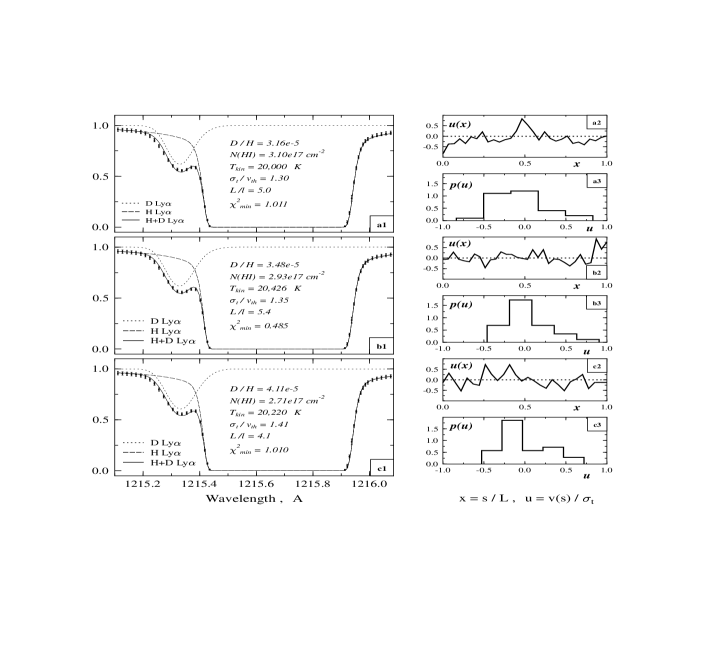
Figure 1: (a1, b1, c1) - A template H+D Ly$\alpha$ profile (dots with error bars) representing the normalized intensities and their uncertainties of the $z=2.504$ system toward Q 1009+2956 in accord with Burles & Tytler (1996). The solid curves show the results of the RMC minimization, whereas the dotted and dashed curves are the separate profiles of DI and HI, respectively. Also shown are the best fitting parameters and the $\chi^{2}$ values obtained for each case.
(a2, b2, c2) - The corresponding individual realizations of the velocity distribution $u(x)$ in units of $\sigma_{t}$.
(a3, b3, c3) - The histograms are the projected velocity distributions $p(u)$.

To simulate real data, we added the experimental uncertainties to the template intensities which were sampled in equidistant bins as shown in Fig. 1 by dots and corresponding error bars. One-component mesoturbulent model with a homogeneous density and temperature was adopted. Adequate profile fits for three different sets of parameters are shown in panels (a1, b1, c1) by solid curves, whereas the individual HI and DI profiles are the dashed and dotted curves, respectively. The estimated parameters (D/H, $N_{\rm HI}$, $T_{kin}$, $\sigma_{t}/v_{th}$, $L/l$) and $\chi^{2}_{min}$ values per degree of freedom are also listed in these panels for each RMC solution.

The essential difference between the results of the two-component microturbulent model adopted by Burles & Tytler and ours lies in the estimation of the hydrodynamical velocities in the $z_{a}=2.504$ absorbing region. It is generally believed that absorption line systems with N(HI)$\sim 10^{17}$ cm^-2 arise in the halos of putative intervening galaxies (e.g. Tytler et al. 1996). The RMC procedure yields $\sigma_{t}\simeq 25$ km s^-1, whereas the two-component model leads to $\sigma_{t}\simeq 2$ km s^-1 which is evidently too low as compared with direct observations of galactic halos at $z>2$ (van Ojik et al. 1997) which show that $\sigma_{t}\simeq 40\pm 15$ km s^-1, if $T_{kin}\simeq 10^{4}$ K.

In this particular absorption system, the study of the H+D Ly$\alpha$ profile yields D/H = $(3.75\pm 0.85)\times 10^{-5}$ which is slightly higher than the value $2.51^{+0.96}_{-0.69}\times 10^{-5}$ found by Burles & Tytler. This difference is, however, very significant because it leads to limits on D/H consistent with other observations discussed below.

Deuterium abundance at $z=0.701$ toward Q 1718+4807

The absorbing material at $z=0.701$ provides an accurate determination of the total hydrogen column density due to the extreme sharpness of the Lyman break measured by the International Ultraviolet Explorer (IUE) satellite (see Webb et al.).

To analyze this system we adopted for the physical parameters the following boundaries (details are given in Levshakov, Kegel & Takahara 1998) :

1.70$\times 10^{17}$ cm${}^{-2}\leq$ N(HI) $\leq 1.78\times 10^{17}$ cm^-2

For D/H we use the range from 3.0$\times 10^{-5}$ to 5.0$\times 10^{-5}$, trying to find a low D/H solution.

For $T_{kin}$ we use the interval $10^{4}-2\times 10^{4}$ K, and, thus, $\sigma_{t}/v_{th}$ may range within 1.3 – 4.3.

For $L/l\gg 1$ the meso- and microturbulent profiles tend to be identical (see LK). Different microturbulent models have been thoroughly investigated by Webb et al., therefore we will consider moderate $L/l$ ratios in the range 1.0 – 5.0.

Figure 2: Observations and RMC fits for Q 1718+4807. (a) – HST/GHRS data (open circles) and calculated profiles for HI (dashed curve), DI (dotted curve) and H+D (solid curve). The spectral resolution corresponds to a FWHM = 0.1 Å. Shown is an acceptable solution of the inverse problem with D/H = $4.111\times 10^{-5}$, N(HI) = $1.768\times 10^{17}$ cm^-2, $T_{kin}=1.51\times 10^{4}$ K, $\sigma_{t}=26$ km s^-1, and $L/l=3.5$ (see Table 1). (b) – residuals $\epsilon$ in units of $\sigma_{noise}$ (see text).
(c) – IUE spectrum (open circles) and fit (solid curve) with a spectral resolution corresponding to a FWHM = 2.95 Å.

Following Webb et al. (1997b), we exclude the Si III line from our analysis of the H+D Ly$\alpha$ profile. As shown by Vidal-Madjar et al. (1996), ‘deducting lines of sight velocity structure for D/H evaluations from ionized species could be extremely misleading’. But we fix $z_{a}({\rm SiIII})=0.701024$ as a more or less arbitrary reference radial velocity at which $v_{j}=0$.

Figure 3: As Fig. 2 but for D/H = $4.755\times 10^{-5}$, N(HI) = $1.759\times 10^{17}$ cm^-2, $T_{kin}=1.75\times 10^{4}$ K, $\sigma_{t}=40$ km s^-1, and $L/l=2.8$ (see Table 1).

The estimated parameters for a few adequate RMC profile fits are listed in Table 1. The derived deuterium abundance $\langle{\rm D/H}\rangle\simeq 4.4\times 10^{-5}$ is about 4–7 times smaller than the limiting values of $1.8-3.1\times 10^{-4}$ found by Webb et al. (1997b) in the microturbulent model excluding the Si III line. To illustrate our results, we show in Figs. 2 and 3 H+D Ly$\alpha$ profiles for the two calculations with the lowest and the highest D abundances found in the mesoturbulent model (D/H = $4.111\times 10^{-5}$ and $4.755\times 10^{-5}$, respectively). They are shown by the solid curve, whereas the open circles give the experimental intensities. The residuals shown in Figs. 2b and 3b by filled circles are normally distributed with zero mean and unit variance.

Figure 4: Probability density functions $p(v)$ for the velocity components parallel to the line of sight for two acceptable RMC solutions shown in Fig.2a (dotted line histogram) and in Fig.3a (solid line histogram). Both are blue-shifted by about $-20$ km s^-1 with respect to $z_{a}({\rm SiIII})$ and have asymmetric shapes.

To control the $v(s)$-configurations estimated by the RMC procedure, we calculated profiles for the higher order Lyman lines and the shape of the Lyman-limit discontinuity and then superposed them to the corresponding part of the Q 1718+4807 spectrum. One expects to find a displacement between the observed and the calculated steep Lyman edge if the velocity field structure is far from the truth. The results are shown in Figs. 2c and 3c where again open circles correspond to the observed intensities and the computed spectra are shown by the solid curves. We do not find any pronounced discordance of calculated and real spectra. On the other hand, the spectral resolution of 2.95 Å (FWHM) is not sufficient to follow a fine velocity field structure within the $z_{a}=0.701$ absorber.

The derived $v(s)$-configurations are not unique. Table 1 demonstrates the spread of the apparent rms turbulent velocities which range from 18 up to 40 km s^-1. It is worthwhile to emphasize once more that the projected velocity distribution function (p.d.f.) may differ considerably from a Gaussian. Fig. 4 shows an example of such distortions caused by a poor statistical sample (i.e. incomplete averaging) of the velocity field distributions for the two cases of the lowest and the highest D/H ratios from Table 1 ($\sigma_{t}=26$ and 40 km s^-1, respectively). Both $p(v)$ distributions are asymmetric. This is the main reason why the absorption in the blue wing of the HI Ly$\alpha$ line may be enhanced without any additional HI interloper(s).

Table 1: Cloud parameters derived from the Ly$\alpha$ profile by the RMC method

N(HI)	D/H	$T_{kin}$	$\sigma_{t}/v^{\rm H}_{th}$	$\sigma_{t}$	$L/l$	$\frac{1}{\nu}\chi^{2}_{min}$
[$10^{17}$ cm-2]		[$10^{4}$ K]		[km s-1]
1.732	4.565	1.41	1.40	22	2.7	1.064
1.739	4.562	1.60	1.10	18	3.9	1.002
1.759	4.755	1.75	2.33	40	2.8	1.106
1.761	4.555	1.46	1.86	29	4.3	1.086
1.768	4.111	1.51	1.61	26	3.5	0.897
1.771	4.442	1.76	1.34	23	3.4	1.162
1.776	4.249	1.62	1.71	28	4.0	1.114

We show that the H+D measurements from two absorption-line systems do not require either a low or a high value of D/H. Both systems at $z=0.701$ toward Q 1718+4807 and at $z=2.504$ toward Q 1009+2956 may be modeled within the framework of the generalized radiative transfer theory with D/H in the range $4.1-4.6\times 10^{-5}$. The fitting procedure leads in this case, however, to asymmetric velocity field distributions. This fact may be used to test the RMC results by additional observations of higher order Lyman lines.

Indeed, if $p(v)$ is asymmetric, this will show up in the profile shapes of the higher order Lyman lines. For example, for the physical parameters listed in Table 1, the effect becomes visible starting from Ly-4 [the Ly-$\alpha$, -$\beta$, -$\gamma$ lines are insensitive to the asymmetry of $p(v)$ due to their high optical depth]. Fig. 5 shows simulated spectra (convolved with a Gaussian instrumental profile of FWHM = 0.1 Å) for Ly-4 and Ly-12 using the same $p(v)$ distributions depicted in Fig. 4 – dotted curves for $\sigma_{t}=26$ km s^-1, and solid curves for $\sigma_{t}=40$ km s^-1. As seen, line shapes may vary depending on the velocity field structure that makes them asymmetric in general. As for microturbulent profiles shown in Fig. 5 by the short dash curves, they remain symmetrical. The higher order Lyman lines may be used unambiguously to constrain the velocity field structure of the absorption system. Therefore high resolution observations of the whole Lyman series become crucial for the D/H measurements.

Figure 5: The HI Ly-4 and Ly-12 mesoturbulent spectra for $\sigma_{t}=40$ km s^-1 (solid curves) and $\sigma_{t}=26$ km s^-1 (dotted curves). The corresponding physical parameters are listed in Table 1. Short dash curves show microturbulent profiles calculated for the mean N(HI) = $1.738\times 10^{17}$ cm^-2 and the mean Doppler parameter $b$(HI) = 25.5 km s^-1 of the data by Webb et al. The spectra are convolved with a Gaussian instrumental profile of FWHM = 0.1 Å.

The revealed mean value of $\langle{\rm D/H}\rangle\simeq 4.4\times 10^{-5}$ corresponds to the mass fraction of ⁴He $Y_{p}\simeq 0.245$, the ⁷Li primordial abundance of $\simeq 2.1\times 10^{-10}$, and $\eta\simeq 4.4\times 10^{-10}$.

The estimated $Y_{p}$ and ⁷Li/H values lie within the measured regions $0.240\leq Y_{p}\leq 0.246$ (Izotov, Thuan, Lipovetsky 1997) and $1.5\times 10^{-10}\leq$ ⁷Li/H $\leq 2.0\times 10^{-10}$ (Bonifacio & Molaro 1997). The measurements of $Y_{p}$ may contain, however, some systematic uncertainties. For instance, Fields et al. (1996) and Olive et al. (1997) give the value $Y_{p}=0.234\pm 0.003({\rm stat.})\pm 0.005({\rm syst.})$ and note that deducing abundances from linestrengths under the usual assumptions about extragalactic HII regions ‘could introduce a significant systematic error’, the magnitude and the distribution of which are ‘not well understood’.

The above baryon-to-photon ratio yields the current baryon density $\Omega_{b}\simeq 0.03$, assuming a Hubble constant ${\rm H}_{0}=70$ km s^-1 Mpc^-1 and the temperature of the cosmic background radiation $T_{CBR}=2.726$ K. This value of $\Omega_{b}$ being larger than the observed density of baryons in stars and hot gas $\Omega_{b,{\rm obs}}\simeq 0.01$ (Fukugita et al. 1996) implies that most baryons are in the hot intergalactic gas.

Conclusion

It is not unlikely that the same spectra may yield different column density estimations. Model dependence of the D/H measurements has been demonstrated within the framework of microturbulent models by Wampler (1996) and on the basis of mesoturbulent models in a series of our papers (see LKT and references therein). Macroscopic motions in QSO absorption systems have been repeatedly confirmed by direct observations (e.g. Songaila et al. 1995). Our analysis shows that such large scale motions may affect the velocity field configuration along the line of sight and the relative positions of the DI and HI lines (Levshakov & Takahara 1996) making their unambiguous interpretation difficult. We stress again that the reliability of the interpretation of the D/H measurements is determined by two factors : ($a$) improvements in the detection equipment and ($b$) advances in the theory of line formation in turbulent media.

The authors are grateful to John Webb for making available the calibrated IUE and HST/GHRS spectra of Q 1718+4807 and acknowledge helpful correspondence and comments by him and Alfred Vidal-Madjar. This work was supported in part by the RFBR grant No. 96-02-16905a.

References

Albrech M. A., Kegel W. H., 1987, A&A, 176, 317
Bonifacio P., Molaro P., 1997, MNRAS, 285, 847
Burles S., Tytler D., 1996, astro-ph/9603069
Fields B. D., Kainulainen K., Olive K. A., Thomas D., 1996, New Astronomy, 1, 77
Fukugita M., Hogan C. J., Peebles P. J. E., 1996, Nature, 381, 489
Izotov Yu., Thuan T. X., Lipovetsky V. A., 1997, ApJS, 108, 1
Levshakov S. A., Takahara F., 1996, Astron. Letters, 22, 438
Levshakov S. A., Kegel W. H., 1997, MNRAS, 288, 787 [LK]
Levshakov S. A., Kegel W. H., Mazets I. E., 1997, MNRAS, 288, 802 [LKM]
Levshakov S. A., Kegel W. H., Takahara F., 1997, MNRAS (submit.), astro-ph/9710122 [LKT]
Levshakov S. A., Kegel W. H., Takahara F., 1998, A&A (submit.)
Linsky J., Wood B. E., 1996, ApJ, 463, 254
Olive K. A., Steigman G., Skillman E. D., 1997, ApJ, 483, 788
Prantzos N., 1996, A&A, 310, 106
Sarkar S., 1996, Rep. Prog. Phys., 59, 1493 Scully S., Cassé M., Olive K. A., Vangioni-Flam E., 1997, ApJ, 476, 521
Songaila A., Hu E. M., Cowie L. L., 1995, Nature, 375, 124
Songaila A., Wampler E. J., Cowie L. L., 1997, Nature, 385, 137
Tosi M., Steigman G., Matteucci F., Chiappini C., 1997, ApJ (submit.), astro-ph/9706114
Tytler D., Fan X.-M., Burles S., 1996, Nature, 381, 207
Vidal-Madjar A., Ferlet R., Lemoine M., 1996, astro-ph/9612020
Wampler E. J., 1996, Nature, 383, 308
Webb J. K., Carswell R. F., Lanzetta K. M., Ferlet R., Lemoine M.,
         Vidal-Madjar A., Bowen D. V., 1997a, Nature, 388, 250
Webb J. K., Carswell R. F., Lanzetta K. M., Ferlet R., Lemoine M.,
         Vidal-Madjar A., 1997b, astro-ph/9710089