Acoustic emission and corrugational instability of shocks modified by strong particle acceleration

Abstract

The effect of particles that undergo strong diffusive-shock-acceleration on the stability of the accelerating shock is investigated. A two-fluid model is employed in which the accelerated particles are treated as a fluid whose effect is incorporated as an additional pressure in the momentum equation. The Dyakov and Kontorovich stability criteria are used in order to study the stability of those steady-state shocks that contain a gas sub-shock. The downstream conditions of the latter are parametrized by the ratio of the upstream acclerated-particles pressure to the total pressure. For some range of values of that parameter, three possible downstream states are possible for each upstream state. It is shown that in that range of parameters the shocks are either corrugationally unstable or lose their energy by spontaneous emission of acoustic as well as entropy-vortex waves.

1 Introduction

Twenty years ago a process, now generally called diffusive shock acceleration, was described whereby a significant part of the kinetic energy flowing into an astrophysical shock could be used to accelerate charged particles (Krymsky, [1977]; Bell 1978a,b; Axford et al., [1977]; Blandford & Ostriker, [1978]). Clearly the reaction of the accelerated particles on the shock dynamics and structure then becomes an important effect. In the intervening years much work has been done, but the problem is a difficult one and many aspects remain open (see reviews by Jones & Ellison, [1991]; Berezhko & Krymsky, [1988]; Blandford & Eichler, [1987]; Völk, [1987]). A significant recent advance is the approximate analytic theory of Malkov ([1997]).

For understandable reasons most of this work has assumed steady, or at least quasi-stationary, shock structures and there has been relatively little work on the question of shock stability. In this paper we apply the classical criteria developed by Dyakov ([1954]) and Kontorovich ([1957]) for the corrugational instability of shock fronts and the spontaneous emission of sound and entropy waves to the simplest model of shocks strongly modified by particle acceleration, the two-fluid model of Drury & Völk ([1981]). While this model has obvious defects (Heavens & Drury, [1988]; Achterberg et al., [1984]) and has clear limitations (Drury et al., [1995]) it has proven to be a useful tool in interpreting numerical studies (Falle & Giddings, [1987]; Jones & Kang, [1990]) when used with appropriate caution.

2 The two-fluid model

The key assumption in the two-fluid model is that the spatial transport of the accelerated particles can be represented by diffusion with a single effective diffusion coefficient. This enables one to integrate over the particle energy spectra and regard the accelerated particles as a second fluid with significant energy density and pressure, but negligible inertia. For historical reasons the accelerated particles are often identified as cosmic rays and the energy density and pressure denoted $E_{\rm C}$ and $P_{\rm C}$,

$$E_{\rm C} = \int 4\pi p^{2}T(p)f(p)dp$$ (1)

$$P_{\rm C} = \int 4\pi p^{2}{pv(p)\over 3}f(p)dp$$ (2)

where $p$ is the magnitude of the accelerated particle momentum, $f(p)$ is the isotropic part of the phase space density, $T(p)$ the associated kinetic energy and $v(p)$ the particle speed.

The two fluid model then consists of the standard hydrodynamical equations for the background gas with density $\rho$, velocity $U$, energy density $E_{\rm G}$ and pressure $P_{\rm G}$ including both pressures in the momentum equation and a diffusive energy flux term with coefficient $\kappa$ in the internal energy equation for the accelerated particle fluid

$${\partial\over\partial t}\rho+\nabla\cdot\left(\rho{\bf U}\right) = 0,$$ (3)

$${\partial\over\partial t}{\bf U}+{\bf U}\cdot\nabla{\bf U}+{1\over\rho}\nabla\left(P_{\rm C}+P_{\rm G}\right) = 0,$$ (4)

$${\partial\over\partial t}P_{\rm G}+{\bf U}\cdot\nabla P_{\rm G}+\gamma_{\rm G}P_{\rm G}\nabla\cdot{\bf U} = 0,$$ (5)

$${\partial\over\partial t}P_{\rm C}+{\bf U}\cdot\nabla P_{\rm C}+\gamma_{\rm C}P_{\rm C}\nabla\cdot{\bf U} = \nabla\left(\kappa\nabla P_{\rm C}\right).$$ (6)

At discontinuities this system has to be replaced by the usual conditions of mass, momentum and energy conservation and continuity of $P_{\rm C}$. The adiabatic exponents $\gamma_{\rm G}$ and $\gamma_{\rm C}$ are defined by

$$P_{\rm G,C}=(\gamma_{\rm G,C}-1)E_{\rm G,C}.$$ (7)

For an ideal monatomic gas $\gamma_{\rm G}=5/3$ and $4/3<\gamma_{\rm C}<5/3$.

The simplicity of the two-fluid model is rather deceptive. All information about the energy (or momentum) spectrum of the accelerated particles has been put in the two closure parameters $\kappa$ and $\gamma_{\rm C}$ and, perhaps not surprisingly, the solutions turn out to depend very sensitively on the assumptions made for these parameters. To some extent this can be overcome by using simple physical models for the spectral evolution to improve the estimates (Duffy et al., [1994]). In addition Malkov & Völk ([1996]) have shown that even in circumstances where the simple two-fluid model is invalid a form of renormalised two-fluid model is applicable.

Our approach in this paper is rather different, We regard the two-fluid equations not as an approximation to some more complicated system, but as the simplest model system (in currently popular terminology a “toy” model) in which we can study the interaction between particle acceleration and shock structure. We note that if the accelerated particles were to have an energy independent diffusion coefficient the two-fluid equations would be exact. Thus the model is physical and does not violate any fundamental physical principles.

All possible stationary shock structures within this model were classified by Drury & Völk, ([1981]). It is interesting to recall one of the concluding remarks in this paper. “Perhaps the most interesting, certainly the most characteristically nonlinear, feature of this model is that under certain circumstances it has three solutions. Whether all are stable and can occur as time asymptotic states in a physically reasonable evolution remains to be studied…”. This paper is a belated answer to this question.

3 Stability criteria for shocks

The study of the stability of shocks was first undertaken by Dyakov, ([1954]). He considered a planar shock wave propagating in an unbounded medium and investigated the evolution of small sinusoidal corrugations of the shock front. Dyakov showed that, under certain conditions, perturbations that are confined to the front’s area grow exponentially with time. This phenomena is termed corrugational instability. Shocks that are corrugationally unstable can only be short-lived because a reorganization of the entire flow will take place on a time-scale of the order of the inverse growth rate.

In addition to the corrugational instability, Dyakov ([1954]) and later Kontorovich ([1957],[1957]) determined the conditions under which small acoustic as well as entropy-vortex perturbations in the form of sinusoidal two dimensional waves can be emitted from the shock front. This phenomenon is termed spontaneous emission. Even though the spontaneously emitted waves do not grow with time, their occurence may eventually render the flow behind the spontaneously emitting shock unstable; this is because the shock’s energy is continuously carried away by the outgoing waves and this finally results in the reorganization of the flow.

Both corrugational instability and spontaneous emission may be treated as resonant reflection of acoustic waves from the shock front where the reflection coefficient of the acoustic waves from the shock is infinite. Wereas historically the reflection coefficient has been calculated in terms of the geometrical parameters of the problem, such as the angles of incidence and reflection, Mond & Rutkevich ([1994]) have recently recast the traditional Dyakov-Kontorovich formulation into a frequency-dependent representation of the reflection coefficient. Such a representation is convenient in solving various boundary value problems such as, for example, investigation of the eigenperturbations between the shock and some other reflecting surface behind it. A further advantage of the frequency-dependent formulation is evident when dissipative effects are taken into account and the relevant frequencies become complex. In this case simple geometric concepts like the angle of incidence are of restricted physical meaning.

The reflection coefficient is calculated by considering an incident acoustic wave as well as reflected acoustic and entropy-vortex waves in the region downstream from the shock of the form

$$\delta f\exp(-i\omega t+i{\bf k}\cdot{\bf r}),$$ (8)

where $\delta f$ is the amplitude of the perturbation of the relevant physical quantity. While $\omega$ and the component of ${\bf k}$ which is parallel to the unperturbed shock front are the same for all the waves involved in the process, the perpendicular component of ${\bf k}$ is determined seperately for each wave according to the appropriate dispersion relation. The upstream perturbations are zero due to the supersonic velocity there. The reflection coefficient is obtained by imposing the continuity of the tangential velocity component as well as the appropriate jump condition of the normal velocity components at the perturbed shock front. Its frequency-dependent representation is given by:

$${\cal R}=-\frac{f(q)-(q^{2}-1)^{1/2}}{f(q)+(q^{2}-1)^{1/2}}$$ (9)

where

$$f(q)=\frac{1-h}{2M_{2}}q-\frac{(1+h)\eta M_{2}}{2q(1-M_{2}^{2})},\;\;\;q=\frac{\omega}{k_{\|}c_{2}(1-M_{2}^{2})^{1/2}},$$ (10)

$M_{2}$ is the downstream Mach number and $\omega$ and $k_{\|}$ are the frequency, and the wave vector component parallel to the shock’s front, of the acoustic as well as of the entropy-vortex waves. As will be seen later, the parameter $h$ plays a crucial role in determining the shock’s stability and is given by

$$h=-v_{2}^{2}{\biggr{(}}\frac{\partial\rho_{2}}{\partial p_{2}}{\biggr{)}}_{\rho_{1},p_{1}},$$ (11)

where $v$, $\rho$ and $p$ are the velocity, density and pressure of the gas, respectively and the subscripts 1 (2) denotes the corresponding values in the upstream (downstream) side of the shock. Thus, $h$ is given in terms of the derivative of the downstream density with respect to the downstream pressure for fixed upstream conditions, i.e., in terms of the slope of the Hugoniot curve.

The problem of stability may be cast now into the following question: under what conditions does the denominator on the right hand side of eq.(9) become zero? The answer is that two families of two dimensional acoustic as well as entropy-vortex waves may give rise to an infinite reflection coefficient under two distinct conditions. The first family of waves is characterized by purely imaginary $\omega$ and purely imaginary $k_{\bot}$ (the wave vector component perpendicular to the shock’s front). Hence, such waves grow exponentially in time and decay exponentially away from the shock. They give rise to the corrugational instability and the conditions for their existence are

$$h<-1,\qquad\hbox{or}\qquad h>1+2M_{2}.$$ (12)

When condition (12) is satisfied, the requirement of an infinite reflection coefficient results in a linear dispersion relation between the growth rate of the instability and the corrugation wavelength, $k_{\|}$.

The second family of waves that can give rise to an infinite reflection coefficient is characterized by real frequencies and real wave vectors. Those waves are the manifestation of spontaneous emission and the condition for their occurence is

$$h_{c}<h<1+2M_{2}$$ (13)

where

$$h_{c}=\frac{1-(1+\eta)M_{2}^{2}}{1+(\eta-1)M_{2}^{2}}$$ (14)

where $\eta=\rho_{2}/\rho_{1}$ is the compression ratio. The implication of condition (13) is that if it is satisfied, there is a one parameter family containing an infinite number of two dimensional acoustic as well as entropy-vortex waves any of which can be spontaneously emitted from the shock front. A linear dispersion relation exists between the frequencies of the spontaneously emitted waves and their parallel wave vectors.

4 Stability of shocks modified by particle acceleration

When conditions (12) and (13) are applied to shocks in an ideal polytropic gas the result is absolute stability against both corrugational instability and spontaneous wave emission. This result is not unexpected and has been well known experimentally since the early days of shock wave research. However, as nonideal processes become progressively more important, the stability properties of the flow may significantly change and the shock may become susceptible to one of the instabilities discussed in the previous section. An example for such occurence has been recently discussed in Mond & Rutkevich ([1997]) where it has been shown that strong ionizing shocks spontaneously emit acoustic waves if their Mach number exceeds a certain value.

Here, the effect of shock accelerated particles on the stability of the accelerating shock is investigated. For that purpose, the two-fluid model discussed in section 2 is employed. Within the framework of this model, a shock is a transition layer between two uniform states, whose length is determined by the mean diffusion coefficient of the particles. Following Drury (1983), it can be shown that the transition layer may either be smooth or contain a sub-shock in the background gas. It is the latter case that will be the focus of the current investigation.

For the purpose of this stability analysis the transition layer that includes the gas sub-shock will be regarded as a single surface of discontinuity. It is this surface that will be called the shock from now on. Such a procedure is admissible if the wavelengths of the investigated perturbations are much larger than the thickness of the transition layer.

4.1 The Hugoniot curve

It is obvious from equations (11)-(13) that the shape of the Hugoniot curve plays a crucial role in determining the stability properties of shocks that propagate into a given uniform state. In order to obtain the Hugoniot curve, the conservation equations that relate the flow variables on both uniform-state-sides of the shock are written in a frame of reference that is moving with the shock’s velocity. For that purpose it is convenient to introduce the following nondimensional variables:

$$\eta=\frac{\rho_{2}}{\rho_{1}},\;\;\;\xi=\frac{P_{{\rm C}1}}{P_{{\rm G}1}+P_{{\rm C}1}},$$ (15)

and

$$\Lambda_{\rm G}=\frac{P_{{\rm G}2}}{P_{{\rm G}1}+P_{{\rm C}1}},\;\;\;\Lambda_{\rm C}=\frac{P_{{\rm C}2}}{P_{{\rm G}1}+P_{{\rm C}1}},$$ (16)

where the subscript 1 (2) denotes the values of the upstream (downstream) corresponding variables. Setting all time derivatives to zero in equations (3)-(6), the following equations are obtained:

$$J^{2}(1-\frac{1}{\eta})-\Lambda_{\rm G}-\Lambda_{\rm C} = -1,$$ (17)

$$\frac{1}{2}J^{2}(1-\frac{1}{\eta^{2}})-\Gamma_{\rm G}\frac{\Lambda_{\rm G}}{\eta}-\Gamma_{\rm C}\frac{\Lambda_{\rm C}}{\eta} = -\theta,$$ (18)

$$J^{2}(\frac{1}{\eta_{a}}-\frac{1}{\eta})+\Lambda_{a}-\Lambda_{\rm G} = 0,$$ (19)

$$\frac{1}{2}J^{2}(\frac{1}{\eta_{a}^{2}}-\frac{1}{\eta^{2}})+\Gamma_{\rm G}(\frac{\Lambda_{a}}{\eta_{a}}-\frac{\Lambda_{\rm G}}{\eta}) = 0,$$ (20)

$$\Lambda_{a} = \eta_{a}^{\gamma_{\rm G}}.$$ (21)

where $\theta=(\Gamma_{\rm G}(1-\xi)+\Gamma_{\rm C}\xi)$, $\Gamma_{G,C}=\gamma_{G,C}/(\gamma_{G,C}-1)$ and $J$ is the normalized mass flux and is given by

$$J^{2}=\frac{\rho_{1}U_{1}^{2}}{P_{{\rm G}1}+P_{{\rm C}1}}.$$ (22)

Equations (17) and (18) represent the momentum and energy conservation, respectively, across the shock while equations (19) and (20) represent the conservation of the background gas momentum and energy across the gas sub-shock. The variables $\Lambda_{a}$ and $\eta_{a}$ are the normalized pressure and density at the foot of the gas sub-shock and are adiabaticaly related to the upstream conditions according to eq. (21).

The solution of the system of equations (17)-(21) result in a one parameter ($\xi$) family of Hugoniot curves. Two such typical curves for $\gamma_{\rm G}=5/3$ and $\gamma_{\rm C}=4/3$ are shown in Fig. 1 for $\xi=0.45$ and in Fig. 2 for $\xi=0.1$. As can be seen in both figures, for small values of $M_{1}$ the Hugoniot curve follows its single-fluid, $\gamma=5/3$ counterpart while for large values of $M_{1}$ it is cosmic-rays dominated as it asymptotically approaches the value of $7$ as predicted for a single-fluid with $\gamma=4/3$. It should be noted, however, that for high enough values of $M_{1}$ no physically acceptable solution of the system of equations (17)-(21) exists which indicates that only a smooth transition layer (without a gas sub-shock) may exist for that range of parameters. The two asymptotic parts of the Hugoniot curve are connected by an intermediate section. As can be seen in Fig. 2, for small values of $\xi$ for some portion of the intermediated section there are three possible downstream states for each upstream state. As will be seen later on, the shock instabilities occur at that intermediate range of parameters.

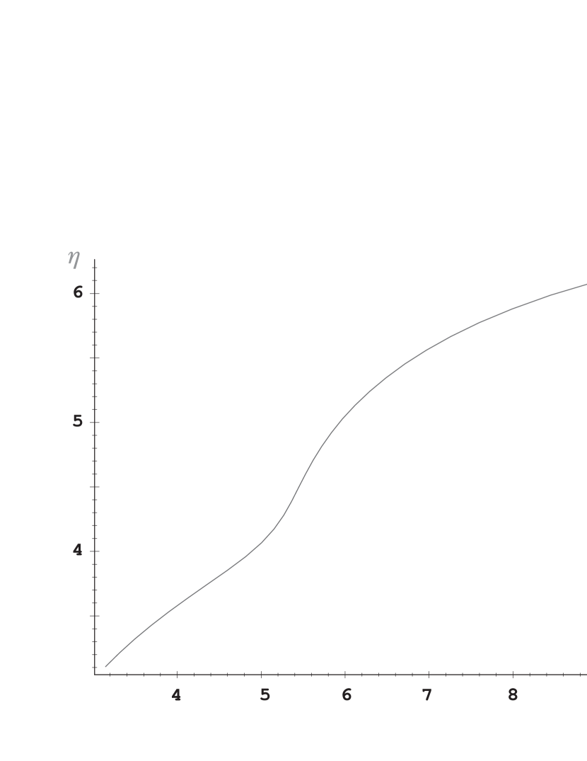
Fig. 1.: The Hugoniot curve for $\xi=0.45$

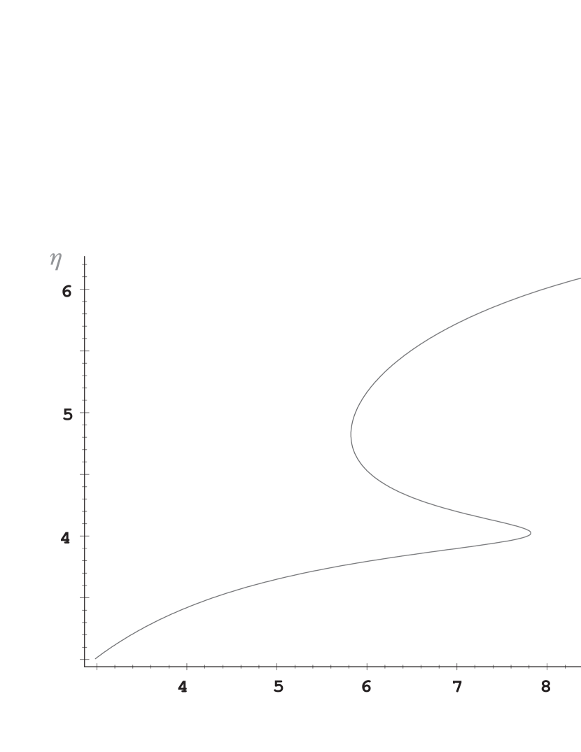
Fig. 2.: The Hugoniot curve for $\xi=0.1$

4.2 The stability analysis

As was discussed in the previous section the concept of a single surface of discontinuity is meaningful only for waves whose wavelengths are much longer than the thickness of the transition layer. In that long wavelength limit the acoustic perturbations in the background gas couple to the accelerated particles and travel at the enhanced speed

$$c^{2}=\frac{\gamma_{\rm G}P_{\rm G}+\gamma_{\rm C}P_{\rm C}}{\rho}$$ (23)

In this case the parameters $h$ and $M_{2}$ that are needed for the calculation of the stability criteria (12) and (13) may be expressed in terms of the nondimensional variables defined in Eqs. (15) and (16) as

$$h=-\frac{J^{2}}{\eta}\frac{\partial\eta}{\partial\Lambda}$$ (24)

where $\Lambda=\Lambda_{\rm G}+\Lambda_{\rm C}$ is the normalized total downstream pressure, and

$$M_{2}^{2}=\frac{J^{2}}{\eta(\Gamma_{\rm G}\Lambda_{\rm G}+\Gamma_{\rm C}\Lambda_{\rm C})}.$$ (25)

The variables $h$ and $M_{2}$ were calculated according to (24) and(25) along the Hugoniot curves and then were used in criteria (12) and (13). The results are shown in Fig.3 and 4 where $h_{c}-h$ is plotted for $\xi=0.45$ and $\xi=0.1$, respectively.

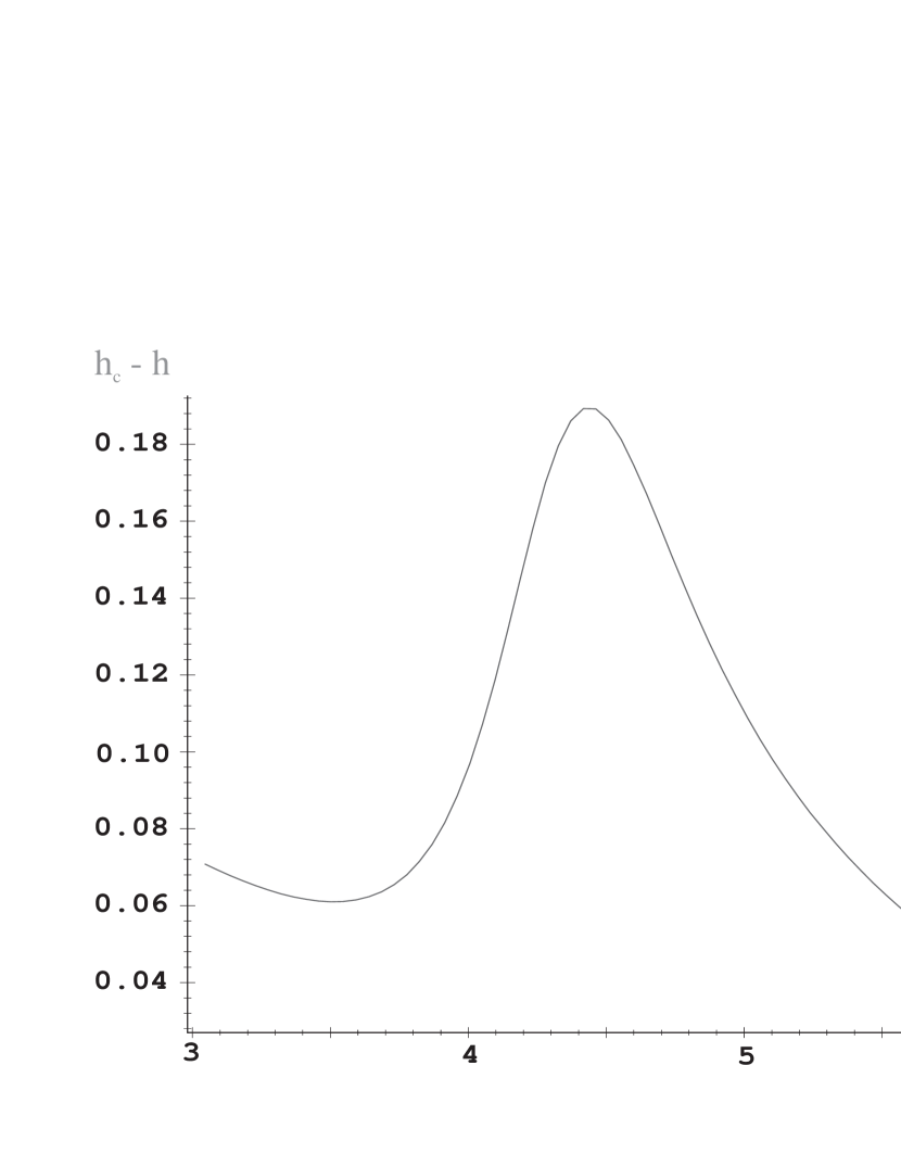
Fig. 3.: The behaviour of $h_{c}-h$ as a function of $\eta$ for $\xi=0.45$

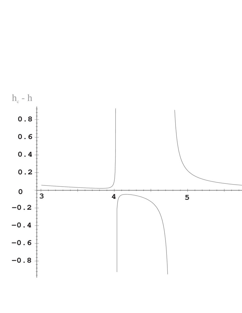
Fig. 4.: The behaviour of $h_{c}-h$ as a function of $\eta$ for $\xi=0.1$

It is obvious that all possible shocks for the $\xi=0.45$ case are stable against both corrugation instability as well as spontaneous emission. This changes however for $\xi=0.1$. In that case there are three possible downstream states for each upstream state at some intermediate section of the Hugoniot curve. According to Fig.4 shocks that belong to the descending part of the intermediate section are unstable under spontaneous acoustic emission. This is so since along that portion of the Hugoniot curve $h$ is positive (see Eq. (24)) while $h_{c}$ remains negative. Furthermore, Fig.2 indicates that the shocks near the “knees” of the Hugoniot curve are corrugationally unstable. An alternative algebraic form for the parameter $h$ is easily seen to be

$$h=-1/\left(1+2(\eta-1){\eta\over U_{1}}{dU_{1}\over d\eta}\right).$$ (26)

This shows that that $h=-1$, indicating the onset of corrugational instability, at precisely those points where the graph of $\eta$ against $U_{1}$ is vertical. A slight further inflection of the graph then allows the denominator to become zero and $h\to\infty$. For such high values of $h$ the dispersion relation that is obtained for the corrugational instability is approximately given by

$$q^{2}=-\frac{\eta M_{2}^{2}}{1-M_{2}^{2}},$$ (27)

so that the growth rate according to the definition in eq. (10) is

$$\sigma=\sqrt{\eta}M_{2}k_{\|}c_{2}.$$ (28)

To complete the stability analysis it should be noted that in the short wavelength limit the acoustic waves decouple from the particles and propagate within the background gas at the gas sound speed $(\gamma_{\rm G}P_{\rm G}/\rho)^{1/2}$. In this limit the acoustic waves propagate through the transition layer and are reflected off the gas sub-shock. Hence, the flow is stable under short wavelength perturbations.

5 The effect of particle diffusion

As was discussed in section 2 the spontaneously emitted waves are marginally stable in the sense that their frequencies are purely real. It is of interest, therefore, to investigate the effects of dissipative mechanisms on the stability of the flow as they give rise to imaginary parts of both the frequencies and the perpendicular wave vector. Hence the question to be asked is whether, under the effects of dissipation, some of the spontaneously emitted eigenperturbations acquire positive imaginary parts of both their eigenfrequencies and their perpendicular wave vectors. This question is still an open one and no general satisfactory answers are available. Furthermore, conflicting claims may be found in the literature with respect to the stabilizing/destabilizing effects of dissipation.

In order to study the effect of the particles dissipation let us reconsider the denominator of the right hand side of Eq.(9). It was tacitly assumed before that the coefficients in that expression (and in particular $M_{2}$) were real. Then the resulting eigenfrequencies were either purely imaginary (corrugation instability) or purely real (spontaneous emission). However, when the effects of particle diffusion are included this ceases to be true and the Mach number, and consequently the frequencies of the spontaneously emitted waves, become complex. Linearizing Eqs. (3)-(7), assuming that the diffusion is small and that $k_{\|}>>k_{\bot}$ results in the following expression for the sound speed

$$c^{2}=c_{0}^{2}(1-i\frac{\gamma_{\rm C}P_{\rm C}}{\gamma_{\rm G}P_{\rm G}+\gamma_{\rm C}P_{\rm C}}x)$$ (29)

where $c_{0}$ is the sound speed in the absence of diffusion and is given by (23) and $x$ is defined by

$$x=\frac{k_{\|}\kappa}{c_{01}}.$$ (30)

With the above modified expression of the sound speed the Mach number is given by

$$M^{2}=M_{0}^{2}(1+i\frac{\gamma_{\rm C}P_{\rm C}}{\gamma_{\rm G}P_{\rm G}+\gamma_{\rm C}P_{\rm C}}x).$$ (31)

Using expression (31) the denominator of the right hand side of Eq. (9) is equated now to zero and solutions for the frequencies are searched such that the corresponding imaginary parts of the perpendicular wave vectors are positive. The sign of the imaginary part of the perpendicular wave vector is checked by using the dispersion relation for the acoustic waves that propagate away from the shock

$$k_{\bot}=\frac{\omega[-M+(1-q^{-2})^{1/2}]}{c(1-M^{2})}.$$ (32)

Using the results for a shock ($M_{1}=4.5$) that belongs to the spontaneous emission regim it is found that the particles dissipation give rise to the damping of the spontaneously emitted waves. As is expected, the damping rate is proportional to $k_{\|}^{2}$ and is much smaller that the corresponding real part of the frequency. Thus, the energy of the shock is continuously being carried away from the shock by the spontaneously emitted waves and is subsequently deposited over a length scale of $1/k_{\bot}$.

6 Discussion

This paper fills a significant gap in the theoretical understanding of the two fluid model by demonstrating what had previously only been conjectured, that in those cases where the model produces multiple solutions the intermediate solution is unstable. It is also, as far as we know, the only case where Dyakov’s criterion for corrugational instability is actually realised in a physically plausible system. In addition to its theoretical interest, we note that the two fluid model is quite extensively used as the basis for numerical studies of particle acceleration effects in astrophysical systems; clearly the knowledge that shock instabilities of the type described here can, indeed must, occur in such simulations is an important piece of information. It will be interesting to see whether similar instabilties are found in more realistic models with momentum dependent diffusion. As we have already noted the two fluid model captures much of the correct physics and is not unphysical. This, together with Malkov’s renormalisation interpretation of the two fluid model, suggests that these effects should also occur in the more complicated models.

This work was carried out while MM was in receipt of a Senior Marie Curie fellowship (contract ERBFMBICT971894) from the European Union under the programme for Training and Mobility of Researchers; MM thanks the school of cosmic physics of the Dublin Institute for Advanced Studies for its friendly and warm hospitality.

References

- 1984 Achterberg, A., Blanford, R.D., Periwal, V. 1984, A&A, 132, 97
- 1977 Axford, W.I., Leer, E., Skadron, G. 1977, Proc. 15th Cosmic Ray Conf., Plovdiv vol 11 (Budapest: Central Research Institute of Physics) pp 132-7
- 1978a Bell, A.R. 1978a, MNRAS, 182, 147
- 1978b Bell, A.R. 1978b, MNRAS, 182, 443
- 1988 Berezhko, E.G, Krymsky, G.F. 1988, Sov. Phys. Usp., 31, 27
- 1978 Blanford, R.D., Ostriker, J.P. 1978, ApJ, 221, L29
- 1987 Blanford, R.D., Eichler, D. 1987, Phys. Reports, 154, 1
- 1983 Drury, L.O’C. 1983, Rep. Prog. Phys., 46, 973
- 1981 Drury, L.O’C., Völk, H.J. 1981, ApJ, 248, 344
- 1995 Drury, L.O’C., Völk, H.J., Berezhko, E.G. 1995, A&A, 299, 222
- 1994 Duffy, P., Drury, L.O’C., Völk, H.J. 1994, A&A, 291, 613
- 1954 Dyakov, S.P. 1954, Zh. Eksp. Teor. Fiz., 27, 288.
- 1987 Falle, S.A.E.G., Giddings, J.R. 1987, MNRAS, 225, 399
- 1988 Heavens, A.F., Drury, L.O’C. 1988, MNRAS, 235,997
- 1991 Jones, F.C., Ellison, D.C. 1991, Space Science Rev., 58, 259
- 1990 Jones, T.W., Kang, H. 1990, ApJ, 363, 499
- 1957 Kontorovich, V.M. 1957, Zh. Eksp. Teor. Fiz., 33, 1525
- 1957 Kontorovich, V.M. 1957, Akust. Zh., 5(3), 314
- 1977 Krymsky, G.F. 1977, Sov. Phys.-Dokl., 23, 327
- 1997 Malkov, M.A. 1997, ApJ, 485, 638
- 1996 Malkov, M.A., Völk, H.J. 1996, ApJ, 473, 347
- 1994 Mond, M., Rutkevich, I. 1994, J. Fluid Mech., 275, 121
- 1997 Mond, M. Rutkevich, I. to appear in Phys. Rev. E
- 1987 Völk, H.J. 1987, Proc. 20th Int. Cosmic Ray Conf., Moscow, 7, 157