The Deuterium Abundance towards QSO 1009+2956

Abstract

We present a measurement of the deuterium to hydrogen ratio (D/H) in a metal-poor absorption system at redshift $z=2.504$ towards the QSO 1009+2956. We apply the new method of Burles & Tytler (1997) to robustly determine D/H in high resolution Ly$\alpha$ forest spectra, and include a constraint on the neutral hydrogen column density determined from the Lyman continuum optical depth in low resolution spectra. We introduce six separate models to measure D/H and to assess the systematic dependence on the assumed underlying parameters. We find that the deuterium absorption feature contains a small amount of contamination from unrelated H I. Including the effects of the contamination, we calculate the 67% confidence interval of D/H in this absorption system, log (D/H) $=-4.40^{+0.06}_{-0.08}$. This measurement agrees with the low measurement by Burles & Tytler (1997) towards Q1937–1009, and the combined value gives the best determination of primordial D/H, log (D/H)${}_{p}=-4.47^{+0.030}_{-0.035}$ or D/H $=3.39\pm 0.25\times 10^{-5}$. Predictions from standard big bang nucleosynthesis (SBBN) give the cosmological baryon to photon ratio, $\eta=5.1\pm 0.3\times 10^{-10}$, and the baryon density in units of the critical density, $\Omega_{b}\,h^{2}=0.019\pm 0.001$, where $H_{0}=100\,h$ km s^-1 Mpc^-1. The measured value of (D/H)_p implies that the primordial abundances of both ⁴He and ⁷Li are high, and consistent with some recent studies. Our two low measurements of primordial D/H also place strong constraints on inhomogeneous models of big bang nucleosynthesis.

1 INTRODUCTION

Measurements of the deuterium-to-hydrogen ratio (D/H) in QSO absorption systems can test current theories of the early universe, in particular, the theory of big bang nucleosynthesis (BBN, c.f. Fuller & Cardall (1996); Schramm & Turner (1997) and references therein). The amount of deuterium produced during the epoch of BBN is very sensitive to the to the cosmological baryon-to-photon ratio, $\eta$ (Reeves et al. (1972); Epstein et al. (1976)). A sample of D/H measurements in QSO absorption systems can establish the primordial abundance ratio of D/H and constrain non-standard models of BBN with limits on the spatial variation of $\eta$ (Jedamzik et al. (1994), Jedamizk & Fuller (1995)). A well constrained primordial D/H value places tight constraints on $\eta$ and gives predicted primordial abundances of the other light elements, which can be compared with current observations to test the paradigm of SBBN (Cardall & Fuller (1996); Hata et al. (1997)).

With high-resolution spectroscopy of distant QSOs, we can measure the deuterium-to-hydrogen ratio (D/H) in select absorption systems which lie along the line of sight (Adams (1976)). High redshift metal-poor QSO absorption systems are ideal sites to infer a primordial value for D/H (Jedamzik & Fuller (1997)). To detect absorption in D-Ly$\alpha$ , the absorption system must have a large hydrogen column density N(H I)$>10^{17}$ cm^-2 and an usually narrow velocity structure (c.f. Tytler & Burles 1997, hereafter TB). We discovered such an absorption system at $z=2.504$ towards the bright QSO 1009+2956 ($z_{em}$ = 2.63, V=16.0). TB performed a preliminary analysis and measurement of D/H in this system. A single consistent absorption model accounted for the H and D absorption in the strongest Lyman lines (Ly$\alpha$ – Ly$\gamma$ ), the metal line profiles of C and Si, and the Lyman continuum break arising from the large H I column. To constrain the hydrogen velocity structure, TB used a two component model for H and D with velocity positions given by the metal line components. TB found log (D/H) = $-4.52\pm 0.08\pm 0.06$ (1$\sigma$ statistical and systematic errors). TB also found that the profile of the deuterium feature suggested contamination from H I , and estimated that D/H is likely lower by 0.08 dex.

Studies of other QSO absorption systems at high redshift give limits on D/H which are consistent with our measurements. Songaila et al. (1994) and Carswell et al. (1994) reported a detection of deuterium in the absorption system at $z=3.32$ towards Q0014+8118. Rugers & Hogan (1996a) reanalyzed the system and measured D/H in two separate components and found D/H = $19\pm 0.5\times 10^{-5}$ in both components. We reobserved Q0014+8118 and found the expected position of D was contaminated with H I absorption, and only an upper limit of D/H $<30\times 10^{-5}$ could be extracted from this system (Tytler et al. 1997). Another system at $z=2.80$ towards Q0014+8118 was analyzed by Rugers & Hogan (1996b). The Ly$\alpha$ absorption feature is the only Lyman line accessible, and we showed that this complex system cannot give any practical constraints on D/H (Tytler et al. 1997). Wampler et al. (1996) find $D/H<15\times 10^{-5}$ at $z=4.672$ towards Q1202$-$0725. Carswell et al. (1996) find a lower limit of D/H $>2\times 10^{-5}$ at $z=3.086$ towards Q0420$-$3851. Webb et al. (1997) recently deduced a D/H value at $z=0.701$ towards the low redshift QSO 1718+4807 using a spectrum obtained with the Hubble Space Telescope (HST). Unlike Q1937–1009 and Q1009+2656, only one H I line was observed, so the velocity structure of the H is not well known. Assuming a single component fit to the Ly$\alpha$ , they find D/H = $20\pm 5\times 10^{-5}$, but this value will remain suggestive unless confirmed with approved HST observations of the high-order Lyman lines. All the above limits on D/H are consistent with our measurements.

The present analysis supersedes that of TB for the following reasons. We have obtained additional spectral data of Q1009+2956, including full coverage of the Lyman series and better quality data above and below the Lyman continuum break. We consider six new absorption models, each with different underlying assumptions about the number of velocity components, free parameters, and exterior constraints. We use the new method to measure D/H in QSO absorption systems described in Burles & Tytler (1997a, hereafter BT). In Sec. 2, we describe the observations and reductions of the spectral data. In Sec. 3, we present the detailed analysis of this absorption system, and discuss the results of the D/H measurement with each of the six new models. in Sec. 4, we combine these results with another measurement of D/H towards Q1937–1009 (Tytler et al. (1996)) to give the tightest constraints on the primordial value of D/H, and calculated the predicted values of $\eta$, $\Omega_{b}$, and the other primordial light element abundances with calculations from SBBN. In Sec. 5, we discuss the implications of low detuerium measurements in two QSO absorption systems and constraints on inhomogeneities during BBN.

2 OBSERVATIONS AND DATA REDUCTION

In this analysis, we use two independent data sets to analyze the absorption system at $z=2.504$ towards Q1009+2956 ($z_{em}$ =2.63, V=16.0). The first data set is a high signal-to-noise ratio (SNR), high-resolution spectrum (FWHM = 8 km s^-1 ) obtained with HIRES at the W. M. Keck 1 10-m Telescope. The high-resolution spectrum fully resolves each absorption line in the Lyman series at $z=2.504$ and allows a detailed analysis of the velocity structure of the absorber, which is required to measure D/H accurately. Six exposures with HIRES, totaling 12.4 hours, are outlined in Table 1. The processing of the CCD images and the extraction of spectra is described in Tytler et al. (1996). Each spectra was normalized to an initial estimate of the quasar continuum by fitting a Legendre polynomial to the unabsorbed regions of the spectra. The spectra were added together, using weights proportional to the SNR to produce a final spectrum.

The second data set is a high SNR, low-resolution spectrum (FWHM = 4 Å) of Q1009+2956, which has been calibrated to an absolute flux scale and has increased sensitivity below 3200 Å, obtained with the Kast Double Spectrograph on the Shane 3-m Telescope at Lick Observatory. We took a total of five hours of data in six separate exposures on the nights of November 28, 1995, and December 15, 1996. The last four exposures used a long (145 arcsec) and wide (9 arcsec) slit to ensure that slit losses were negligible, which gave absolute flux calibration with multiple standard star spectra obtained with the same setup on the same nights. The other spectra were taken with a long narrow (2 arcsec) slit, and were corrected to match the overall flux calibration and smoothed to match the spectral resolution of the wide-slit spectra. The spectra were optimally extracted from the two-dimensional CCD images, after the images were baseline and bias subtracted, and then flat-field corrected. The spectra were set onto a vacuum, heliocentric wavelength scale using images of Ne-Ar and He-Hg-Cd Arc lamps. The final spectrum is shown in Figure 1, and will be referred to as the Lick spectrum throughout this paper.

3 THE MEASUREMENT OF D/H

In this section, we outline the method to measure D/H in the absorption system at $z=2.504$ towards Q1009+2956. A more detailed description of the general method can be found in BT. First, we measure the total hydrogen column density, N(H I)_total , in the D/H absorption system (DHAS). N(H I)_total   represents the sum of the H I column densities in all of the absorbing components in this system. We obtain D/H from models of the Lyman series absorption lines in the HIRES spectrum, which use N(H I)_total  as a constraint.

3.1 Total Hydrogen Column Density

We use the Lick spectrum and the method described in Burles & Tytler (1997b) to measure the Lyman continuum optical depth of the DHAS towards Q1009+2956. To measure the Lyman continuum optical depth, we need to determine the QSO continuum above and below the Lyman break at $912(1+z_{abs})$ Å. We divide the Lick spectrum by the HIRES spectrum to give the unabsorbed continuum level above the break (Burles & Tytler 1997b).

Figure 2 shows the Ly$\alpha$ forest in the Lick spectrum (top panel) and the HIRES spectrum smoothed to the spectral resolution of the Lick spectrum (bottom panel). The crosses in the top panel show the pixels of the Lick spectrum after dividing by the normalized flux level in the smooth HIRES spectrum, and they represent the intrinsic unabsorbed QSO continuum of Q1009+2956.

This continuum of Q1009+2956 shows more structure than Q1937–1009 studied by Burles & Tytler (1997b). The features seen in Figure 2 are likely intrinsic QSO emission lines (Lyman series, Fe III, C III). By removing the intervening absorption features, we can discover and measure new emission lines in high redshift QSO spectra. The slope of the underlying power-law continuum shows a break near 3700 Å(1020 Årest), which was also seen in Q1937–1009, and by Zheng et al. (1997) in the spectra of lower redshift QSOs. We made a linear fit to the continuum blueward of 3700 Å, and the best fit is shown as the straight solid line in Figure 2. We do not use a more complex function because we can not predict the shape of the unabsorbed continuum plus emission lines at $\lambda<3200$ Å. The straight line represents the approximate continuum level in the spectral region below 3700 Å. The standard deviation of the points about the line is 10%, and we use this as the uncertainty of the extrapolated continuum below 3200 Å.

We use the extrapolated continuum to normalize the flux below the Lyman limit, which is shown in Figure 3. Each data point represents the normalized flux in each pixel in the Lick spectrum with 1$\sigma$ error bars. We calculate N(H I)_total in the D/H absorption system using a maximum likelihood method. The model fit includes higher order Lyman lines from absorbers measured at higher wavelengths in the HIRES spectrum, and from a random sampling of the Ly$\alpha$ forest over the region shown in Figure 3. The rest of the Lick spectrum shown in Fig. 3 is consistent with the model constructed from all absorbers at higher redshift ($z>2.00$), and the extra absorption (c.f. at 3155 Å) is accounted for with random Lya lines with redshifts between $1.58<z<1.64$. The drop in flux near 3140 Åis due to a second Lyman limit system at $z=2.43$. We find log[N(H I)_total ] = 17.39 $\pm$ 0.06 cm^-2 (1$\sigma$ error including the 10% continuum uncertainty). The dotted lines in Fig. 3 represent the 1$\sigma$ variation in N(H I)_total .

We compare the measurement of N(H I)_total   to an independent determination using the the highest order Lyman lines in the HIRES spectrum. We apply a simple two component model to the line profiles of Ly-12 to Ly-15. The best fit to the HIRES spectrum gives log N(H I)= 17.35 $\pm$ 0.07 cm^-2 , which is consistent with the Lyman continuum measurement.

In the following analysis we use N(H I)_total as a new constraint on models of the absorption system. The N(H I)in these models must fit the individual Lyman series lines, and be consistent with N(H I)_total .

3.2 Constraining D/H

We use a $\chi^{2}$ minimization routine described by BT, and six new models of the absorption system. As parameters change during the minimization, new model spectra are calculated and compared to the HIRES spectrum in the regions listed in Table 2. Each model includes two types of absorbers: H I lines with enough N(H I)to show D and/or contribute to the total hydrogen column, N(H I)_total   (“main” components). The other type are extra H I lines with low N(H I), which do not contribute significantly to N(H I)_total and do not show D.

All absorbers are modeled as Voigt profiles (Spitzer (1978)). The main components are parameterized by column densities N(D I) and N(H I), temperature, T, turbulent velocity, $b_{tur}$, and redshift, $z$. During the fitting procedure, we assume that D/H is equal in all components, so the column density of D is always given by N(D I) = N(H I) $\times$ (D/H). We model the Lyman lines without using the metal lines, and return to the metal line analysis after the model fitting of the Lyman series is finished. The other H I absorbers, listed in Table 3, are described by three free parameters, column density (N), total velocity dispersion ($b$), and redshift ($z$). The unabsorbed quasar continuum is described by Legendre polynomials of order n, where n is shown in Table 2 for each region. The continuum order is higher in regions with more pixels and higher SNR (i.e. Ly$\alpha$ ) During the initial data reduction, full echelle spectral orders (2048 pixels) were normalized using fifth order Legendre polynomials.

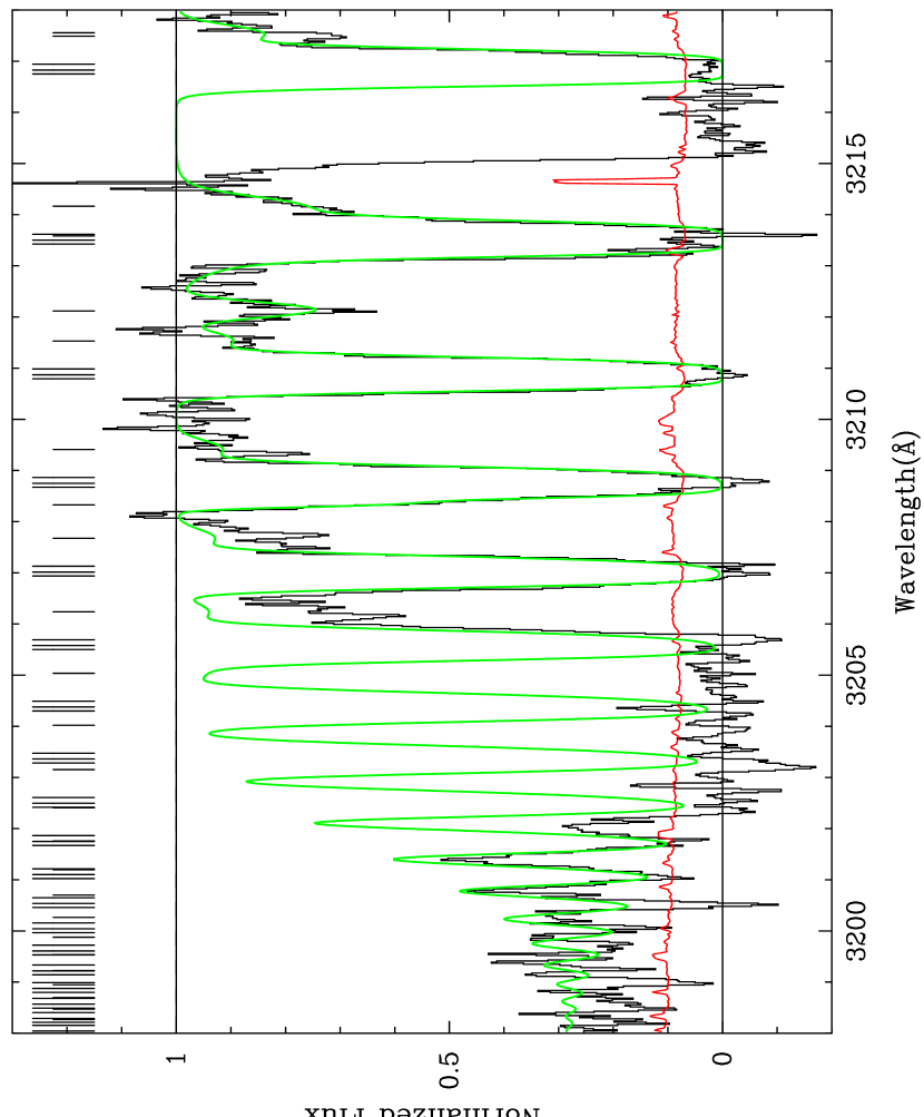
Figure 5: The Lyman limit region of the HIRES spectrum containing Lyman lines of Ly-11 to Ly-24. The histogram represents the observed flux in each 2km s^-1 pixel normalized to the initial estimate of the QSO unabsorbed continuum. The 1$\sigma$ error level in each pix el is represented by the solid line near 0.1. The smooth grey line represents the bes t parameter fit of Model 2. The Lyman line centers are unsaturated above Ly-16, which gives a g ood constraint on the total N(H I)_total in this system from the HIRES spectrum alone.

Figure 4 shows the HIRES spectrum covering the Lyman series lines stacked in velocity space. By stacking the data in velocity space, the alignment of the Lyman absorption lines is evident. The HIRES spectrum spans the entire Lyman series, but we have chosen regions which are free from excessive blending from random Ly$\alpha$ absorption along the line of sight. Fortunately, we can include the majority of high order Lyman lines, Ly-12 and above, which place the tightest constraints on the H I absorption in the main components. The Lyman lines become unsaturated in their line centers at Ly-20 and above. In Figure 5, we show the HIRES spectrum containing these high-order Lyman lines. A large unassociated system, at $z=1.6355$, absorbs all the flux in the region containing the Lyman lines, Ly-16 through Ly-19.

In Figures 4 to 6, the smooth grey line which closely traces the data represents the best fit of Model 2 (discussed below). The entire Lyman series is well fit by the four main H I components (black tick marks). Three main components lie near zero velocity, which is at $z=2.503571$, and the fourth lies redward at $\Delta\,v=66$ km s^-1 . Each main H I component has a corresponding deuterium absorption line (grey tick marks) at a relative velocity of $-81.6$ km s^-1 . The deuterium absorption is significant only in the regions of Ly$\alpha$ and Ly$\beta$ . Figure 6 shows the separate regions listed in Table 2 and used to constrain the model fits. In Figs. 6a and 6b, we also show the individual profiles of the H I and D I absorption features. We start each minimization with the unabsorbed continuum (normalized to unity) shown in Figure 6, then we allow the coefficients of the polynomials to vary during the minimization.

We consider six different models to test the systematic dependence and the sensitivity of the D/H measurement on the underlying assumptions in each model. Each model is constrained by the HIRES data in the spectral regions in Table 2, and N(H I)_total   given by the optical depth of the Lyman continuum absorption in the Lick spectrum. Model 1 has the fewest absorbers, and is the least complex. It includes three main components and allows for free parameters in the continuum specified by the number of free parameters listed in Table 2. The second and third models are identical to Model 1, but they include four and five main components, respectively. The remaining Models (4–6) are identical to Model 2, with one exception each. Model 4 does not use the constraint on N(H I)_total   given by our analysis of the Lick spectrum. By excluding the constraint on N(H I)_total  , we can test how sensitive our measurement of D/H is to the N(H I)_total   constraint. Model 5 does not allow the continuum to vary from the initial continuum estimates. Model 6 includes extra H I absorption to account for possible contamination of the D-Ly$\alpha$ feature.

For each model, we calculate $\chi^{2}_{min}$ for values of D/H from log D/H = $-4.95$ to $-4.00$ in steps of 0.01 dex. We derive confidence levels on D/H by the method of $\Delta\,\chi^{2}$. Table 4 summarizes the results of the $\chi^{2}_{min}$ calculations for all six models. We show the values of D/H which fall in the 95% confidence region, the minimum $\chi^{2}$, along with the overall minimum $\chi^{2}$ for each model and the number of free parameters in each model.

The major results from our analysis with the six different models are shown graphically in Fig. 7, with four different parameters as a function of D/H: $\chi^{2}$, N(H I), $b$(H I), and $\Delta\,v$, where $\Delta\,v/c=\Delta\,z/(1+z_{0})$ and $z_{0}=2.503571$. By presenting the parameters as a function of D/H, we determine their sensitivity to D/H.

Model 1 is very similar to the absorption model analyzed by TB. In the analysis of TB, only spectral coverage of Ly$\alpha$ , Ly$\beta$ , and Ly$\gamma$ was available, so the positions of the hydrogen components were poorly constrained. TB assumed that the two main H I components were matched the velocity positions of two component metal lines, at $\Delta\,v=0,11$ km s^-1 in Fig. 7. The assumption was justified by the predicted deuterium absorption position, but systematic errors could have been introduced. In the present analysis, the positions of the main components are free parameters, and are constrained only by the absorption profiles of the Lyman series. Fig. 7a shows variation of velocity position as a function of D/H. The weaker component (black solid line) does agree with the position of the red metal lines near $\Delta\,v=11$ km s^-1 , but the stronger component at $\Delta\,v=6$ km s^-1 does not match the blue metal lines. The third component at $\Delta\,v=72$ km s^-1 is required to model the absorption in the red wing of the Lyman lines. This component becomes optically thin at Ly-6 and has well constrained parameters that are insensitive to the value of D/H. But the N(H I)from the third component contributes to N(H I)_total , and requires that we include this absorber as a main component. Because its parameters are fairly insensitive to differences between the six different models, we do not display its parameters in the remaining five models in Fig. 7.

Model 2 includes another main H I component, which falls between the two H I components of Model 1 (Fig. 7b), and contains about 10% of the total hydrogen column. This extra component allows a better overall fit to the HIRES spectrum, which gives $\chi^{2}_{min}$ = 906.1 (Table 4). Also, the extra component allows the strongest H I component to move near $\Delta\,v=0$ km s^-1 , but compromises the position of the redward component.

In Fig. 6, we show the individual HIRES spectral regions with the model spectra giving the best fit of Model 2. The model gives a good fit to the data in all of the regions, and the continuum in the best fit model agrees with the initial continuum estimate in all regions except Ly-6. The drop in continuum in the region containing Ly-6 is likely to an additional absorber on the redward side, which was not included in any of the models. The fit is adequate is the Lyman limit region, due to the low SNR in this region, and additional absorbers are not required. The model continuum is constrained by the pixels showing little or no absorption. These pixels are at the edges of the region in Ly$\alpha$ (Fig. 6a), and the continuum is specified by the optical depth in the damping wings, which is proportional to N(H I)_total . The shape of the best fit model continuum suggests that the initial level of continuum was slightly overestimated. The H I and D I absorption profiles are shown as dot-dashed and dashed lines, respectively, in Figs. 6a and 6b (Ly$\alpha$ and Ly$\beta$ ). Both profiles represent the total absorption of the three strongest components in Model 2 (components shown in Fig. 7b). Notice that the deuterium profile is asymmetric, with a steeper blue wing, like the metal lines. This qualitatively validates the TB assumption that the main H components are at similar velocities to the metals, although an exact quantitative match is not realized.

Model 3 incorporates a fifth hydrogen component (Fig 7c.), and all parameters adjust to the new additional absorber. Unlike Model 2, the absorbers shift away from $\Delta\,v=0$ km s^-1 . The total hydrogen column is split between four main components the velocity dispersions are much lower in three of the components. There is an improvement in $\chi^{2}$, but not as significant as the addition of the fourth component. Model 3 does not represent the whole system as well as Model 2, and the $\chi^{2}$ improvement does not warrant the addition of more more than four components. Model 2 is less complex than Model 3, gives a similar fit to the data, and agrees better with the metal lines.

In Model 4, we exclude the constraint on N(H I)_total given by the Lick spectrum, and constrain the absorption model by the HIRES spectrum only. The results are shown in Fig 7d. and are very similar to Fig. 7b, which we expect but Model 2 and 4 are identical with the exception of the relaxed N(H I)_total constraint. So the HIRES data alone give the same results for D/H as those using both spectra, although the uncertainties are larger for Model 4. We find that the N(H I)_total constraint is useful, but not crucial, since the high order Lyman lines approach unsaturation and give strong constraints on N(H I)_total independently.

Model 5 demonstrates the systematic offset introduced by not allowing free parameters in the unabsorbed continuum level. The best fits from the four previous models suggest that the continuum level across the Ly$\alpha$ feature was overestimated. Therefore Model 5 requires a higher N(H I)_total to increase the damping wings of Ly$\alpha$ , and shifts the confidence regions to lower values of D/H. We also point out that of all six models, the uncertainties in D/H are the smallest in Model 5. This is certainly not because of the $\chi^{2}_{min}$ of Model 5, which is the highest of any model. The smaller uncertainty on D/H is due to the smaller the number of free parameters and not because Model 5 gives a better fit to the data.

Model 6 includes an additional H I absorber, but unlike previous models, introduces this absorption at the position of the deuterium feature. This unrelated H I absorbs flux at or near the position of D I , and represents contamination of D. Model 6 gives the best fit to data out of all six models. The two strongest H I components show the best match to positions of the metal lines in the 95% confidence region. In Figures 8a and 8b, we show the regions of Ly$\alpha$ and Ly$\beta$ , respectively, for the best fit of parameters of Model 6.

Our main conclusion is that all six models give consistent confidence ranges for D/H. In Fig. 9, we display the 95% confidence intervals on D/H calculated in each of the six models. The first four models show that D/H is not very sensitive to the number of main components nor the inclusion of the constraint on N(H I)_total . These first four models are consistent with log (D/H) = $-4.36\pm 0.09$ (95% confidence). Model 5 shows that free parameters in the continua do affect D/H and the overall fit to the Lyman lines. Model 6 shows that contamination of the D is likely, and below we discuss the implications of this result in detail.

3.3 Contamination

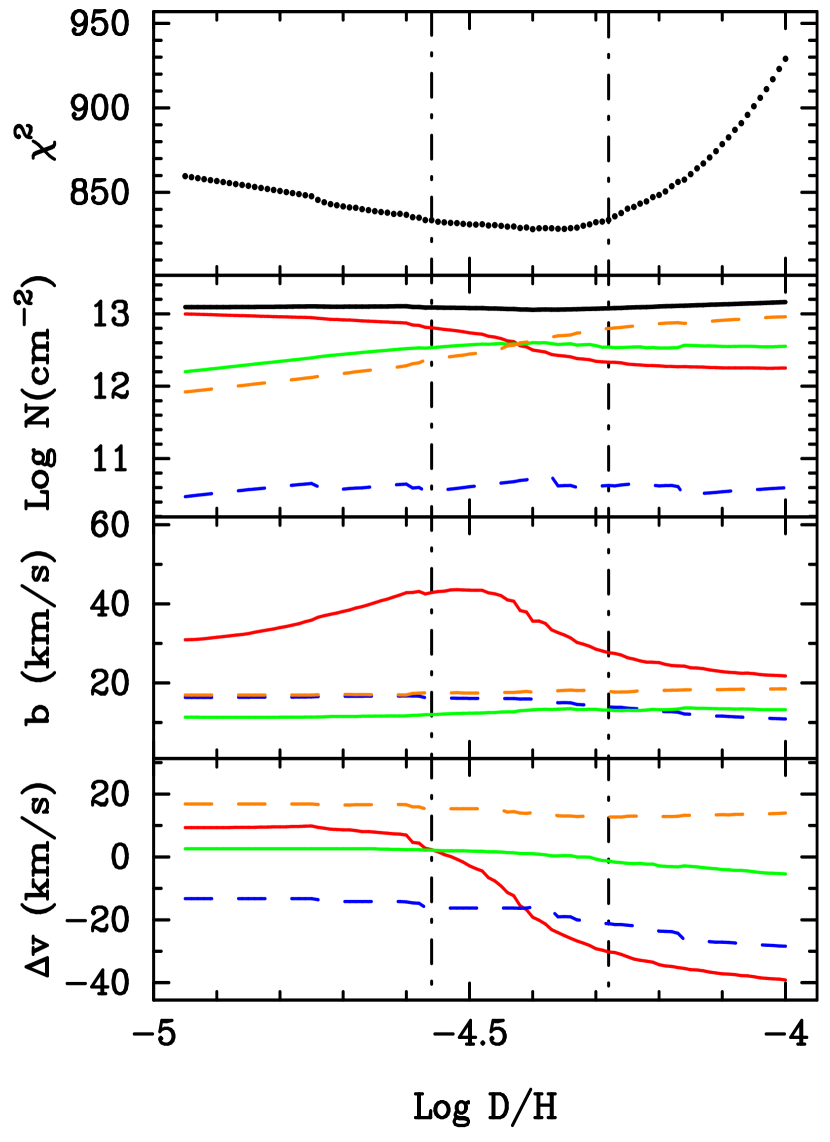
Figure 10: Results of the fitting procedure of Model 6. The parameters are displayed as in Fig. 7f, but represent the components of D I and the contaminating H I absorber.

We have shown that the introduction of contamination with a single H I absorber gives a dramatic improvement in the best fit to the data. The improved $\chi^{2}_{min}$ of Model 6 with respect to all other models is the first indication that contamination is likely. The effects of the contaminating hydrogen absorber can be seen in Figure 10. Figure 10 is similar to Fig. 7, but in Fig. 10 we show the parameters for three D I components and the contaminating H I absorber in Model 6. The column densities show that the contaminating N(H I)adjusts to maintain a total column of log N $=13.1$ cm^-2 for the whole deuterium feature for low values of D/H (log (D/H) $<-4.4$). This effectively relaxes the constraint on the main H I components, and allows for a better fit to all Lyman lines for low values of D/H. With this constraint relaxed, the H I components give best fit velocity positions which are very similar to the metal line velocities, and gives more weight to the existence of contamination. The contaminating absorber also relaxes the constraints on the continuum level at Ly$\alpha$ , and gives a better match between the best fit continuum level and the initial estimate.

TB realized that contamination could be likely in this absorption system, and simulated the effect of contamination using the known distribution of H I absorbers at this redshift (c.f. Kirkman & Tytler (1997)). TB found that the most likely value of log (D/H) was lowered by 0.08 dex when contamination was included, which is consistent with the results of Model 6. TB argued that the shape of the deuterium feature has a profile which is intrinsically too wide to be explained by deuterium alone. We expand on this by showing the best fit $b$-value of the contaminating absorber, $b$(H I)_cont, versus D/H, which is shown in the third panel in Fig. 10. $b$(H I)_cont varies between 30 km s^-1 ¡ $b$ ¡ 45 km s^-1 , which is expected of random Ly$\alpha$ forest lines with log N $\approx 13$ cm^-2 (Kirkman & Tytler (1997)).

If contamination is indeed present in this D/H absorption system, then we must attempt to determine how much contamination is expected and how well does the expected amount of contamination fit the data. In Figure 11, we show the $\chi^{2}_{min}$ function of Model 6 and a probability that a contaminating H I line with its minimum column density would lie within 20 km s^-1 of the deuterium absorption feature. We calculated the probability function using a power law distribution of H I column densities with index $-1.5$ (Kirkman & Tytler (1997), Lu et al. (1997)). The convolution of the two functions gives the relative likelihood of D/H including the expected amount of contamination (bottom panel, Fig. 10). The horizontal dashed lines shows the likelihood level containing 95% confidence, and the vertical dotted-dashed lines are given from the $\chi^{2}$ function. The regions are almost identical, which exemplifies that the probability assigned for the column density of the contaminating absorber has a very slight effect on the overall likelihood of D/H. In other words, the contamination is more constrained by the profile of the deuterium feature than the probability of contamination falling near deuterium. We may have incorrectly estimated the likelihood of contamination if the distribution of H I absorbers correlated with Lyman limit systems is significantly different from the random distribution.

Therefore, with a high likelihood of contamination in this absorption system, we adopt the confidence interval in D/H found for Model 6,

$$\rm{log(D/H)}=-4.40^{+0.06}_{-0.08},$$ (1)

where the errors represent 67% confidence.

3.4 Metal Lines

An analysis of the metal absorption lines provides information on the metallicity, ionization state, temperature and turbulent motions of the absorption system.

Figure 12 shows the absorption profiles of the seven detected metal lines in the HIRES spectrum. Table 5 lists the best fit model parameters for the three components. We included the third weaker metal line component at $\Delta\,v=-6$ km s^-1 to account for the corresponding H I component in Model 6. In all seven lines, we can constrain parameters in the two stronger components (2 & 3), but can only provide upper limits on the column densities in the first component. In Table 5, we also place upper limits on other metal lines where no absorption was detected.

We simulate the ionization state in each component to calculate the metallicities. We use a photoionizing background spectrum of Haardt & Madau (1996), and the radiative transfer code, CLOUDY (Ferland 1993). The results from the simulations are shown in Table 6. In each component, we find the total hydrogen density, $n_{H}$, and ionization parameter, U, which produce the observed ionic column densities of the C and Si. We find [C/H] = $-2.8,3.0$ and [Si/H] = $-2.4,-2.7$ for components 2 and 3, respectively, where [X/H] is the logarithmic abundance relative to solar. With the derived ionization parameters, we can also place upper limits on N and Fe. We find [C/Si] $\simeq-0.3$ in both components which is characteristic of low metallicity stars in the halo of our Galaxy. This suggests that the C and Si were created in “normal” supernovae. If some additional astrophysical process destroys D, it must do so without producing more C and Si, or other elements which we would have seen, and without changing the C/Si ratio. The constraints on the metallicity and age with the characteristic size of the absorption system have been discussed in detail by TB and Jedamzik & Fuller (1997).

In Table 6, we also show the calculated temperatures and turbulent velocities for components 2 and 3. The turbulent velocity dispersion and temperature are calculated from the observed velocity dispersions of H, C, and Si. We also list the equilibrium temperatures for the ionization states calculated with CLOUDY. The velocity dispersions of the H and D lines are dominated by thermal motions, so the use of Voigt profiles in the fitting procedure is a justified approximation, and we do not need to consider more complex mesoturbulent models (Levshakov et al. (1996)).

4 PRIMORDIAL D/H

The measurement presented here agrees with D/H measured at $z=3.5722$ towards Q1937–1009, where BT found log (D/H) = $-4.49\pm 0.08$. Both systems are young and metal-poor, and D/H in each system is likely to reflect the primordial abundance ratio. Any process which could alter the D abundance in either system from the primordial abundance would have to act identically in both systems. The uncertainties in both measurements are statistical, and we can directly combine the $\chi^{2}$ functions from each measurement (Fig. 13), which gives

$$\rm{Log(D/H)}_{p}=-4.47^{+0.030}_{-0.035}$$ (2)

or

$$\rm{(D/H)}_{p}=3.39\pm 0.25\times 10^{-5}.$$ (3)

Many groups have calculated the abundance yields of the light elements as a function of $\eta$ (Wagoner et al. (1967); Walker et al. (1991); Smith et al. (1993); Krauss & Kernan (1995); Copi et al. (1995); Sarkar (1996)). The abundance yield of deuterium is a single-valued function of $\eta$, and using output from the Kawano code (Kawano (1992)), we find

$$\eta=5.1\pm 0.3\times 10^{-10},$$ (4)

where the errors include the statistical uncertainties in the D/H measurements and the nuclear cross-sections (Sarkar (1996)).

With the present-day photon density determined from the COBE FIRAS measurements of the Cosmic Microwave Background (Fixsen et al. (1996)), we can directly calculate the present-day baryon density

$$\Omega_{b}\,h^{2}=0.019\pm 0.001$$ (5)

where $H_{0}=100\,h$ km s^-1 Mpc^-1. This is a high value for $\Omega_{b}\,h^{2}$, and is consistent with estimates of the baryon density from measurements of the Ly$\alpha$ forest (Rauch et al. (1997); Weinberg et al. (1997); Zhang et al. (1997)), and galaxy clusters (Carlberg et al. (1997)).

Standard models of Galactic chemical evolution estimate the astration of D as a function of time and metallicity (Tytler et al. (1996),Edmunds (1994)), and can account for D/H in the pre-solar nebula, and in the local interstellar medium, where D/H $=2.6\pm 1.0\times 10^{-5}$ (Geiss (1993)) and D/H $=1.6\pm 0.2\times 10^{-5}$ (Piskunov et al. (1997)), respectively.

4.1 Other Light Elements

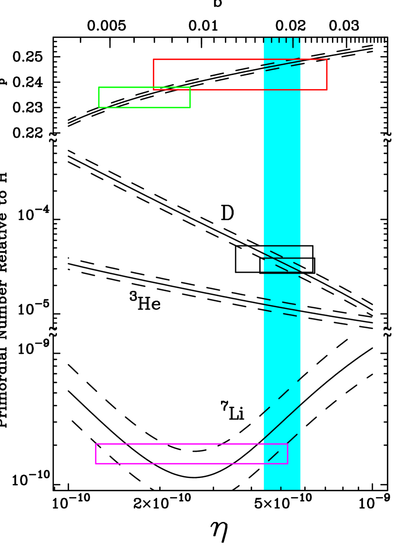
Figure 14: The predicted abundance ratios of the light elements from SBBN as a function of $\eta$ and $\Omega_{b}\,h^{2}$. ⁴He is shown as primordial mass fraction, Y_p. Boxes represent 95% confidence levels of recent observational determinations. The width of the boxes include 95% confidence levels in the SBBN calculations.

In Figure 14, we present the predicted abundances of the light elements relative to hydrogen in SBBN. The calculations assumed 3 species of light neutrinos and a neutron-half life of 887 s (Smith et al. (1993)). The dashed lines represent 95% confidence levels through Monte Carlo simulations of reaction rate and neutron lifetime uncertainties in the SBBN calculations (Sarkar (1996)).

The boxes represent the inferred primordial abundances through observations of D, ⁴He and ⁷Li. The two boxes which lie along the D abundance curve represent D/H measurement in QSO absorption systems. The larger box (larger uncertainties) represents the measurement presented here towards Q1009+2956, and the smaller represents the measurement by BT towards Q1937–1009. The combined result specifies 95% confidence levels in $\eta$, which is shown by the shaded region.

The constraint on $\eta$ given by the D/H measurement directly implies abundances for the other light elements. The implied abundances must fall in the shaded region in Fig. 14. For example, including SBBN uncertainties, D/H implies a primordial mass fraction of ⁴He,

$$Y_{p}=0.247\pm 0.001.$$ (6)

This range in D/H can be compared with two recent studies of ⁴He abundance measurements utilizing emission lines in metal-poor extragalactic H II regions. Our measurements of D/H are consistent with the inferred value of Y${}_{p}=0.243\pm 0.003$ found by Izotov et al. (1997) and shown by the larger box. Although D/H is not consistent with value found in another study by Olive et al. (1997), Y${}_{p}=0.234\pm 0.002$, shown in the smaller box. Unlike the two measurements constraining D/H, the determinations of Y_p are not mutually consistent.

The bottom curve in Fig. 13 shows the predicted SBBN yields of ⁷Li and the intersection with our confidence region from D/H. Due to large uncertainties in the reaction rates critical to ⁷Li, a given $\eta$ implies a large range of values for primordial ⁷Li. For example, our D/H measurements imply,

$$\rm{log({{{}^{7}Li}\over{H}})}_{p}=-9.5\pm 0.2,$$ (7)

which is higher than abundance inferred from the Spite “plateau” observed in warm metal-poor halo stars (Spite & Spite (1982), Spite et al. (1984), Rebolo et al. (1988), Thorburn (1994), Bonifacio & Molaro (1997)). The latest study by Bonifacio & Molaro (1997) use a better indicator of effective stellar temperatures, and infer a primordial abundance represented by the box in Fig. 14. Even though the observational errors are similar in magnitude to our D/H measurements (represented by the height of the boxes), the BBN uncertainties dominate the uncertainty when determining of $\eta$. The overlap of the box and shaded region shows the region of consistency between our values of D/H, and the abundance of ⁷Li given by Bonifacio & Molaro (1997). Although, primordial ⁷Li could be higher by as much as 0.6 dex, remain consistent with the D/H measurements, and accommodate non-standard models of lithium depletion (Vauclair & Charbonnel (1995), Pisonneault et al. (1992)).

We conclude that our D/H measurements 1) are likely the first measurements of a primordial abundance ratio of any element, 2) give the best determination of $\eta$ from SBBN and 3) are consistent with current observations of the other light elements.

5 IMPLICATIONS FOR IBBN

The measurements of low D/H in two separate high-redshift QSO absorption systems has immediate consequences for inhomogeneous models of Big Bang nucleosynthesis (IBBN). Jedamzik et al. (1993) first pointed out that observational constraints on the primordial value of D/H can directly test for and constrain the spatial variations of $\eta$ during the epoch of BBN. The amount of deuterium produced by BBN is very sensitive to both the average entropy density and the spatial variations in entropy. A generic feature of all IBBN models is that deuterium production is enhanced over standard homogeneous models (Jedamizk & Fuller (1994)). IBBN models which include either sub-horizon (Jedamzik et al. (1994)) or super-horizon (Jedamizk & Fuller (1995)) entropy fluctuations typically predict deuterium production which is 10 times greater than SBBN. Because deuterium production is so sensitive to $\eta$, high entropy regions are the dominant contributors to the cosmological deuterium abundance, even though these same regions contribute only a small fraction of the total mass.

We present two typical examples of IBBN in the context of the light element abundances of D, ⁴He, and ⁷Li. In the first example, we assume that the $\Omega_{b}$ is comparable to the value we found in the previous section, $\Omega_{b}\,h^{2}=0.02$. IBBN models can readily produce the inferred primordial abundance ratios of ⁴He and ⁷Li, but predict that the mass weighted cosmic average D/H $>10^{-4}$. Our two low measurements clearly rule this out if they represent the cosmic mean D/H. In the second example, we choose a much higher $\Omega_{b}$, so that the cosmic mean average in IBBN models can easily accommodate our measurements: $\Omega_{b}\,h^{2}=0.15$. All models of IBBN overproduce ⁴He and ⁷Li, with typical predictions of Y_p = 0.26 and ${}^{7}\rm{Li}/\rm{H}=10^{-9}$, which lie well beyond the upper limits inferred from extragalactic H II regions (Olive et al. (1997); Izotov et al. (1997)) and population II halo stars (Bonifacio & Molaro (1997)), respectively.

The simplest interpretation is that the low D/H measurements are consistent with the other light elements with predictions of homogeneous models of BBN. The assumption of SBBN is justified with a low primordial value of D/H. Following the conclusions of Jedamzik et al. (1994), we believe that our measurements of D/H not only provide observational constraints on $\eta$ and $\Omega_{b}$, but place limits on small scale entropy fluctuations during the epoch of BBN.

Date	Exposure (s)	XD Order	$\lambda_{min}$ (Å)	$\lambda_{max}$ (Å)
28 Dec 95	9000	1	3579.0	5529.0
28 Dec 95	7200	1	3579.0	5529.0
28 Dec 95	4800	2	3165.0	4330.0
09 Dec 96	7900	2	3135.0	4386.0
10 Dec 96	7800	2	3135.0	4386.0
10 Dec 96	8000	2	3135.0	4386.0

Table 1: HIRES Observations of Q1009+2956

Region	$\lambda_{min}$	$\lambda_{max}$	Pixels	Order	SNR
Ly$\alpha$	4254.50	4264.00	332	5	60
Ly$\beta$	3591.00	3596.60	231	3	25
Ly-6	3259.18	3262.20	155	3	13
Ly-12 – Ly-14	3208.00	3214.60	306	2	10
Ly-Limit	3199.40	3202.00	119	1	6

Table 2: Spectral Regions used in D/H Measurement

log N (cm-2 )	$b$(km s-1 )	$z$
12.65	9.6	1.63915
12.90	18.6	1.64226
13.53	75.3	1.64351
12.79	21.9	1.95511
13.31	19.7	1.95473
12.57	39.0	1.95722
13.14	28.8	2.50076
13.57	39.0	2.50456

Table 3: Extra H I Lines in D/H Models

Model	Com	D/H ($-2\sigma$)	D/H($\chi^{2}_{min}$)	D/H ($+2\sigma$)	$\chi^{2}_{min}$	n - $\nu$
1	3	$-4.44$	$-4.37$	$-4.28$	942.6	51
2	4	$-4.45$	$-4.37$	$-4.29$	906.1	55
3	5	$-4.43$	$-4.35$	$-4.26$	892.2	59
4	4	$-4.44$	$-4.34$	$-4.27$	903.5	55
5	4	$-4.52$	$-4.45$	$-4.39$	1076.1	41
6	4	$-4.56$	$-4.40$	$-4.28$	828.2	58

Table 4: D/H Absorption Models

Ion	Comp. 1		Comp. 2		Comp. 3
	$(z=2.50351)$		$(z=2.50357)$		$(z=2.50370)$
	Log N	b	Log N	b	Log N	b
H I	$15.79\pm 0.02$	$21.1\pm 8.1$	$16.93\pm 0.02$	$15.3\pm 3.0$	$17.07\pm 0.01$	$18.6\pm 5.7$
D I	11.39	$16.1\pm 7.9$	12.53	$11.6\pm 3.0$	12.67	$17.5\pm 5.5$
C I	$<12.2$	…	$<12.0$	…	$<12.0$	…
C II	$<12.4$	…	$12.30\pm 0.13$	$4.6\pm 2.3$	$12.18\pm 0.13$	$3.9\pm 2.4$
C III	$<12.3$	…	$13.31\pm 0.07$	$4.7\pm 0.8$	$13.44\pm 0.04$	$9.4\pm 2.4$
C IV	$<12.1$	…	$12.81\pm 0.02$	$5.4\pm 0.3$	$12.56\pm 0.03$	$5.6\pm 0.6$
N I	$<12.6$	…	$<12.3$	…	$<12.3$	…
N II	$<12.7$	…	$<12.4$	…	$<12.4$	…
N V	$<12.5$	…	$<12.4$	…	$<12.4$	…
O I	$<12.9$	…	$<13.0$	…	$<12.8$	…
Si II	$<11.8$	…	$<11.6$	…	$<11.5$	…
Si III	$<11.7$	…	$12.79\pm 0.05$	$4.6\pm 0.3$	$12.59\pm 0.02$	$4.5\pm 0.8$
Si IV	$<12.0$	…	$12.47\pm 0.02$	$4.0\pm 0.4$	$12.05\pm 0.03$	$3.9\pm 0.7$
Fe II	$<12.7$	…	$<12.4$	…	$<12.1$	…
Fe III	$<12.8$	…	$<12.5$	…	$<12.9$	…

Table 5: Column Densities of Metals

	Component 1	Component 2	Component 3
[C/H]	$<-2.8$	$-2.8$	$-3.0$
[N/H]	$<-0.4$	$<-1.7$	$<-1.8$
[Si/H]	$<-2.1$	$-2.4$	$-2.7$
[Fe/H]	$<0.8$	$<-0.9$	$<-0.7$
Log U	…	$-2.48$	$-2.58$
Log H I /H	…	$-2.97$	$-2.84$
Log $n_{\rm{H}}$ (cm-3)	…	$-2.30$	$-2.20$
L(kpc)	$>0.1$	5.0	3.0
Tb ($10^{4}$K)	$\approx 2.2$	1.2 $\pm$ 0.3	2.1 $\pm$ 0.5
Te ($10^{4}$K)	…	2.2	2.1
btur (km s-1 )	$\approx 8.5$	4.8 $\pm$ 0.8	1.9 $\pm$ 0.9

Table 6: Metallicity and Ionization State

Figure 1: Wide slit, flux-calibrated Lick spectra of Q1009+2956 ($z_{em}=2.63$, V=16.0). The figure contains three separate spectra of Q1009+2956 with different setups, and the flux calibration agrees between all three spectra. The 10$\sigma$ is shown as the solid line near 0.1. The Lyman limit of $z=2.504$ is the break in the flux near 3200 Å.

Figure 2: The Ly$\alpha$ forest of Q1009+2956 in the Lick spectrum (top panel) and the smoothed HIRES spectrum (bottom panel). The crosses in the top panel show the result of dividing the HIRES spectrum into the Lick spectrum, and represent the QSO continuum determined in the HIRES spectrum. The straight line is the fit to the crosses below 3750 Å(1030Årest), which we use to extrapolate the continuum below 3200 Å. The 10$\sigma$ is shown as the solid line near 0.2.

Figure 3: The Lick spectrum below the Lyman limit. The flux in shown in each pixel with 1$\sigma$ error bars. The solid line shows the model absorption profile with log[N(H I)_total] = 17.39 cm^-2 and additional absorption lines of H I with $z>2.0$. There is another Lyman limit system at $z=2.430$, with its break at $\lambda=3140$ Å. The dotted line corresponds to the 1$\sigma$ error in the measurement of N(H I)_total.

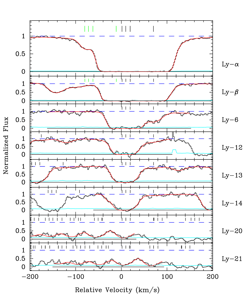
Figure 4: HIRES spectrum of Lyman series lines of the DHAS stacked in velocity space. Zero velocity corresponds to redshift $z=2.503571$. The histogram represents the normalized flux, each bin corresponds to a 2 km s^-1 pixel. The 1$\sigma$ error is gray solid line near zero. The smooth black line shows the best fit of Model 2. The ticks mark the velocity positions of individual components. This model has four main components, with three H I lines near 0 km s^-1 , three D I near $-82$ km s^-1 , and a fourth component of H I near 72 km s^-1 . The solid black line at zero flux shows the regions about each Lyman line used in the fitting procedure.

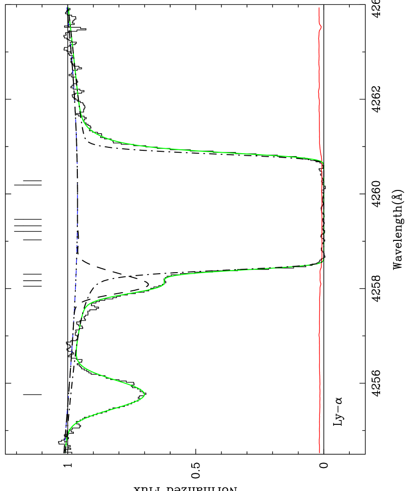
Figure 6a: The Ly$\alpha$ absorption feature at $z=2.504$. The histogram shows the same spectrum as in Fig. 4. The spectrum has been normalized to the initial continuum estimate, which is the solid black line at unity. The best fit continuum is the 5th order Legendre polynomial which drops below un ity. The profile fits of D and H are shown as dashed and dot-dashed lines, respectively. The tallest tick marks show the line centers of the three main H components in Model 2. The corresponding D components are the three tick marks to the left, and the additional hydrogen component is the lone tick mark to the right. The grey line represents the total absorption model fit.

Figure 6b: HIRES Spectrum of the Ly$\beta$ region of the DHAS. The continuum is a 3rd order Legendre polynomial. Extra H I absorption can be seen left of the position of D-Ly$\beta$ . The gray line represents the same model as in Fig 6a.

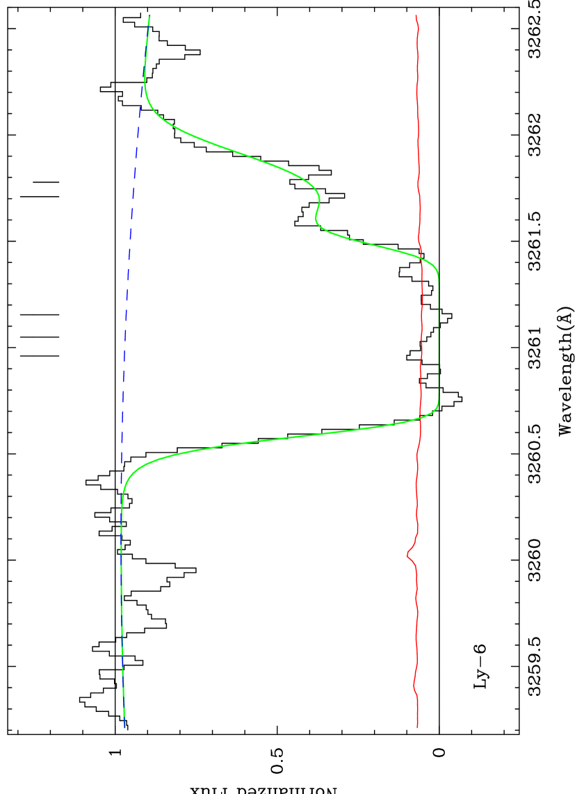
Figure 6c: HIRES Spectrum of the Ly-6 region of the DHAS. The continuum is a 3rd order Legendre polynomial. The gray line represents the same model as in Fig 6a.

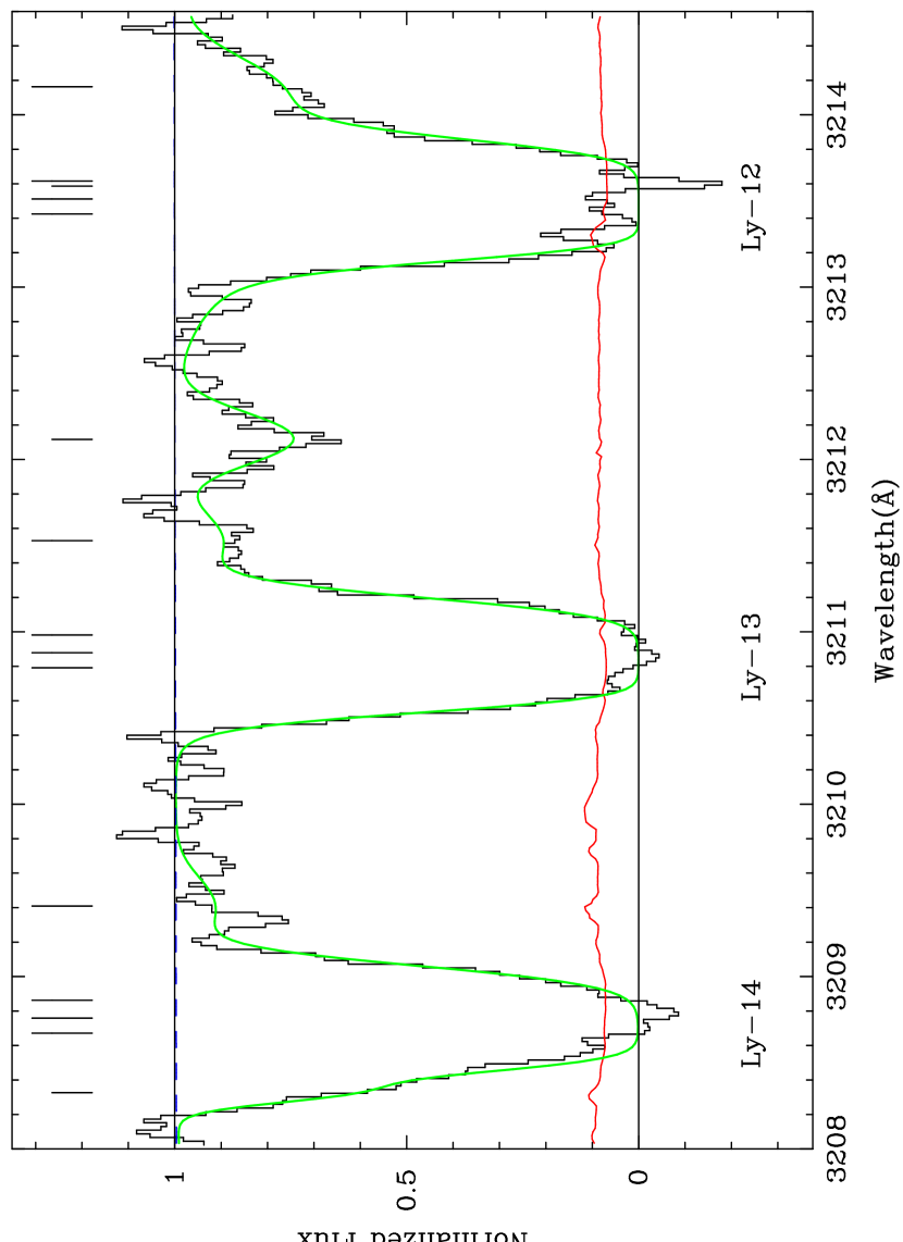
Figure 6d: HIRES Spectrum of the region containing Ly-12 to Ly-14 of the DHAS. The continuum is a 2nd order Legendre polynomial. The gray line represents the same model as in Fig 6a.

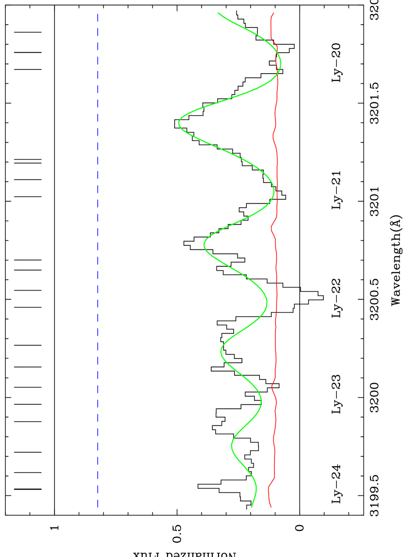
Figure 6e: HIRES Spectrum of the region containing Ly-20 to Ly-24 of the DHAS. The continu um is a 1st order Legendre polynomial. The gray line represents the same model as in Fig 6a.

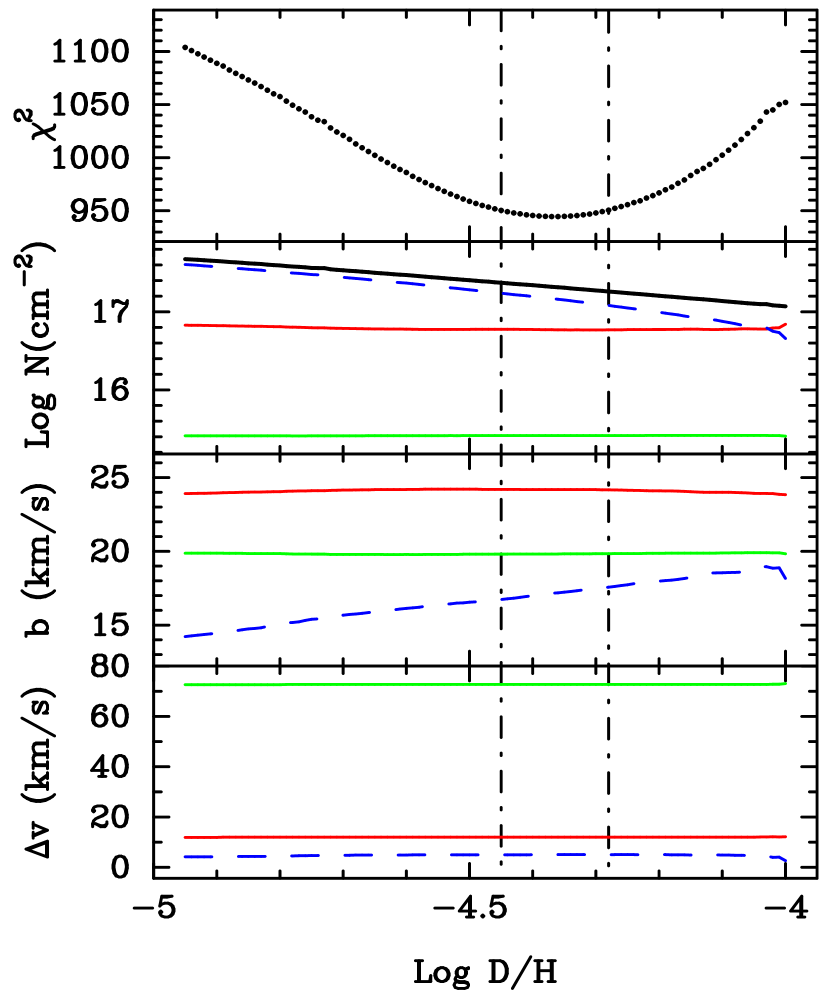
Figure 7a: Results of the fitting procedure for Model 1. The top panels show the $\chi^{2}_{min}$ functions vs. D/H, and the vertical dot-dashed lines encompass the minima and represent 95% confidence levels in each model. The second panel shows the column densities of main H I components, with each component’s value represented with a different line style. The thick solid line shows N(H I)_total (the sum of column densities) as a function of D/H. The third panel shows the velocity dispersions of the hydrogen components, and the fourth shows the the velocity position relative to $z=2.503571$.

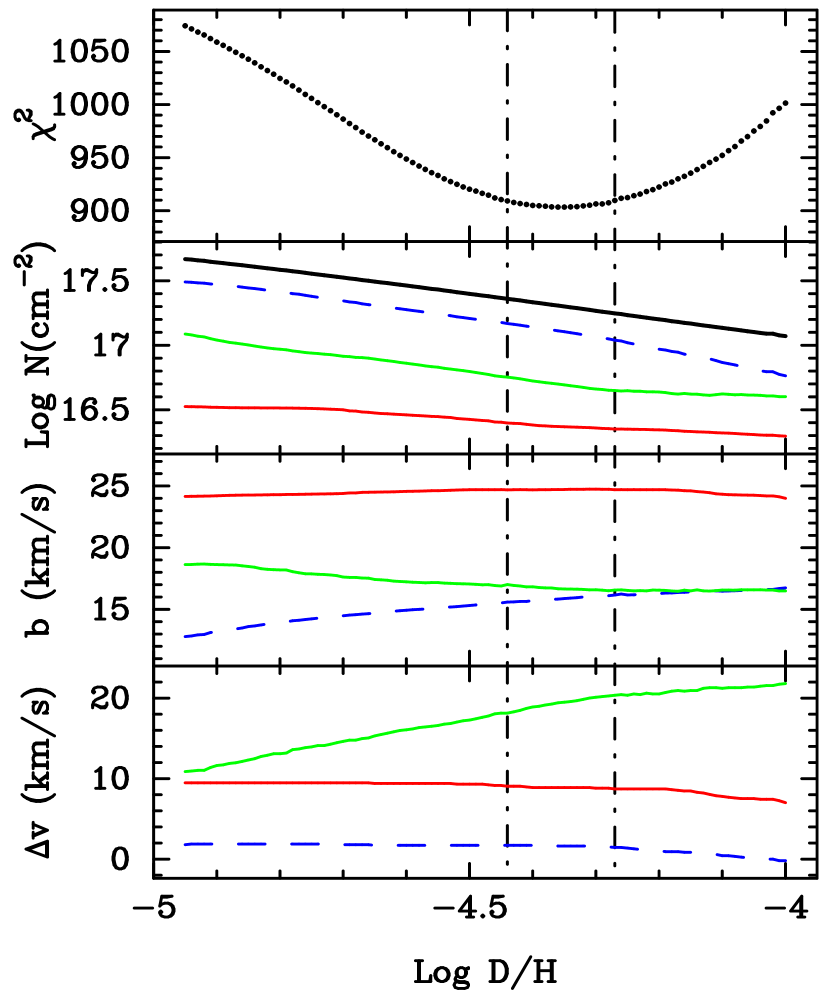
Figure 7b: Results of Model 2

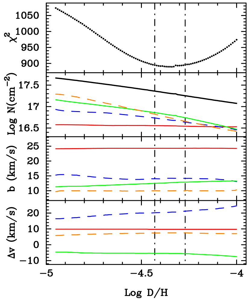
Figure 7c: Results of Model 3

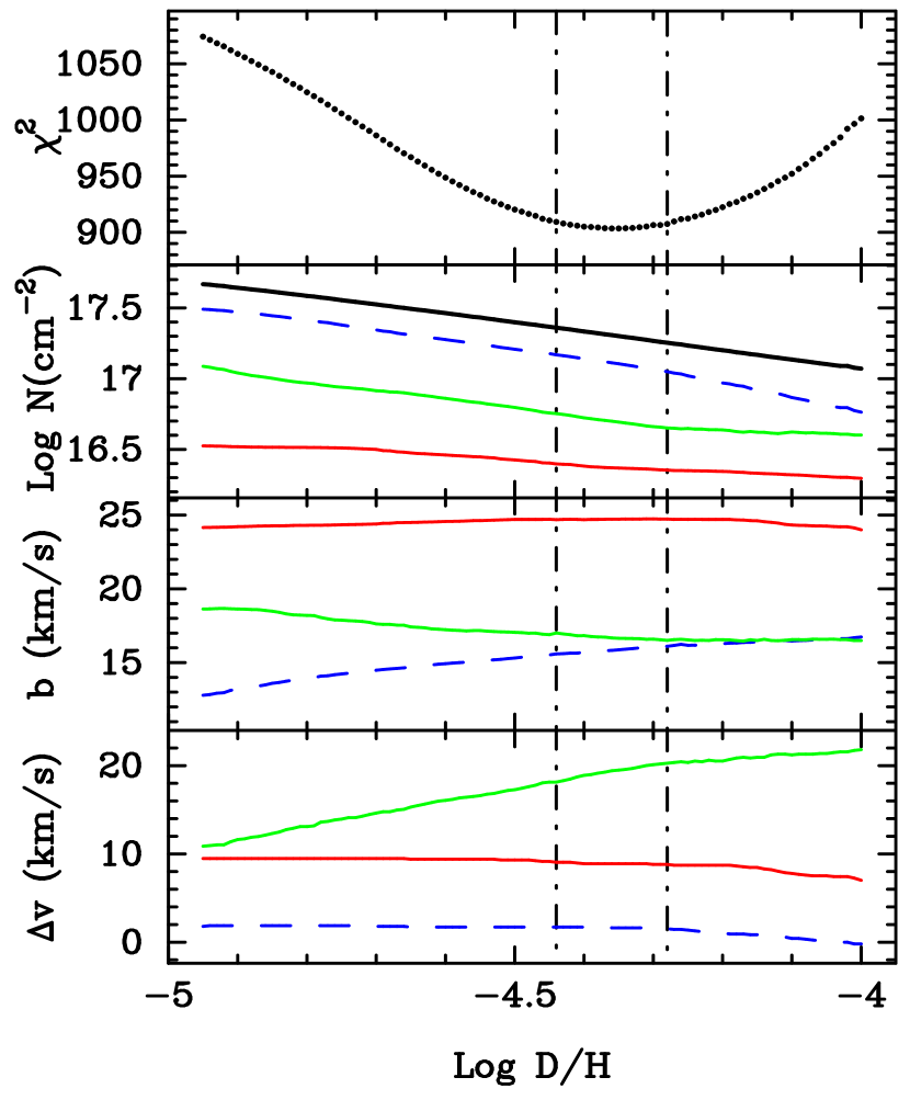
Figure 7d: Results of Model 4

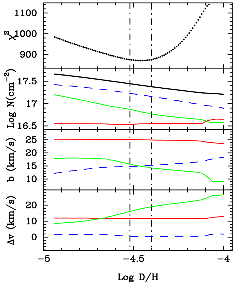
Figure 7e: Results of Model 5

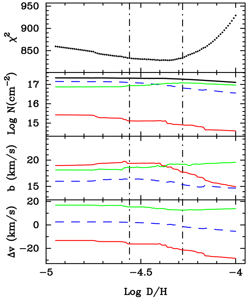
Figure 7f: Results of Model 6

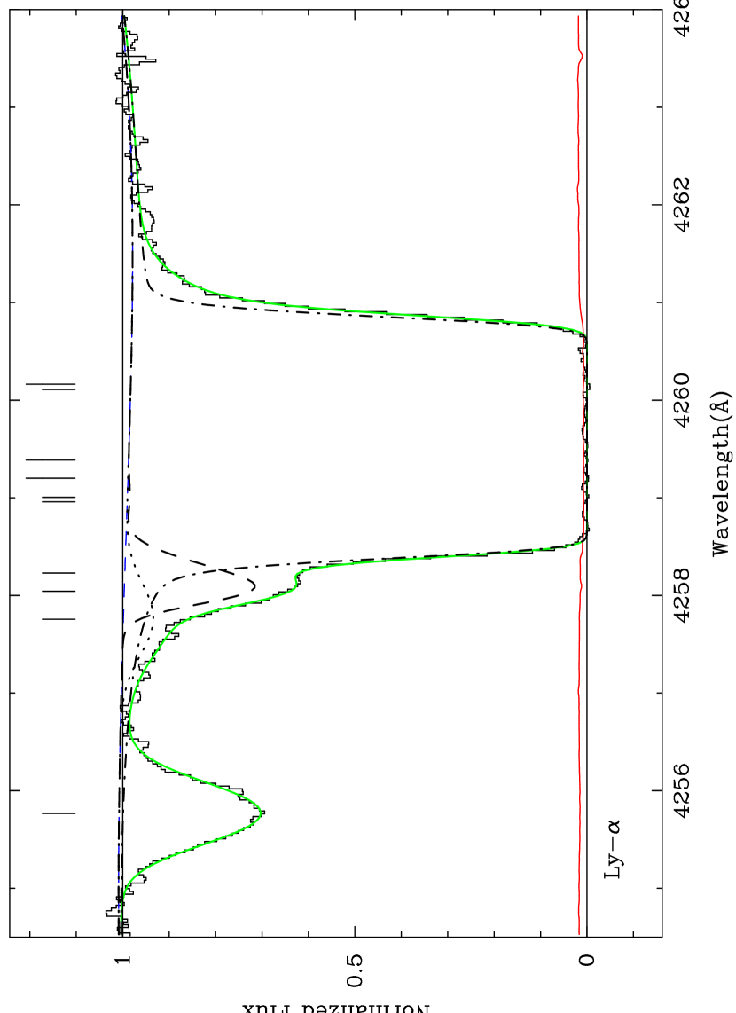
Figure 8a: Same as Fig. 6a, but shows the best fits for Model 6 (with contamination). The dotted line shows the profile of the H I contamination near the deuterium feature.

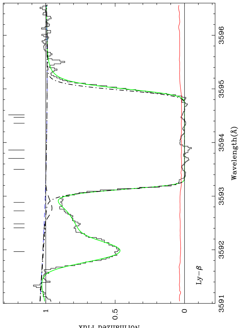
Figure 8b: Same as Fig. 8a, but for Ly$\beta$ .

Figure 9: Summary of 95% confidence intervals in the six models

Figure 11: Likelihood of D/H with contamination. The top panel shows the $\chi^{2}$ function from Fig. 9, the middle panel shows the probability of a random Ly$\alpha$ line with a minimum column density falling near deuterium, and the bottom panel shows the combined likelihood.

Figure 12: Zero velocity corresponds to redshift $z=2.503571$ to match Fig. 4. The dotted lines correspond to absorption components at the velocity positions given by the best fit to the Lyman series in Model 6.

Figure 13: Total $\chi^{2}$ of Q1937–1009 and Q1009+2956

References

- Adams (1976) Adams, T. F. 1976, A&A, 50, 461
- Audouze & Tinsley (1974) Audouze, J., & Tinsley, B. 1974, ApJ, 192, 487
- Balser et al. (1994) Balser, D. S., Bania, T. M., Brockway, C. J., Rood, R. T., & Wilson, T. L. 1994, ApJ, 430, 667
- Balser et al. (1997) Balser, D. S., Bania, T. M., Rood, R. T., & Wilson, T. L. 1997, ApJ, 483, 320
- Bonifacio & Molaro (1997) Bonifacio, P., & Molaro, P. 1997, MNRAS, 285, 847
- Burles & Tytler (1996) Burles, S., & Tytler, D. 1996, ApJ, 460, 584
- Burles & Tytler (1996) Burles, S., & Tytler, D. 1996, astro-ph 9603070
- (8) Burles, S., & Tytler, D. 1997, AJ, in press
- (9) Burles, S., & Tytler, D. 1997, submitted to ApJ (BT)
- Burles (1997) Burles, S. 1997, in preparation
- Cardall & Fuller (1996) Cardall, C. Y. & Fuller, G. M. 1996, ApJ, 472, 435
- Carlberg et al. (1997) Carlberg, R. G., Morris, S. L., Yee, H. K. C., Ellingson, E., Abraham, R., Lin, H., Schade, D., Gravel, P., Pritchet, C. J., Smecker-Hane, T., Hartwick, F. D. A., Hesser, J. E., Hutchings, J. B., & Oke, J. B. 1997, submitted to ApJ Letters
- Carswell et al. (1994) Carswell, R. F., Rauch, M., Weymann, R. J., Cooke, A. J. & Webb, J. K. 1994, MNRAS, 268, L1
- Carswell et al. (1996) Carswell, R. F., Webb, J. K., Lanzetta, K. M., Baldwin, J. A., Cooke, A. J., Williger, G. M., Rauch, M., Irwin, M. J., Robertson, J. G., & Shaver, P. A. 1996, MNRAS, 278, 506
- Chengular et al. (1997) Chengalur, J. N., Braun, R. & Burton, W. B. 1997, A&A, 318, L35
- Clayton (1985) Clayton, D. D. 1985, ApJ, 290, 428
- Copi et al. (1995) Copi, C.J., Schramm, D.N. & Turner, M.S. 1995, Science, 267, 192
- Edmunds (1994) Edmunds, M.G. 1994, MNRAS, 270, L37
- Epstein et al. (1976) Epstein, R. I., Lattimer, J. M., & Schramm, D. N. 1976, Nature, 268, 198
- Ferland (1993) Ferland, G. 1993, Univ. Kentucky Dept. Physics and Astron. Internal Rept.
- Fields (1996) Fields, B. 1996, ApJ, 456, 478
- Fixsen et al. (1996) Fixsen, D. J., Cheng, E. S., Gales, J. M., Mather, J. C., Shafer, R. A., & Wright, E. L. 1996, ApJ, 473, 576
- Fuller & Shi (1997) Fuller, G. M., & Shi, X. 1997, ApJ, in press
- Fuller & Cardall (1996) Fuller, G. M., & Cardall, C. Y. 1996, Nucl. Phys. Proc. Suppl. B, 51, 71
- Galli et al. (1995) Galli, D., Palla, F., Ferrini, F. & Penco, U. 1995, ApJ, 443, 536
- Geiss (1993) Geiss, J. 1993, in ”Origin and Evolution of the Elements”, eds. N. Prantzos, E. Vangioni-Flam, & M. Casse (Cambridge University Press: Cambridge), 89
- Giallongo et al. (1997) Giallongo, E., Fontana, A., & Madau, P. 1997, submitted to MNRAS
- Haardt & Madau (1997) Haardt, F. & Madau, P. 1997, ApJ, 461, 20
- Hata et al. (1997) Hata, N., Steigman, G., Bludman, S., & Langacker, P. 1997, Phys. Rev. D, 55, 540
- Hu & White (1996) Hu, W., & White, M. 1996, ApJ, 471, 30
- Izotov et al. (1997) Izotov, Y. I., Thuan, T. X., & Lipovetsky, V. A. 1997, ApJS, 108, 1
- Jedamzik (1993) Jedamzik, K. 1993, Ph.D. Thesis, University of California, San Diego
- Jedamizk & Fuller (1994) Jedamzik, K., & Fuller, G. M. 1994, ApJ, 423, 33
- Jedamzik et al. (1994) Jedamzik, K., Fuller, G. M., & Mathews, G. 1994, ApJ, 423, 50
- Jedamizk & Fuller (1995) Jedamzik, K., & Fuller, G. M. 1995, ApJ, 452, 33
- Jedamzik & Fuller (1997) Jedamzik, K. & Fuller, G. M. 1997, ApJ, 483, 560
- Kawano (1992) Kawano, L. 1992, preprint
- Kirkman & Tytler (1997) Kirkman, D. & Tytler, D. 1997, ApJ, 484, 848
- Krauss & Kernan (1995) Krauss, L. M., Kernan, P. J. 1995, Phys. Lett. B, 347, 347
- Lemoine et al. (1996) Lemoine, M., Vidal-Madjar, A., Bertin, P., Ferlet, R., Gry, C., & Lallement, R. 1996, A&A, 308, 601
- Levshakov et al. (1996) Levshakov, S. A., & Kegel, W. H. 1996, MNRAS, 278, 497
- Lu et al. (1997) Lu, L., Sargent, W. L. W., & Barlow, T. A. 1997, submitted to ApJ
- Olive & Steigman (1995) Olive, K. A. & Steigman, G. 1995, ApJS, 97, 49
- Olive et al. (1997) Olive, K. A., Skillman, E. D., & Steigman, G. 1997, ApJ, 483, 788
- Persic & Salucci (1992) Persic, M. & Salucci, P. 1992, MNRAS, 258, 14
- Piskunov et al. (1997) Piskunov, N., Wood, B. E., Linsky, J. L., Dempsey, R. C., Ayres, T. R. 1997 ApJ, 474, 315
- Pisonneault et al. (1992) Pisonneault, M. H., Deliyannis, C. P., Demarque, P. 1992, ApJS, 78, 179
- Prantzos (1996) Prantzos, N. 1996, A&A, 310, 106
- Press et al. (1992) Press, W. H., Teukolsky, S. A., Vetterling, W. T., & Flannery, B. P. 1992, Numerical Recipes in C, the Art of Scientific Computing, 2nd ed. (Cambridge, UK: Cambridge University Press)
- Rauch et al. (1997) Rauch, M., Miralda-Escude, J., Sargent, W. L. W., Barlow, T. A., Weinberg, D. H., Hernquist, L., Katz, N., Cen, R., & Ostriker, J. P. 1997, submitted to ApJ
- Rebolo et al. (1988) Rebolo, R., Beckman, J. E., & Molaro, P. 1988, A&A, 192, 192
- Reeves et al. (1972) Reeves, H., Audouze, J., Fowler, W. A., & Schramm, D. N. 1973 ApJ, 179, 909
- Reimers et al. (1995) Reimers, D., Rodriguez-Pascual, P., Hagen, H. J., & Wisotzki, L. 1995, A&A, 293, L21
- Reimers et al. (1997) Reimers, D., Koehler, S., Wisotzki, L., Groote, D., Rodriguez-Pascual, P., Wamsteker, W. 1997, submitted to A&A, astro-ph/9707173
- (55) Rugers, M., & Hogan, C. 1996, ApJ, 459, L1
- (56) Rugers, M., & Hogan, C. 1996, AJ, 111, 2135
- Sarkar (1996) Sarkar, S. 1996, Rep. Prog. Phys., 59, 1493
- Scully et al. (1997) Scully, S., Casse, M., Olive, K. A., & Vangioni-Flam, E. 1997, ApJ, 476, 521
- Schramm & Turner (1997) Schramm, D. N. & Turner, M. S. 1997, submitted to Rev. Mod. Phys.
- Smith et al. (1993) Smith , M. S., Kawano, L. H. & Malaney, R. A. 1993, ApJS, 85, 219
- Songaila et al. (1994) Songaila. A., Cowie, L. L., Hogan C. J. & Rugers, M. 1994, Nature, 368, 599
- Spite & Spite (1982) Spite, F., & Spite, M. 1982, A&A, 115, 357
- Spite et al. (1984) Spite, M., Maillard, J. P., & Spite, F. 1984, A&A, 141, 56
- Spitzer (1978) Spitzer, L., Jr. 1978, Physical processes in the interstellar medium (New York, NY: Wiley)
- Steigman & Tosi (1992) Steigman, G. & Tosi, M. 1992, ApJ, 401, 150
- Steigman & Tosi (1995) Steigman, G. & Tosi, M. 1995, ApJ, 453, 173
- Thorburn (1994) Thorburn, J. A. 1994, ApJ, 421, 318
- Tytler (1982) Tytler, D. 1982, Nature, 298, 427
- Tytler et al. (1996) Tytler, D., Fan, X-M., & Burles, S. 1996, Nature, 381, 207 (TFB)
- Tytler & Burles (1997) Tytler, D., & Burles, S. 1997, in ”Origin of Matter and Evolution of Galaxies”, eds. T. Kajino, Y. Yoshii & S. Kubono (World Scientific Publ. Co.: Singapore), 37
- (71) Tytler, D., Burles, S., & Kirkman, D. 1996, submitted to ApJ
- Vangioni-Flam et al. (1994) Vangioni-Flam, E., Olive, K. A., Prantzos, N. 1994, ApJ, 427, 418
- Vauclair & Charbonnel (1995) Vauclair, S., & Charbonnel, C. 1995, A&A, 295, 715
- Wagoner et al. (1967) Wagoner, R. V., Fowler, W. A., & Hoyle, F. 1967, ApJ, 148, 3
- Walker et al. (1991) Walker, T. P., Steigman, G., Schramm, D. N., Olive, K. A. & Kang, H. S. 1991 ApJ, 376, 51
- Wampler et al. (1996) Wampler, E.J., Williger, G.M., Baldwin, J.A., Carswell, R.F., Hazard, C. & Mcmahon, R.G. 1996, A&A, 316, 33
- Webb et al. (1997) Webb, J. K., Carswell, R. F., Lanzetta, K. M., Ferlet, R., Lemoine, M., Vidal-Madjar, A., & Bowen, D. V. 1997, Nature, 388, 250
- Weinberg et al. (1997) Weinberg, D. H., Miralda-Escude, J., Hernquist, L., & Katz, N. 1997, submitted to ApJ
- Zhang et al. (1997) Zhang, Y., Meiksin, A., Anninos, P., Norman, M. L. 1997, ApJ, in press