The K band Hubble diagram for brightest cluster galaxies in X-ray clusters

Abstract

This paper concerns the K band Hubble diagram for the brightest cluster galaxies (BCGs) in a sample of X-ray clusters covering the redshift range $0.05<z<0.8$. We show that BCGs in clusters of high X-ray luminosity are excellent standard candles: the intrinsic dispersion in the raw K band absolute magnitudes of BCGs in clusters with $L_{\rm X}>2.3\times 10^{44}$ erg s^-1 (in the 0.3 - 3.5 keV band) is no more than 0.22 mag, and is not significantly reduced by correcting for the BCG structure parameter, $\alpha$, or for X-ray luminosity. This is the smallest scatter in the absolute magnitudes of any single class of galaxy and demonstrates the homogeneity of BCGs in high-$L_{\rm X}$ clusters. By contrast, we find that the brightest members of low-$L_{\rm X}$ systems display a wider dispersion ($\sim 0.5$ mag) in absolute magnitude than commonly seen in previous studies, which arises from the inclusion, in X-ray flux-limited samples, of poor clusters and groups which are usually omitted from low redshift studies of BCGs in optically rich clusters.

Spectral synthesis models reveal the insensitivity of K band light to galaxy evolution, and this insensitivity, coupled with the tightness of its Hubble relation, and the lack of evidence of significant growth by merging (shown by the absence of a correlation between BCG structure parameter, $\alpha$, and redshift), makes our sample of BCGs in high-$L_{\rm X}$ clusters ideal for estimating the cosmological parameters $\Omega_{\rm M}$ and $\Omega_{\Lambda}$, free from many of the problems that have bedevilled previous attempts using BCGs. The BCGs in our high-$L_{\rm X}$ clusters yield a value of $\Omega_{\rm M}=0.28\pm 0.24$ if the cosmological constant $\Lambda=0$. For a flat Universe we find $\Omega_{\rm M}=0.55^{+0.14}_{-0.15}$ with a 95 per cent confidence upper limit to the cosmological constant corresponding to $\Omega_{\Lambda}<0.73$. These results are discussed in the context of other methods used to constrain the density of the Universe, such as Type Ia supernovae.

1 INTRODUCTION

The Hubble (redshift–magnitude) diagram for brightest cluster galaxies (BCGs) is a classic cosmological tool (recently reviewed by Sandage 1995). Sandage and collaborators (e.g. Sandage 1972a,b; Sandage & Hardy 1973; Sandage, Kristian & Westphal 1976) used the Hubble diagram for BCGs to verify Hubble’s linear redshift–distance law out to a distance one hundred times greater than that probed by the initial bright galaxy sample of Hubble (1929), and attempted to measure the deceleration parameter from its deviation from the linear Hubble law. More recently, the BCG redshift–magnitude relation has appeared in studies of the formation and evolution of elliptical galaxies (Aragón–Salamanca et al. 1993) and of large-scale bulk flows in the Universe (Lauer & Postman 1994; Postman & Lauer 1995; Hudson & Ebeling 1997).

Underlying all this work is the fact that BCGs appear to be good standard candles after correction for systematic effects and the dependence of absolute magnitude on galaxy structure and environment, with their aperture luminosities at low redshift showing a dispersion of only $\sim 0.3$ mag (Sandage 1988). This small dispersion is all the more remarkable since BCGs do not appear to be a particularly homogeneous class of objects at first sight: some exhibit the large, extended envelopes that make them cD galaxies; many (up to half according to Hoessel & Schneider 1985) have multiple nuclei; and their immediate local environments vary from relative isolation in the cluster core to interaction and merging, in the case of dumbbell galaxies. BCGs tend to dominate their host clusters visually, but little is known of their place in the formation and evolution of the clusters, or of their own origins.

Answers to some of these questions may result from extending the Hubble diagram for BCGs to higher redshifts, but there are several problems with that. Firstly, as one moves to higher redshifts, optical wavebands become increasingly sensitive to the effects of star formation, and K-corrections become large and uncertain. This problem may be circumvented, as discussed in detail below, by working in the K band, which continues principally to sample the mature stellar population out to high redshifts: the K band Hubble diagram for a small sample of BCGs was presented by Aragón–Salamanca et al. (1993).

A more serious problem is that of cluster selection. In the past, cluster samples have been selected from optical surveys, on the basis of identifying enhancements in the surface density of galaxies above a fluctuating background. Such a procedure suffers from the well-known projection effects caused by chance alignments of galaxies along the line-of-sight (van Haarlem, Frenk & White 1997, and references therein). This contamination will be more severe at fainter magnitudes, thus strongly discouraging the use of this method for detecting high-redshift clusters. A solution to this problem is provided by X-ray cluster selection. Most bona fide clusters contain hot gas in their cores, emitting a copious flux of X-rays and making them visible to large distances. The intensity of the thermal bremsstrahlung X-ray emission from a cluster is directly related to the depth of its gravitational potential well, unlike its optical galaxy richness, while the compactness of the X-ray-emitting region, compared to the extent of the galaxy distribution, also means that projection effects are minimal in comparison to those arising in optical cluster selection (Romer et al. 1994; van Haarlem et al. 1997).

These concerns motivated the current study, the long-term goal of which is to investigate the formation and evolution of BCGs in host clusters with known X-ray luminosities, by studying their physical properties over a wide span of cosmological time. In this paper we concentrate on extending the infrared Hubble diagram for BCGs to higher redshifts than studied before using K band images of a large sample of BCGs in X-ray clusters with $z\la 0.8$. The plan of the remainder of this paper is as follows. In Section 2 we briefly describe our cluster sample, the observations made and their reduction, leading to the presentation of the uncorrected $K-z$ diagram for our sample in Section 3, followed by a discussion of K-correction models for our BCGs in Section 4. We consider the physical properties of the BCGs and their host clusters in Section 5 and look for correlations between them in Section 6. These correlations are used to produce a corrected Hubble diagram in Section 7, which is used to derive constraints on the cosmological parameters $\Omega_{\rm M}$ and $\Omega_{\Lambda}$ in Section 8. In Section 9 we discuss the results of this paper and present the conclusions we draw from them. An Appendix tabulates some statistical results omitted from the main body of the text.

2 THE DATA

2.1 The X-ray Cluster Sample

The X-ray clusters for this work were chosen principally from the Einstein Medium Sensitivity Survey (Gioia et al. 1990, Stocke et al. 1991, hereafter EMSS) catalogue of 104 X-ray selected clusters (Gioia & Luppino 1994), but supplemented by two clusters from the ROSAT All–Sky Survey (Voges 1992, Trümper 1993). Fig. 1 shows the X-ray luminosities listed in Gioia & Luppino (1994) for all the EMSS clusters, as a function of redshift, compared with the sample studied here: the X-ray luminosities were calculated assuming that $\Omega_{\rm M}=1$, $\Omega_{\Lambda}=0$ and the Hubble constant is $H_{0}=50$ km s^-1 Mpc^-1. No attempt was made to observe a statistically complete subsample of EMSS clusters, although it is clear from Fig. 1 that those selected are broadly representative of the range of X-ray luminosities for clusters within the parent survey: a two–sided Kolmogorov–Smirnov (K-S) test yields a probability of 0.26 that the cumulative X-ray luminosity distributions of the EMSS clusters imaged and not imaged would differ by more than observed if both subsamples were drawn from the same parent distribution. The corresponding K-S test on the redshift distributions of EMSS cluster subsamples imaged and not imaged yields a probability of only 0.04, reflecting the fact that we preferentially selected EMSS clusters at higher redshifts, where the luminosity distance varies appreciably with cosmology and, thus, constraints on $\Omega_{\rm M}$ and $\Omega_{\Lambda}$ may be derived from the BCG Hubble diagram.

Figure 1: The luminosities of the EMSS clusters (in the 0.3–3.5 keV passband) against redshift. The filled circles are the clusters imaged at K and discussed in this paper, while the empty circles are the rest of the EMSS cluster sample of Gioia & Luppino (1994). The two triangles are the ROSAT clusters. Note that there is no single, sharp flux limit to the EMSS survey – cluster detections were based on pointed observations whose limiting sensitivity ranges from $5\times 10^{-14}$ erg cm^-2 s^-1 to $3\times 10^{-12}$ erg cm^-2 s^-1.

2.2 Observations

Observations were made on 8-10 November 1994 and 20-22 April 1995 using the IRCAM3 infrared camera on the 3.8m United Kingdom Infrared Telescope (UKIRT): IRCAM3 contains a $256\times 256$ InSb array, with a pixel size of 0.286 arcsec. Two observing procedures were followed. For distant clusters, a series of 100s (10 $\times$ 10s co-added) exposures were taken, with the galaxy offset in a five-point jitter pattern within the initial field of view of the chip. For nearby clusters, where the BCG covered too large an area of the chip to allow accurate sky level determination by this method, sky exposures were obtained after each galaxy exposure, allowing the jitter pattern for the sky frames (four-, or eight-point) to be built-up simultaneously with that of the jitter pattern for the galaxy frames (five-, or nine-point). Typical total on-source integration times used were $\sim 1000$s for $z\la 0.2$, 1500-3000s for $0.2\la z\la 0.4$ and 4500s above $z=0.5$. Dark frames were taken regularly throughout the nights, as were standard star observations, using sources from the UKIRT Faint Standards list (Casali & Hawarden 1992).

2.3 Data Reduction

The data were reduced using standard iraf routines and the following procedure. Appropriate dark frames were subtracted from each galaxy or sky image, and the resulting frames were multiplied by a mask, flagging known bad pixels in the array to be ignored subsequently, before normalising the frames to unit median: we found the median to be a more stable measure of the sky level than the mode. Flat-field frames were constructed, by median filtering the galaxy frames (for distant clusters) or sky frames (for nearby clusters), and these flat frames were normalised to unit median. The galaxy frames were then divided by the appropriate flat field frame and final mosaic images produced by cross-correlating the individual flat-fielded galaxy frames to determine their relative offsets. A similar procedure was used to reduce the standard star frames.

A total of 52 BCGs were observed. Two of these, (those in MS1401.9+0437 and MS1520.1+3002), did not yield photometric quality data and were dropped from our sample, as were two others (MS1209.0+3917 and MS1333.3+1725) which have dubious redshift identifications in Gioia & Luppino (1994). A fifth BCG, in MS0440.5+0204, was subsequently omitted, because it is close to a bright star, which falls within our chosen photometric aperture. This left us with a sample of 47 BCGs: note that Stocke et al. (1991) and Gioia & Luppino (1994) suggest that the two EMSS sources MS2215.7-0404 and MS2216.0-0401 may be part of the extended X-ray emission from a single cluster, but we have treated them as two distinct objects. We assume cosmological matter and vacuum energy densities of $\Omega_{\rm M}=1$ and $\Omega_{\Lambda}=0$, respectively, and $h=0.5$ (where $H_{0}=100h\,{\rm kms}^{-1}{\rm Mpc}^{-1}$ is the Hubble constant) throughout this paper, unless stated otherwise.

Figure 2: The raw $K-z$ diagram. The filled circles show the apparent K band magnitudes of the 47 BCGs in our X-ray sample, while the empty circles are the BCGs from the optical sample of Aragón-Salamanca et al. (1993), excluding the one BCG in common between the two samples. The magnitudes are corrected for Galactic extinction, but have not been K-corrected.

3 THE RAW $\mn@boldsymbol{K}$–$\mn@boldsymbol{z}$ DIAGRAM

We obtained K band aperture magnitudes for our BCGs using the iraf package apphot, with a fixed metric aperture of diameter 50 kpc: in the few cases, where there were two similarly bright galaxies in the cluster, the BCG was taken to be the brighter of the two as judged by this magnitude. Airmass corrections were made using the standard median Mauna Kea K band extinction value of 0.088 mag/airmass.

The choice of aperture was made on the basis of two considerations. Firstly, it allows direct comparison with the results of Aragón-Salamanca et al. (1993) who studied BCGs in nineteen optically-selected clusters. Secondly, as discussed in Section 5.1, we require a sufficiently large metric aperture to allow accurate estimation of the BCG structure parameter, $\alpha$, for our more distant clusters, given the seeing conditions obtaining during our runs.

From comparing frames of the same object taken at different times on the same night, on different nights of the same run and between the two runs, we obtain formal statistical errors of 0.04 to 0.07 mags on our 50 kpc magnitudes, except for 11 BCGs observed on one particular night for which greater uncertainty in our photometric calibration produced uncertainties of 0.1 mags. For the one object (MS0015.9+1609 $\equiv$ Cl0016+16) we have in common with Aragón-Salamanca et al. (1993) they measure an aperture magnitude that agrees with ours to well within these estimated errors (15.56 mag compared to our 15.58 mag). In addition to these statistical errors, there are likely to be systematic errors resulting, for example, from contamination from other cluster galaxies falling within the photometric aperture: we make no attempt to estimate these (necessarily very uncertain) corrections. The aperture magnitude data set is given in Table 2 and the resultant raw $K-z$ diagram is shown in Fig. 2. It is clear from Fig. 2 that there is a large scatter in the raw $K-z$ diagram for the BCGs in our X-ray cluster sample, and that most of the scatter comes from the lower-$z$ half of the sample: before expressing that scatter in terms of the rms dispersion in the absolute magnitudes of the galaxies, and investigating its origin, we must discuss how to K–correct the galaxy magnitudes, which we do in the next Section.

4 Interpreting the BCG K band magnitudes

There is a consensus developing that cluster ellipticals are old, for example: Charlot & Silk (1994) model the evolution of spectral indicators of E/S0 galaxies in low-redshift ($z<0.4$) clusters, and suggest that a couple of per cent at most of their stars have been made in the past 2.5 Gyr; Bender, Ziegler & Bruzual (1996) use Mg${}_{b}-\sigma$ data for 16 cluster ellipticals in three clusters at $z\simeq 0.37$ to show that the majority of their stars must have formed at $z>2$, and that the most luminous galaxies may have formed at $z>4$; and Ellis et al. (1997) use rest–frame UV–optical photometry of ellipticals in $z\sim 0.5$ clusters obtained with the Hubble Space Telescope to show that the bulk of the star formation in the ellipticals in dense clusters was completed before $z\sim 3$ in conventional cosmologies. If we assume that the same goes for our BCGs as for cluster ellipticals in general, then our photometric data are easy to interpret, since, by choosing the K band, we are primarily sampling the passively evolving mature stellar population over our full redshift range, and the resultant K–correction will be insensitive to the exact age of the galaxy: we take the K–correction, $K(z)$, as encompassing the bandwidth, band–shifting and evolution terms (e.g. Sandage 1995), defining it so that the absolute magnitude, $M$, of a galaxy observed to have an apparent magnitude $m$ at redshift $z$ is given by $M=m+5-5\log_{10}(d_{\rm L})-K(z)$, where $d_{\rm L}(z,\Omega_{\rm M},\Omega_{\Lambda},H_{0})$ is the luminosity distance (in pc), and where we have neglected the effect of Galactic extinction.

In the light of these results, we take as our default K–correction model that resulting from a Bruzual & Charlot GISSEL (Bruzual & Charlot 1993) model (1995 version: see Charlot, Worthey & Bressan 1996) in which our BCGs form in a 1 Gyr burst (with a Salpeter 1955 IMF, over the range $0.1\leq M/M_{\odot}\leq 125$) at a redshift $z_{\rm f}=3$, in a Universe with $\Omega_{\rm M}=1$, $\Omega_{\Lambda}=0$, and $h=0.5$. This can be approximated to better than 0.02 mag over the range $0\leq z\leq 1$ by a fifth-order polynomial in $z$, given by

$$K(z)=-2.476z-0.5809z^{2}+14.04z^{3}-21.10z^{4}+9.147z^{5}.$$ (1)

This is computed by approximating the K band filter by a top-hat between 2.0 and 2.45 $\mu$m: the computed K-correction changes by $\la 0.02$ mag over $0\leq z\leq 1$ if instead we fit the UKIRT K band filter (S.K. Leggett, private communication) with a ninth-order polynomial, which accurately follows variations in its transmission from 1.9 to 2.5 $\mu$m. The model of equation (1) agrees to better than 0.05 mag with the mean empirical K band K–correction derived by Bershady (1995) from the large sample of $z\la 0.3$ field galaxies constructed by Bershady et al. (1994), which is very uniform, having an rms dispersion of $\sim 0.05$ mag over the full range of field galaxy classes.

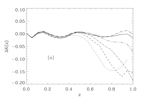
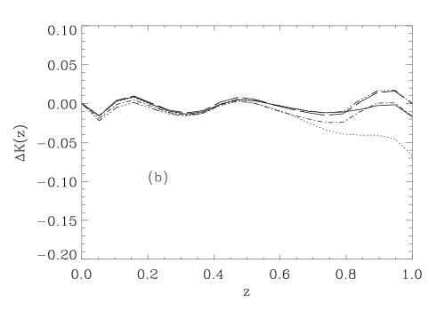
Figure 3: The difference between the default K band K–correction model of equation (1) and other models, generated using Bruzual & Charlot’s 1995 GISSEL library (see Charlot et al. 1996), all using a Salpeter (1955) IMF and mass range $0.1\leq M/M_{\odot}\leq 125$ unless otherwise stated: the oscillating form of these $\Delta K(z)$ curves is caused by the use of Chebyshev polynomials to produce the fit given in equation (1). In (a) we consider bursts of star formation of 1 Gyr duration at $z_{\rm f}=$ 1 (dotted line), 1.25 (dashed line), 1.5 (dot-dashed line), 2 (dot-dot-dot-dashed line), 3 (solid lines) and 4 (long-dashed lines): the $K(z)$ curve does not change significantly for $z_{\rm f}>4$. In (b) we show bursts at $z_{\rm f}=3$ with: (i) 1 Gyr duration (solid line, as in (a)); (ii) exponential decaying star formation rate with $\tau=1$ Gyr (dotted line); (iii) instantaneous burst (dashed line); (iv) instantaneous burst with mass range $0.1\leq M/M_{\odot}\leq 2.5$ (long-dashed line); (v) instantaneous burst with Scalo (1986) IMF (dot-dashed line); and (vi) instantaneous burst with Miller & Scalo (1979) IMF (dot-dot-dot-dashed line). We assume $\Omega_{\rm M}=1,\;\Omega_{\Lambda}=0$ and $h=0.5$ in all cases.The pronounced dips in $K(z)$ at $z$=0.7–1.0 for $z_{\rm f}$= 1.0–1.5 are caused by AGB stars: their appearance is short-lived, and pushed to $z>1$ if $z_{\rm f}\geq 1.5$. We only have one BCG at $z>0.6$, so their effect on our results will be negligible.

To illustrate the insensitivity of K band K–corrections to star formation history we show in Fig. 3 the difference between the default model of equation (1) and the $K(z)$ curves resulting from (a) varying $z_{\rm f}$, and (b) varying the IMF and form of the burst of star formation. It is clear that the age of the stellar population is the most important factor in determining the K–correction, but the variation of the K–correction with age only becomes noticable above $z\sim 0.4$, and is pushed to higher redshifts as $z_{\rm f}$ increases: as long as the bulk of a galaxy’s stars were formed before $z_{\rm f}=1.0$, then its K–correction is known to 0.05 or better if its redshift is $z\leq 0.6$ (we only have one BCG more distant than that) and known to that accuracy out to $z\sim 0.8$ if $z_{\rm f}>1.5$. Fig. 3 (b) shows that $K(z)$ is very insensitive to the IMF and duration of the burst of star formation.

If we convert the apparent magnitudes in Fig. 2 to absolute magnitudes, $M_{\rm K}$, using the K-correction model of equation (1) then the K-corrected mean absolute magnitude of the full 47 galaxy sample is $\bar{M}_{\rm K}=-26.40$ mag, and the rms dispersion about that mean is $\sigma=0.47$ mag. If we consider the higher-redshift half of the sample, (i.e. the 23 galaxies with $z>0.227$) then these figures become $\bar{M}_{\rm K}=-26.53$ mag and $\sigma=0.30$: this reduction in the rms dispersion in $\bar{M}_{\rm K}$ is significant at the 98.6 per cent level, since only 1399 out of 10⁵ 23-galaxy random subsamples of the full BCG sample give $\sigma$ values less than 0.30. Rather than assuming that the BCGs were formed at a single redshift, $z_{\rm f}$, we could follow Glazebrook et al. (1995) and assume that the stellar populations of our BCGs are of a constant age, irrespective of the redshift at which they are observed: that procedure leads to very similar results as those of the K–correction of equation (1) as the age of the BCGs is varied over the range $\sim 1-10$ Gyr (Glazebrook et al. 1995). The constant $z_{\rm f}$ and constant age assumptions both represent crude treatments of the star formation history of our BCGs, but the essential point here is that the very weak dependence of $K(z)$ to the exact formation redshift or exact age illustrates how insensitive near-infrared K–corrections are to the details of the star formation history of galaxies, and, hence, show the power of K band observations of early-type galaxies with a narrow intrinsic spread in absolute magnitude to act as standard candles.

It might be objected that the passive evolution models discussed in this Section are not appropriate for BCGs, since they might have experienced more recent star formation, either due to cooling flow activity or merging with other cluster galaxies. Allen (1995) studied six cooling flow clusters, finding large UV/blue continua and strong emission-lines, such as ${\rm H}\alpha$ and $[{\rm OII}]$, which can be interpreted as emission from O stars. In order to test for ongoing star formation we have examined the difference in absolute magnitudes between the EMSS BCGs in our sample which show some evidence for star-forming activity in their nucleus and the rest. From the EMSS cluster catalogue (Gioia & Luppino 1994) the BCGs in MS0302.7, MS0419.0, MS0537.1, MS0839.8, MS0955.7, MS1004.2, MS1125.3, MS1224.7 and MS1455.0 all have $[{\rm OII}]$, while MS0015.9 has many galaxies with “E+A” type spectra. Despite this, all ten lie very close to the mean Hubble relation shown in Fig. 2. A two-sided K-S test for BCGs in our sample with and without strong emission lines yields a probability of 0.17 that the difference in absolute magnitudes between the two populations would arise if the two subsamples are drawn from the same parent population. This result suggests that the effect of any ongoing star formation in the centres of BCGs on the K band magnitudes integrated over the 50 kpc diameter aperture is small. Such an interpretation of the spatial extent of any star formation in these systems is consistent with a number of studies which have concluded that optical colour gradients, indicative of active star formation, are either completely absent in BCGs (Andreon et al. 1992) or are confined to their inner regions (McNamara & O’Connell 1992).

Some BCGs are radio galaxies, so another possible concern is that some of the K band light from our BCGs comes from AGN, rather than from stars (Eales et al. 1997, and references therein). Gioia & Luppino (1994) list radio detections for only ten of the BCGs in our sample, and only six of these are in the high X-ray luminosity clusters in which we shall be particularly interested: a K-S test for the absolute magnitude distributions of our BCGs in high X-ray luminosity clusters yields a probability of 0.78 that BCGs with and without radio detections are drawn from the same parent population.

To summarise, there is no evidence to suggest we should not interpret the K band photometry of our BCGs as arising from the passive evolution of a mature stellar population formed at $z\ga 3$ similar to that advocated by Ellis et al. (1997) and others for cluster ellipticals in general. We shall, therefore, adopt equation (1) as our preferred K–correction, but will return, in Section 8, to discuss the effect that varying this assumed $K(z)$ relation has on the constraints on $\Omega_{\rm M}$ and $\Omega_{\Lambda}$ we deduce from the BCG Hubble diagfram.

5 PROPERTIES OF BCGS AND THEIR HOST CLUSTERS

The scatter in the raw Hubble diagram shown in Fig. 2 should come as no surprise, since it is well known that there exist strong correlations between the optical luminosities of BCGs and properties both of themselves, and of their host clusters, and that it is only after correction for these that BCGs are revealed to be good standard candles. In this Section we investigate some of the physical properties of the BCGs and their host clusters likely to be correlated with BCG luminosity.

5.1 The BCG structure parameter

Sandage (1972a,b) found that the luminosities of BCGs correlate with the richnesses and Bautz-Morgan (Bautz & Morgan 1970) type of their host clusters, and Hoessel (1980) showed how this could be expressed as a correlation between $L_{\rm m}$, the BCG luminosity within a metric aperture of radius $r_{\rm m}$, and $\alpha\equiv[{\rm d}\log(L_{\rm m})/{\rm d}\log(r)]|_{r=r_{\rm m}}$, the logarithmic slope of the BCG growth curve. Correction for the correlation with the structure parameter, $\alpha$, greatly reduces the dispersion in BCG absolute magnitudes, and the $L_{\rm m}-\alpha$ relation forms the basis of the recent use of BCGs as streaming velocity probes (Lauer & Postman 1994; Postman & Lauer 1995; Hudson & Ebeling 1997).

To measure the structure parameters of our BCGs, we computed the growth curve for each BCG from luminosity measurements in a set of apertures with radii increasing in steps of 1 pixel out to 100 pixels or 30 arcsec. Each curve was then modelled using a Hermite polynomial, which was fitted over the full range of the growth curve. The value of $\alpha$ was then determined for each BCG by evaluating the logarithmic derivative of the polynomial fit to its growth curve at an angle $\theta_{\rm m}$, which corresponds to a radius $r_{\rm m}=25$ kpc, and is given by

$$\theta_{\rm m}(\rm{arcsec})=0.43\frac{(1+z)^{2}}{[1-(1+z)^{-1/2}]},$$ (2)

for our assumed cosmology, with $\Omega_{\rm M}=1$, $\Omega_{\Lambda}=0$ and $h=0.5$. There are three principal sources of potential systematic error in our $\alpha$ estimates:

1. Incorrect background subtraction. In all cases, our galaxies are small enough that an adequate portion of uncontaminated image was available to estimate the sky level. We estimated what effect residual variations in the sky background have on the estimated structure parameter by recalculating the sky level using more than one uncontaminated part of each image. These tests were carried out on a random subset of 28 BCGs in our sample. The results indicated that uncertainties in sky subraction give rise to typical 1$\sigma$ errors of about 0.06 which is $\sim 10$ per cent on average: this dominates the uncertainty in the estimation of the structure parameter.

2. The presence of contaminating sources within the metric aperture. For 7 sources a star or second galaxy was found to lie within the circle corresponding to a projected distance of 25 kpc from the centre of the BCG. In these cases the contaminating sources were masked out, and the values of the pixels in the masked region, (which, in all cases, were close to 25 kpc away from the BCG), were replaced with the value of the pixel located at the same distance from the BCG but diametrically opposite the contaminating source. In tests with non-contaminated images, this process introduced very little additional error.

   Table 1: Seeing disk convolution results: the mean increase in $\alpha$ for two values of $r_{\rm m}$, as a function of redshift.

   $r_{\rm m}$	mean $\Delta\alpha$	mean $\Delta\alpha$	mean $\Delta\alpha$
   (kpc)	$0.2<z\leq 0.3$	$0.3<z\leq 0.4$	$0.4<z<0.8$
   8	0.04	0.05	0.10
   25	0.02	0.01	0.03

3. Profile broadening due to seeing. In the inner region of the BCG growth curves, the broadening effect of seeing causes the $\alpha$ values to be systematically overestimated. Over the course of our observations the seeing varied between 0.9 and 1.4 arcsec, with a median seeing of 1.1 arcsec: a seeing disk of this size is equivalent to a physical size of 5 kpc at $z=0.2$ and 8 kpc at $z=0.5$. To investigate the size of this effect we smoothed our images by convolving them with a Gaussian filter with a FWHM of 1.1 arcsec and re-measured the structure parameters. The mean increase in the measured $\alpha$ parameter computed at $r_{\rm m}=8h^{-1}$ kpc and $r_{\rm m}=25h^{-1}$ kpc in redshift bins is shown in Table 1. It is clear from Table 1 that the estimated corrections to the $\alpha$ parameter measured in a 50 kpc diameter aperture are small compared to other uncertainties, and there is little variation with redshift, so it is not necessary to correct our data for the effects of seeing. The advantages of using a larger aperture can also be seen, since the systematic corrections are significantly smaller for a 50 kpc aperture compared with those for a 16 kpc aperture. The adopted $\alpha$ values for our BCGs are tabulated in Table 2.

5.2 Host cluster X-ray luminosities

Hudson & Ebeling (1997) have recently argued that the residuals in the $L_{\rm m}-\alpha$ relation correlate with the X-ray luminosity of the host cluster, so that the $L_{\rm m}-\alpha$ relation does not fully remove the environmental dependence on BCG luminosity: the potential use of the cluster X-ray luminosity and/or temperature in reducing the scatter in the BCG Hubble diagram was also discussed by Edge (1991). In Table 2 we list the X-ray luminosities of the host clusters of our BCG sample. The EMSS X-ray luminosities for the 45 EMSS clusters are taken from Gioia & Luppino (1994), and are quoted for the energy pass band of the Imaging Proportional Counter ($0.3-3.5$ keV). We supplement that information with the luminosities for two ROSAT clusters (R84155 and R843053) which were discovered as part of an investigation of large-scale structure in the southern hemisphere (see Romer et al. 1994). The X-ray luminosities of these additional clusters have been corrected for extinction by using Hi column densities interpolated from Stark et al. (1992), then K-corrected and transformed from the ROSAT Position Sensitive Proportional Counter energy pass band ($0.1-2.4$ keV) to the EMSS energy range assuming a 6 keV thermal bremsstrahlung spectrum: the pass band correction is of the form $L_{\rm X}(0.3-3.5\;{\rm keV})=1.08\times L_{\rm X}(0.1-2.4\;{\rm keV})$.

Table 2: Data for the BCGs in the X-ray cluster sample

Cluster	RA	dec	z	$L_{\rm X}$	$m_{\rm BCG}$	$A_{K}$	$\alpha$	$N$	$\hat{N}$
MS0007.2-3532	00h07m14$\aas@@fstack{s}$5	-35°33′11$\aas@@fstack{\prime\prime}$8	0.050	0.517	11.14	0.01	0.49	0	-0.50
MS0015.9+1609	00h15m58$\aas@@fstack{s}$3	+16°09′34$\aas@@fstack{\prime\prime}$0	0.546	14.639	15.58	0.03	0.57	5	3.15
MS0301.7+1516	03h01m43$\aas@@fstack{s}$3	+15°15′50$\aas@@fstack{\prime\prime}$6	0.083	0.330	12.33	0.08	0.43	0	-1.00
MS0302.5+1717	03h02m29$\aas@@fstack{s}$4	+17°16′47$\aas@@fstack{\prime\prime}$6	0.425	2.879	14.65	0.07	0.75	5	3.89
MS0302.7+1658	03h02m43$\aas@@fstack{s}$2	+16°58′27$\aas@@fstack{\prime\prime}$0	0.426	5.043	15.01	0.07	0.67	4	2.51
MS0419.0-3848	04h18m59$\aas@@fstack{s}$6	-38°49′01$\aas@@fstack{\prime\prime}$2	0.225	0.385	14.67	0.01	0.32	0	-2.36
MS0433.9+0957	04h33m58$\aas@@fstack{s}$4	+09°57′36$\aas@@fstack{\prime\prime}$7	0.159	4.335	13.11	0.10	0.67	4	3.14
MS0451.6-0305	04h51m40$\aas@@fstack{s}$5	-03°05′46$\aas@@fstack{\prime\prime}$0	0.55	19.976	15.74	0.03	0.61	6	3.94
MS0537.1-2834	05h37m06$\aas@@fstack{s}$8	-28°34′40$\aas@@fstack{\prime\prime}$6	0.254	0.599	14.97	0.01	0.28	3	0.43
MS0821.5+0337	08h21m33$\aas@@fstack{s}$7	+03°37′30$\aas@@fstack{\prime\prime}$3	0.347	1.328	14.55	0.02	0.76	4	2.74
MS0839.8+2938	08h39m53$\aas@@fstack{s}$3	+29°38′16$\aas@@fstack{\prime\prime}$0	0.194	5.348	13.42	0.03	0.65	7	6.10
MS0849.7-0521	08h49m46$\aas@@fstack{s}$3	-05°21′36$\aas@@fstack{\prime\prime}$5	0.192	1.179	14.49	0.02	0.34	4	1.47
MS0904.5+1651	09h04m33$\aas@@fstack{s}$0	+16°51′15$\aas@@fstack{\prime\prime}$0	0.073	0.918	11.59	0.03	0.46	6	5.53
MS0906.5+1110	09h06m30$\aas@@fstack{s}$1	+11°10′39$\aas@@fstack{\prime\prime}$3	0.180	5.769	12.97	0.03	0.69	7	6.39
MS0955.7-2635	09h55m45$\aas@@fstack{s}$2	-26°35′56$\aas@@fstack{\prime\prime}$2	0.145	2.039	14.32	0.04	0.13	6	2.68
MS1004.2+1238	10h04m12$\aas@@fstack{s}$7	+12°38′15$\aas@@fstack{\prime\prime}$9	0.166	0.925	13.16	0.03	0.81	4	3.14
MS1006.0+1202	10h06m07$\aas@@fstack{s}$3	+12°02′20$\aas@@fstack{\prime\prime}$4	0.221	4.819	13.52	0.03	0.74	9	8.17
MS1008.1-1224	10h08m05$\aas@@fstack{s}$4	-12°25′07$\aas@@fstack{\prime\prime}$4	0.301	4.493	14.12	0.04	0.73	8	7.17
MS1054.4-0321	10h54m26$\aas@@fstack{s}$9	-03°21′25$\aas@@fstack{\prime\prime}$3	0.823	9.281	16.14	0.03	0.70	8	5.85
MS1111.8-3754	11h11m49$\aas@@fstack{s}$8	-37°54′55$\aas@@fstack{\prime\prime}$8	0.129	4.325	12.16	0.07	0.70	2	1.61
MS1125.3+4324	11h25m17$\aas@@fstack{s}$9	+43°24′09$\aas@@fstack{\prime\prime}$5	0.181	0.756	14.94	0.02	0.23	3	-1.00
MS1127.7-1418	11h27m52$\aas@@fstack{s}$3	-14°18′19$\aas@@fstack{\prime\prime}$2	0.105	2.786	12.02	0.03	0.90	6	5.55
MS1147.3+1103	11h47m18$\aas@@fstack{s}$2	+11°03′15$\aas@@fstack{\prime\prime}$9	0.303	2.304	14.36	0.02	0.61	3	1.76
MS1208.7+3928	12h08m44$\aas@@fstack{s}$0	+39°28′19$\aas@@fstack{\prime\prime}$0	0.340	2.030	14.32	0.01	0.55	3	1.95
MS1224.7+2007	12h24m42$\aas@@fstack{s}$6	+20°07′30$\aas@@fstack{\prime\prime}$0	0.327	4.606	14.61	0.02	0.62	1	-0.41
MS1241.5+1710	12h41m31$\aas@@fstack{s}$6	+17°10′06$\aas@@fstack{\prime\prime}$7	0.312	3.411	14.56	0.01	0.44	5	3.57
MS1253.9+0456	12h53m54$\aas@@fstack{s}$1	+04°56′25$\aas@@fstack{\prime\prime}$7	0.230	3.143	13.66	0.01	0.56	4	3.09
MS1426.4+0158	14h26m26$\aas@@fstack{s}$7	+01°58′36$\aas@@fstack{\prime\prime}$9	0.320	3.707	14.77	0.02	0.58	4	2.35
MS1455.0+2232	14h55m00$\aas@@fstack{s}$5	+22°32′34$\aas@@fstack{\prime\prime}$7	0.259	16.029	13.91	0.02	0.56	3	2.01
MS1512.4+3647	15h12m25$\aas@@fstack{s}$9	+36°47′26$\aas@@fstack{\prime\prime}$7	0.372	4.807	14.95	0.01	0.82	8	6.38
MS1522.0+3003	15h22m03$\aas@@fstack{s}$6	+30°03′51$\aas@@fstack{\prime\prime}$1	0.116	2.347	12.36	0.01	0.53	7	6.41
MS1531.2+3118	15h31m14$\aas@@fstack{s}$1	+31°18′42$\aas@@fstack{\prime\prime}$2	0.067	0.444	12.07	0.02	0.35	5	3.95
MS1532.5+0130	15h32m29$\aas@@fstack{s}$4	+01°30′46$\aas@@fstack{\prime\prime}$3	0.320	1.641	14.80	0.03	0.36	3	1.31
MS1546.8+1132	15h46m52$\aas@@fstack{s}$0	+11°32′25$\aas@@fstack{\prime\prime}$6	0.226	2.937	13.52	0.03	0.52	4	3.19
MS1558.5+3321	15h58m26$\aas@@fstack{s}$9	+33°21′40$\aas@@fstack{\prime\prime}$7	0.088	1.420	12.33	0.02	0.77	7	6.10
MS1617.1+3237	16h17m08$\aas@@fstack{s}$8	+32°37′52$\aas@@fstack{\prime\prime}$6	0.274	1.185	14.22	0.01	0.79	6	4.76
MS1618.9+2552	16h18m56$\aas@@fstack{s}$7	+25°53′22$\aas@@fstack{\prime\prime}$3	0.161	2.241	13.77	0.03	0.94	7	5.31
MS1621.5+2640	16h21m32$\aas@@fstack{s}$2	+26°41′06$\aas@@fstack{\prime\prime}$4	0.426	4.546	14.96	0.03	0.32	5	3.57
MS2053.7-0449	20h53m44$\aas@@fstack{s}$0	-04°49′24$\aas@@fstack{\prime\prime}$7	0.583	5.775	15.96	0.03	0.51	4	1.70
MS2124.7-2206	21h24m39$\aas@@fstack{s}$4	-22°07′15$\aas@@fstack{\prime\prime}$2	0.113	1.161	12.05	0.03	0.57	4	3.58
MS2215.7-0404	22h15m41$\aas@@fstack{s}$3	-04°04′25$\aas@@fstack{\prime\prime}$2	0.090	1.196	12.63	0.04	0.60	4	2.75
MS2216.0-0401	22h16m04$\aas@@fstack{s}$7	-04°01′51$\aas@@fstack{\prime\prime}$9	0.090	1.935	12.23	0.04	0.93	5	4.23
MS2255.7+2039	22h55m40$\aas@@fstack{s}$7	+20°39′04$\aas@@fstack{\prime\prime}$2	0.288	2.041	14.37	0.04	0.62	8	6.67
MS2301.3+1506	23h01m17$\aas@@fstack{s}$1	+15°06′49$\aas@@fstack{\prime\prime}$8	0.247	3.291	13.75	0.04	0.52	3	2.10
MS2354.4-3502	23h54m25$\aas@@fstack{s}$9	-35°02′15$\aas@@fstack{\prime\prime}$8	0.046	0.392	10.49	0.01	0.51	1	0.78
R84155	01h42m20$\aas@@fstack{s}$2	-22°28′39$\aas@@fstack{\prime\prime}$8	0.278	6.97	13.85	0.01	0.55	5	4.14
R843053	23h47m47$\aas@@fstack{s}$7	-24°52′30$\aas@@fstack{\prime\prime}$9	0.193	3.28	13.73	0.01	0.42	0	-1.24

The names, positions, redshifts and X-ray luminosities of the EMSS clusters (with prefix MS) are taken from Gioia & Luppino (1994): the RAs and decs. are given in B1950 coordinates and refer to the brightest cluster member in the $V$ band; and the X-ray luminosities, $L_{\rm X}$, are in units of 10⁴⁴ erg s^-1. $m_{\rm BCG}$ is the BCG K band magnitude within a 50 kpc diameter aperture, $A_{K}$ is the K band extinction correction (computed using the $N_{\rm H{\sc i}}$ maps of Stark et al. 1992, $R_{\rm V}=3.5$ and the mean extinction law of Mathis 1990), $\alpha$ is the structure parameter at 50 kpc diameter, while $N$ and $\hat{N}$ are, respectively, the raw and corrected BCG near neighbour numbers. Clusters commonly known by another name are as follows: MS0015.9+1609 (Cl0016+16); MS0839.8+2938 (Zwicky 1883); MS0904.5+1651 (Abell 744); MS0906.5+1110 (Abell 750); MS1006.0+1202 (Zwicky 2933); MS1127.7-1418 (Abell 1285); MS1253.9+0456 (Zwicky 5587); MS1522.0+3003 (Abell 2069); MS1531.2+3118 (Abell 2092); MS1558.5+3321 (Abell 2145); MS1618.9+2552 (Abell 2177); MS2255.7+2039 (Zwicky 8795); MS2301.3+1506 (Zwicky 8822); MS2354.4-3502 (Abell 4059); and R84155 (Abell 2938)

5.3 Near neighbour analysis

To test how well the correlations with $\alpha$ and $L_{\rm X}$ can express the environmental dependences of the BCG absolute magnitude, we wanted also to study residual dependences on the richness of the host cluster. Since our principal goal was to measure BCG magnitudes, we did not image more of the host clusters than fell into the field of view of the chip while imaging the BCG itself. In the most extreme case, this means we can only count near neighbours out to a distance of 100 kpc from the BCG: this means that we are looking at the central core of the cluster, rather than determining the richness of the cluster as a whole, for which one would want to count neighbours to some appreciable fraction of an Abell (1958) radius.

We used the starlink pisa package (Draper & Eaton 1996) to detect near neighbours within a projected distance of 100 kpc of the BCG centre, by searching for sets of at least ten contiguous pixels lying at least 2$\sigma$ above the sky level and used the iraf apphot package to estimate their magnitudes: we removed ‘obvious’ bright stars and foreground galaxies by eye, although few BCGs had one of these falling within the counting circle. From the sky noise level in each frame we were able to deduce its limiting isophote, which we converted into a limiting magnitude. We then computed, for each frame, the magnitude difference between the 50 kpc BCG magnitude and the limiting magnitude for that frame, finding that all frames went at least 4.66 magnitudes deeper than the BCG magnitude. Our raw near neighbour count for each BCG, $N$, was then taken to be the number of objects lying within a projected distance of 100 kpc of the BCG and with a magnitude less than 4.5 magnitudes fainter than the 50 kpc aperture magnitude of the BCG.

Figure 4: K band field galaxy count data. The solid line plots the fourth-order polynomial fit made to the count data, and used to predict the background count for each BCG. The symbols for the galaxy counts are as follows: diamonds, Mobasher et al. (1986); empty stars, Gardner et al. (1993); filled triangles, Glazebrook et al. (1994); crosses, Djorgovski et al. (1995); squares, McLeod et al. (1995); circles, Metcalfe et al. (1996); filled stars, Huang et al. (1997); and empty triangles, Gardner et al. (1997).

Figure 5: The K–$z$ diagram from Fig. 2 showing the location of members of quartiles in $\alpha$: the first quartile is shown by the squares, the second by the diamonds, the third by the triangles and the fourth by the circles.

Figure 6: The K–$z$ diagram from Fig. 2 showing the location of members of quartiles in $L_{\rm X}$: the first quartile is shown by the squares, the second by the diamonds, the third by the triangles and the fourth by the circles.

Figure 7: The K–$z$ diagram from Fig. 2 showing the location of members of quartiles in $\hat{N}$: the first quartile is shown by the squares, the second by the diamonds, the third by the triangles and the fourth by the circles.

We then estimated, for each BCG, the number of field galaxies expected to fall within the 100 kpc counting circle and the 4.5 mag magnitude strip. This was done using a fit to a compilation of K band galaxy count data kindly provided by J. Gardner (private communication), which comprises data from a number of authors: Mobasher et al. (1986), Gardner et al. (1993), Glazebrook et al. (1994), Djorgovski et al. (1995), McLeod et al. (1995), Metcalfe et al. (1996), Huang et al. (1997) and Gardner et al. (1997). These data are shown in Fig. 4, together with the following fourth order polynomial fit to them:

$$\log_{10}(\langle N(K)\rangle)\;=\;a_{0}+a_{1}K+a_{2}K^{2}+a_{3}K^{3}+a_{4}K^{4},$$ (3)

over the range $11.25\la K\la 23.5$, where $\langle N(K)\rangle$ is the expected galaxy count per mag per degree² at magnitude $K$, and the values of the coefficients in eqn (3) are as follows: $a_{0}=26.509$, $a_{1}=-8.3590$, $a_{2}=0.86876$, $a_{3}=-3.5824\times 10^{-2}$ and $a_{4}=5.2630\times 10^{-4}$. This fit has $\chi^{2}=128$ for 56 degrees of freedom and this is improved only marginally by increasing the order of the fit to tenth, say. In Table 2 we tabulate, for each BCG, the raw count $N$ and the corrected count, $\hat{N}$, obtained from it by subtracting the model background count. In six cases we find that the estimated contamination exceeds the raw count $N$: this is not unexpected, given the uncertainty in the background counts near the limiting magnitudes of the frames (which are, typically, $20\la K\la 21$) and our neglect of clustering in the background population, etc.

6 CORRELATING BCG AND HOST CLUSTER PROPERTIES

The correlations between BCG and host cluster properties are graphically illustrated by Figs. 5, 6 and 7, which show, on the Hubble diagram of Fig. 2, the members of the quartiles of, respectively, $\alpha$, $L_{\rm X}$ and $\hat{N}$. The similarity between these three figures shows how all these quantities are broad indicators of cluster richness, and, in particular, how the fainter BCGs at $z\la 0.25$ tend to be low $\alpha$ galaxies in poor systems, as defined both by the X-ray luminosity, $L_{\rm X}$, and by the near neighbour number, $\hat{N}$. This suggests that there would be redundancy in correcting the $K-z$ relation for all three quantities, so, in this Section, we perform a non-parametric correlation analysis (using the Spearman rank correlation coefficient, e.g. Press et al. 1992), to study the relationship between BCGs and their host clusters and, hence, to determine the best way to correct the BCG Hubble diagram for the effects of environment. We consider the five properties tabulated in Table 2: (i) redshift, $z$; (ii) absolute K band magnitude, $M_{\rm K}$, computed using the K-correction model of equation (1); (iii) X-ray luminosity, $L_{\rm X}$; (iv) corrected near neighbour number, $\hat{N}$; and (v) BCG structure parameter, $\alpha$.

Table 3: Results of Spearman rank correlation analysis. The upper half of the table gives the Spearman rank correlation coefficient, $r_{\rm AB}$, while the lower half gives $\hat{P}_{\rm AB}\equiv-\log_{\rm 10}[P(r_{\rm AB})]$, where $P(r_{\rm AB})$ is the probability that the absolute value of the correlation coefficient would be as large as $|r_{\rm AB}|$ for a sample of the same size, under the hypothesis that the quantities $A$ and $B$ are uncorrelated.

	$z$	$M_{\rm K}$	$L_{\rm X}$	$\hat{N}$	$\alpha$
$z$	-	-0.22	0.61	0.02	0.10
$M_{\rm K}$	0.86	-	-0.49	-0.39	-0.40
$L_{\rm X}$	5.36	3.29	-	0.34	0.31
$\hat{N}$	0.04	2.15	1.74	-	0.58
$\alpha$	0.28	2.29	1.49	4.73	-

In Table 3 we present the results of this Spearman rank correlation analysis: in the upper half of the table we tabulate the Spearman rank correlation coefficient, $r_{\rm AB}$, while the lower half gives $\hat{P}_{\rm AB}\equiv-\log_{\rm 10}[P(r_{\rm AB})]$, where $P(r_{\rm AB})$ is the probability that the absolute value of the correlation coefficient would be as large as $|r_{\rm AB}|$ for a sample of the same size, under the hypothesis that the quantities $A$ and $B$ are uncorrelated. The $P(r_{\rm AB})$ values are computed under the assumption that the quantity $r_{\rm AB}[(N-2)/(1-r_{\rm AB}^{2})]^{1/2}$, where $N$ is the number of galaxies in the sample, is distributed like Student’s t statistic: from Monte Carlo simulations we judge this approximation to be very good, typically estimating $\hat{P}_{\rm AB}$ to an accuracy of $\sim$0.02. A very similar set of results to Table 3 is obtained if we use either the constant age K-correction of Glazebrook et al. (1995) or the empirical K-correction of Aragón–Salamanca et al. (1993), rather than the model fit of equation (1). Note that the use of a rank correlation coefficient underestimates the true level of correlation between $M_{\rm K}$ and $\alpha$ to the extent that this relation is parabolic, as commonly assumed, rather than monotonic (see Section 7 below): none of the other relations tabulated in Table 3 are so affected, justifying our use of a rank correlation analysis to quantify them.

Figure 8: Correlation of $\hat{N}$ and $\alpha$. This relation is not simply the result of contamination within a radius $r_{\rm m}$ of the BCG, since these objects were removed before calculating $\alpha$.

A number of these correlations are worthy of comment. Firstly, the K band absolute magnitudes of our BCGs show no evidence of significant evolution with redshift, above the passive evolution removed by the K-correction, but we see from Table 3 that $M_{\rm K}$ is strongly correlated with $L_{\rm X}$, $\hat{N}$ and $\alpha$. The strong correlation between $z$ and $L_{\rm X}$ simply reflects the flux-limited nature of EMSS cluster sample, but note that the strong correlation between $\hat{N}$ and $\alpha$ (shown in Fig. 8) is not due to near neighbours lying within $r_{\rm m}$ of the BCG, since we explicitly excluded such contamination in calculating $\alpha$: instead, it illustrates how well $\alpha$ can express the richness of the BCG’s local environment, as argued by Hoessel (1980).

These results could, of course, be due to correlations with a third quantity: for example, we know that $\hat{N}$ and $\alpha$ are strongly correlated, so the correlation between $\hat{N}$ and $M_{\rm K}$, say, could just result from that and a correlation between $M_{\rm K}$ and $\alpha$. To test that we have computed, for our five physical properties, partial Spearman correlation coefficients (e.g. Yates et al. 1986) of the form $r_{\rm AB,C}$, where

$$r_{\rm AB,C}\;=\;\frac{r_{\rm AB}-r_{\rm AC}r_{\rm BC}}{[(1-r^{2}_{\rm AC})(1-r^{2}_{\rm BC})]^{1/2}},$$ (4)

where $r_{\rm AB}$, etc, are the Spearman rank correlation coefficients, as before. The significance of the partial rank correlation coefficients may be calculated using a similar approximation as above – that $r_{\rm AB,C}[(N-3)/(1-r_{\rm AB,C}^{2})]^{1/2}$ is distributed as Student’s t statistic – to compute the probability, $P(r_{\rm AB,C})$, of obtaining a partial rank correlation coefficient with absolute value as large as $|r_{\rm AB,C}|$ under the null hypothesis that the correlation between $A$ and $B$ results solely from correlations between $A$ and $C$ and between $B$ and $C$: Monte Carlo simulations show that this approximation works as well for $P(r_{\rm AB,C})$ as for $P(r_{\rm AB})$.

We relegate the full set of partial rank correlation results to an Appendix, and note only a few important points here. The most striking result is that once the dependence on X-ray luminosity has been removed, $\alpha$ becomes independent of $z$ to a high degree: $P(r_{\rm z\alpha,L_{\rm X}})=0.60$. We find that the $\hat{N}-\alpha$ relation is not due to separate correlations between those two variables and a third: the lowest $P(r_{\rm AB,C})$ for $A=\hat{N}$ and $B=\alpha$ arises when $C=M_{\rm K}$, but, even then, there is a probability of less than $4\times 10^{-4}$ that the $\hat{N}-\alpha$ correlation is entirely due to the $M_{\rm K}-\hat{N}$ and $M_{\rm K}-\alpha$ correlations. This leads to high values of $P(r_{\rm AB,C})$ when $A=\hat{N}$ and $C=\alpha$, or vice versa, since these variables are almost interchangable. There is some reduction in the significance of the $M_{\rm K}-L_{\rm X}$ correlation when it is evaluated at constant $\alpha$, but it remains quite strong, consistent with the suggestion by Hudson & Ebeling (1997) that correction for $L_{\rm X}$ can remove some of the residual environmental dependence of BCG magnitudes left after the $L_{\rm m}-\alpha$ correction has been made. Finally, it appears that none of the significant correlations between pairs of properties arise from separate evolutionary trends of the properties with redshift. To summarise, it is clear that $M_{\rm K}$ is strongly correlated with both $\alpha$ and $L_{\rm X}$, and that no further correction for $\hat{N}$ need be made after the $\alpha$-correction, due to the strength of the correlation between $\hat{N}$ and $\alpha$.

7 THE CORRECTED K-$\mn@boldsymbol{z}$ RELATION

The relationship between absolute magnitude and $\alpha$ for our BCG sample is shown in Fig. 9. The relationship diverges from a purely linear slope at large values of $\alpha$ and is in this respect qualitatively similar to those of Hoessel (1980), who used a sample of 108 Abell clusters, and Postman & Lauer (1995), who determined $\alpha$ for a sample of 119 BCGs at $z\leq 0.05$ in the R band. In a similar way to Postman & Lauer (1995), we fit the correlation between structure parameter and K band luminosity with a parabola, which gives a least-squares best fit of

$$M_{\rm K}=-23.84-(8.34\pm 1.14)\alpha+(6.14\pm 1.00)\alpha^{2},$$ (5)

which is also shown in Fig. 9. The vertical scatter about this fit is $\sigma=0.29$ mag, and the gradient in the linear part of the relation is significantly steeper for our sample than for the R band sample of Postman & Lauer (1995). It is clear that a parabolic fit is a reasonable description of the data over the range $0.1\leq\alpha\leq 1.0$, and Fig. 9 provides the first real evidence that the $L_{\rm m}-\alpha$ relation at least flattens at high $\alpha$, rather than continuing linearly with increased scatter, as appears the case for the Postman & Lauer (1995) data.

Figure 9: The $L_{\rm m}-\alpha$ relation for our data set. The filled and empty squares denote the BCGs in clusters with X-ray luminosities greater than and less than $2.3\times 10^{44}$ erg s^-1 respectively. The line shows the best quadratic fit to the data.

Figure 10: The relationship between X-ray luminosity and raw BCG absolute magnitude. The empty squares denote the BCGs in clusters with $L_{\rm X}<2.3\times 10^{44}$ erg s^-1, while the filled squares are the BCGs in clusters above that threshold. Note the much wider spread of absolute magnitudes seen for the BCGs in the less X-ray-luminous clusters.

Figure 11: The relationship between X-ray luminosity and $\alpha$-corrected BCG absolute magnitude. The empty squares denote the BCGs in clusters with $L_{\rm X}<2.3\times 10^{44}$ erg s^-1, while the filled squares are the BCGs in clusters above that threshold. Comparison of this plot and Fig. 10 shows how the $\alpha$ correction removes most of the scatter in the absolute magnitudes of the low-$L_{\rm X}$ BCGs, while leaving the high-$L_{\rm X}$ ones virtually unchanged.

The filled squares in Fig. 9 are the BCGs in high-$L_{\rm X}$ clusters. Note that these are all to be found near the peak of the parabola, indicating how high-$L_{\rm X}$ selection picks out BCGs with a narrow range of absolute magnitudes, and suggesting that these magnitudes will be largely unaffected by the correcting for the $M_{\rm K}-\alpha$ relation of equation (5). This is graphically demonstrated by Figs. 10 and 11, which show, respectively, the relationship between $L_{\rm X}$ and the raw and $\alpha$-corrected $M_{\rm K}$ values. Below host cluster X-ray luminosities of $L_{\rm X}\simeq 2.3\times 10^{44}$ erg s^-1, there is a wide dispersion in raw BCG absolute magnitudes, which is largely, but not completely, removed by the $M_{\rm K}-\alpha$ correction, while the high-$L_{\rm X}$ absolute magnitudes are barely changed. In what follows we use this threshold of $L_{\rm X}=2.3\times 10^{44}$ erg s^-1 to mark the break between a homogeneous population of BCGs in high-$L_{\rm X}$ and a low-$L_{\rm X}$ population which displays a wider scatter in its properties. Intriguingly, the $L_{\rm X}$ threshold we empirically found on the basis of BCG properties is almost identical to that Annis (1997) has recently argued marks the dividing point in the X-ray properties of EMSS clusters: above $2\times 10^{44}$ erg s^-1 the X-ray properties are very homogeneous, while below that, Annis detects two populations of clusters, with quite differing properties, one of which he argues contains clusters where the X-ray emission is solely from the intracluster medium (the only sort of cluster found above $2\times 10^{44}$ erg s^-1) and the other where a significant contribution comes from a cooling flow. We note that the lack of strong correlation between $M_{\rm K}$ and $\alpha$ for high $L_{\rm X}$ clusters found here, is in contrast to the results found by Hudson & Ebeling (1997), who argue that the optical $L_{\rm m}-\alpha$ relation actually steepens for high-$L_{\rm X}$ Abell clusters. However, their local Abell sample does not probe luminosities as high as the EMSS clusters – only 2 clusters in their sample have $L_{\rm X}\geq 2.3\times 10^{44}$ erg s^-1 in the EMSS passband.

After correction for the $M_{\rm K}-\alpha$ relation of equation (5) we find that the rms dispersion in absolute magnitudes falls from $\sigma=0.47$ mag to $\sigma=0.29$ magnitudes, while the dispersion for the high-$L_{\rm X}$ subsample (the 26 galaxies in clusters with $L_{\rm X}>2.3\times 10^{44}$ erg s^-1) about its own best-fit $M_{\rm K}-\alpha$ relation is 0.22 mag, identical to the rms dispersion in their raw magnitudes: the best-fit relation for the high-$L_{\rm X}$ sample is $M_{\rm K}=-26.18-(0.87\pm 2.34)\alpha-(0.18\pm 1.89)\alpha^{2}$, indicating the weakness of the dependence of $M_{\rm K}$ on $\alpha$ shown in Fig. 9 for these BCGs.

The residuals about the best $M_{\rm K}-\alpha$ fit for the high-$L_{\rm X}$ sample do not correlate with $z$, $L_{\rm X}$ or $\hat{N}$, while, for the full sample, the only significant correlation is with $L_{\rm X}$, similar to that reported by Hudson & Ebeling (1997). We also tried correcting our raw absolute magnitudes using the same form of $L_{\rm m}-\alpha-L_{\rm X}$ relation recently advocated by Hudson & Ebeling (1997) which, translated to the K band, reads

$$M_{\rm K} = c_{0}+c_{1}\alpha+c_{2}\alpha^{2}+c_{3}\log_{10}(\hat{L}_{\rm X})+c_{4}\alpha\log_{10}(\hat{L}_{\rm X})$$ (6)

$$+ c_{5}\alpha^{2}\log_{10}(\hat{L}_{\rm X}),$$

where $\hat{L}_{\rm X}$ is the cluster X-ray luminosity in units of $10^{44}$ erg s^-1. For the full sample, the best fit values of these parameters are $c_{0}=-23.26$, $c_{1}=-10.66\pm 1.58$, $c_{2}=8.45\pm 1.49$, $c_{3}=-3.63\pm 1.13$, $c_{4}=12.23\pm 4.30$ and $c_{5}=-10.37\pm 3.97$, which means that the terms are in similar proportion to those found by Hudson & Ebeling (1997) for the Lauer & Postman (1994) optical BCG sample. With this model, the rms dispersion of the full sample is decreased slightly to 0.26 mag, while that for the high-$L_{\rm X}$ sample actually increases slightly to 0.23 mag, as the loss of degrees of freedom arising from the use of three more parameters in the fit outweighs the marginal decrease in the scatter in absolute magnitudes brought about by correction for the residual dependence on $L_{\rm X}$ left after correction for $\alpha$.

In principle, galaxy merging in the centre of clusters should increase the stellar mass of the BCGs with time. Hausman & Ostriker (1978) show that the $\alpha$ parameter is a sensitive measure of the merging history of BCGs: therefore, we can determine the effect that the merging process has had on our sample by using the $\alpha$ parameter as a tracer of the growth of the BCGs through merging. As the Spearman results of Section 6 for the full sample show, once the dependences of $\alpha$ on $L_{\rm X}$ and of $L_{\rm X}$ on $z$ are removed, $\alpha$ is independent of $z$: there is a 60 per cent probability that the correlation between $\alpha$ and $z$ arises from the combination of their individual correlations with $L_{\rm X}$. This lack of a correlation between $\alpha$ and $z$ is slightly more strongly confirmed for the high-$L_{\rm X}$ sample of 26 BCGs, as the Spearman test for a correlation between $\alpha$ and $z$ for these galaxies gives a correlation coefficient with probability of 0.63 of arising from uncorrelated variables. We conclude, therefore, that the BCGs in the high-$L_{\rm X}$ clusters sample form a very homogeneous population, with an intrinsic dispersion in absolute magnitude of no more than 0.22 mag, and that there has been no significant evolution due to galaxy merging since a redshift of $z\sim 0.8$. It follows that our high-$L_{\rm X}$ BCG sample constitute a set of standard candles ideal for use in classical cosmological tests, such as the estimation of $\Omega_{\rm M}$ and $\Omega_{\Lambda}$.

8 ESTIMATING $\Omega_{\rm M}$ AND $\Omega_{\Lambda}$ FROM THE BCG HUBBLE DIAGRAM

The Hubble diagram for a set of standard candles determines the relationship between luminosity distance, $d_{\rm L}$, and redshift, which may be written (Carroll, Press & Turner 1992; Perlmutter et al. 1997) in the general form

$$d_{\rm L}(z,\Omega_{\rm M},\Omega_{\Lambda},H_{0})=\frac{c(1+z)}{H_{0}\sqrt{|\kappa}|}\times$$

$$\!\!{\cal I} \!\!\!\!\!\!\left\{\!\!\sqrt{|\kappa|}\int_{0}^{z}\!\!dx\left[(1+x)^{2}(1+\Omega_{\rm M}x)-x(2+x)\Omega_{\Lambda}\right]^{-1/2}\right\}$$ (7)

where: (i) if $\Omega_{\rm M}+\Omega_{\Lambda}>1$, then ${\cal I}(x)=\sin(x)$ and $\kappa=1-\Omega_{\rm M}-\Omega_{\Lambda}$; (ii) if $\Omega_{\rm M}+\Omega_{\Lambda}<1$, then ${\cal I}(x)=\sinh(x)$ and $\kappa=1-\Omega_{\rm M}-\Omega_{\Lambda}$; and (iii) if $\Omega_{\rm M}+\Omega_{\Lambda}=1$, then ${\cal I}(x)=x$ and $\kappa=1$. As emphasised by Perlmutter et al. (1997), it is important to note that the form of equation (7) means that $d_{\rm L}$ depends on $\Omega_{\rm M}$ and $\Omega_{\Lambda}$ independently, and not solely through the deceleration parameter, $q_{0}\equiv\Omega_{\rm M}/2-\Omega_{\Lambda}$ – i.e. the confidence region in the $(\Omega_{\rm M},\Omega_{\Lambda})$ plane determined from the Hubble diagram of a set of standard candles is not parallel to contours of constant $q_{0}$, except at $z\ll 1$. We prefer, therefore, to solve for $\Omega_{\rm M}$ and $\Omega_{\Lambda}$ using our Hubble diagram for BCGs in high-$L_{\rm X}$ clusters, rather than for $q_{0}$.

We do that, using the following procedure for each candidate cosmology:

1. Select values for $\Omega_{\rm M}$ and $\Omega_{\Lambda}$: $h=0.5$ is assumed throughout.

2. Using equation (7), compute the angle, $\theta_{\rm m}$, corresponding to a physical distance $r_{\rm m}=25$ kpc at the redshift of each of the 47 BCGs: $\theta_{\rm m}=r_{\rm m}/d_{\rm A}$, where $d_{\rm A}=d_{\rm L}/(1+z)^{2}$ is the angular diameter distance.

3. Calculate the change in the apparent magnitudes of the BCGs, as $\Delta m_{\rm BCG}=\alpha(d_{\rm A}-d_{\rm A,ref})/d_{\rm A,ref}$, where the $\alpha$ values are those in Table 2, which assume $\Omega_{\rm M}=1$ and $\Omega_{\Lambda}=0$, and $d_{\rm A,ref}$ is the angular diameter distance in that reference model. This first order correction to the apparent magnitude should be accurate so long as $r_{\rm m}$ does not vary much from the reference aperture with $\Omega_{\rm M}=1$ and $\Omega_{\Lambda}=0$, and that condition holds true for all physically reasonable cosmologies.

4. Compute the ages of the galaxies in the cosmology, assuming their formation at a redshift $z_{\rm f}=3$, and compute their K–corrections using the Bruzual & Charlot models, as described in Section 4. Use the K-corrections for, and luminosity distances of, the galaxies in the cosmology to derive the BCG absolute magnitudes.

5. Perform a quadratic fit to the new $M_{\rm K}-\alpha$ relation, and use it to correct the BCG magnitudes to a fiducial $\alpha$ value, which is taken to be the median $\alpha$.

6. Take the mean of the $\alpha$-corrected $M_{\rm K}$ as the estimate for $M_{0}$, the BCG K band absolute magnitude, and deduce its standard error, from the scatter of the $M_{\rm K}$ values about $M_{0}$.

7. For the redshifts of the 26 BCGs in high-$L_{\rm X}$ clusters, calculate the predicted apparent magnitude, given $M_{0}$ and the $K(z)$ relation in the cosmology. Using the errors on the measured magnitudes of the 26 BCGs in high-$L_{\rm X}$ clusters, and the standard error on $M_{0}$, compute $\chi^{2}$ for the comparison of the 26 BCG apparent magnitudes and the apparent magnitudes predicted at their redshifts in the cosmology.

We report these results for two classes of cosmology, with and without a cosmological constant.

8.1 Friedmann models: $\Omega_{\Lambda}=0$

Figure 12: The joint constraints on the value of $\Omega_{\rm M}$ and the BCG formation redshift $z_{\rm f}$ deduced from the Hubble diagram for the BCGs in our high–$L_{\rm X}$ clusters. The dotted line shows the locus of the best-fit $\Omega_{\rm M}$ value for one hundred values of $z_{\rm f}$ in the range $1\leq z_{\rm f}\leq 10$, while the solid contours mark the 68, 95 and 99 per cent confidence contours for $\Omega_{\rm M}$ and $z_{\rm f}$: the small amplitude random fluctuations in the dotted line are numerical artefacts introduced by our method of estimating $\Omega_{\rm M}$, while the behaviour of all the curves in the range $1.25\leq z\leq 2.25$ is caused by the transient presence of light from AGB stars in the stellar synthesis model used to compute the BCG K-corrections, as discussed in Section 4.

Much of the previous work trying to estimate cosmological parameters from the Hubble diagrams of distant galaxies has assumed $\Omega_{\Lambda}=0$, in which case the deceleration parameter, $q_{0}$, is given by $q_{0}=\Omega_{\rm M}/2$. Table 4 summarises the $q_{0}$ values obtained previously, from a variety of galaxy samples, using BCGs and radio galaxies, in both the optical and the near-infrared. Several points are worthy of note, motivating the use of K band photometry of BCGs in X-ray clusters to estimate $q_{0}$. Firstly, as discussed above, the use of K band photometry is to be preferred to the use of optical photometry, due to the insensitivity of K band light to star formation history of the galaxy. This means that our estimated $q_{0}$ value is insensitive to uncertainties in the age of the stellar population of the BCGs and in the stellar IMF: optical photometry would produce a greater uncertainty in $q_{0}$ on both those scores. Secondly, X-ray cluster selection is to be preferred over optical cluster selection, since, as we have shown, it is very effective at selecting galaxies with a very narrow intrinsic dispersion in absolute magnitude. Thirdly, BCGs are to be preferred over radio galaxies, both because the intrinsic dispersion in radio galaxy absolute magnitudes appears larger ($\sim 0.5$ mag) and because bias may be introduced by the significant non-stellar component to the K band light (Dunlop & Peacock 1993; Eales et al. 1997).

If we assume $\Omega_{\Lambda}=0$, then we obtain $\Omega_{\rm M}=0.28\pm 0.24$ if $z_{\rm f}=3$. Consistent values are obtained if $z_{\rm f}$ is varied between $z_{\rm f}=1$ (i.e. slightly higher than the redshift of our most distant BCG) to $z_{\rm f}=10$, as shown in Fig. 12. These results are consistent with the results of Perlmutter et al. (1997), who find $\Omega_{\rm M}=0.88^{+0.69}_{-0.60}$ for a $\Omega_{\Lambda}=0$ cosmology, from the Hubble diagram of the first seven high-$z$ Type Ia supernovae discovered by The Supernova Cosmology Project (although our best-fit $\Omega_{\rm M}$ value is clearly lower than theirs, and our confidence interval is much narrower) and with those of Carlberg et al. (1996), who find $\Omega_{\rm M}\simeq 0.24\pm 0.09$ from CNOC cluster mass profiles.

Table 4: Previous estimates of the deceleration parameter $q_{0}$ from the Hubble diagram of BCGs and radio galaxies. The symbols in the waveband column denote whether the measurements were carried out in the optical (O) or near-infrared (IR). Wherever possible the $q_{0}$ values listed are those quoted by the authors after correcting for evolution, otherwise the raw values are given.

Sample	$z$ range	Waveband	Number	$q_{0}$	Reference
BCG	$\leq 0.2$	O	17	$2.5\pm 1.0$	Humason, Mayall & Sandage (1956)
BCG	$\leq 0.46$	O	8	$1.0\pm 0.5$	Baum (1957, 1961a,b)
BCG	$\leq 0.46$	O	38	$1.5\pm 0.9$	Peach (1970)
BCG	$0.003-0.46$	O	84	$0.96\pm 0.4$	Sandage (1972b)
BCG	$0.005-0.46$	O	98	$1\pm 1$	Sandage & Hardy (1973)
BCG	$0.01-0.47$	O	68	$0.33$ or $-1.27$	Gunn & Oke (1975)
BCG	$0.04-0.46$	O	67	$1.0\pm 0.3$	Sandage, Kristian & Westphal (1976)
BCG	$0.04-0.75$	O	50	$1.6\pm 0.4$	Kristian, Sandage & Westphal (1978)
radio	$0.14-0.95$	IR	6	$\simeq 0$	Lebofsky (1980)
radio	$0.03-1.6$	IR	83	$0-0.6$	Lilly & Longair (1984)
radio	$0.016-0.9$	IR	61	$\simeq 0.5$	Lebofsky & Eisenhardt (1986)
BCG	$0.017-0.147$	O	116	$-0.55\pm 0.45$	Hoessel, Gunn & Thuan (1980)
BCG	$0.15-0.83$	O	41	$0.3\pm(0.21-0.39)$	Clowe, Luppino & Gioia (1995)
X-ray BCG	$0.11-0.83$	IR	26	$0.14\pm 0.12$	this work

8.2 Friedmann-Lemaître models: $\Omega_{\Lambda}\neq 0$

Figure 13: The joint constraints on $\Omega_{\rm M}$ and $\Omega_{\Lambda}$ obtainable from the Hubble diagram of the 26 BCGs in high-$L_{\rm X}$ clusters. The contours mark the 68, 90 and 95 per cent confidence levels for $\Omega_{\rm M}$ and $\Omega_{\Lambda}$ jointly, while the the dashed and dotted lines mark the models with $\Omega_{\Lambda}=0$ and $\Omega_{\rm M}+\Omega_{\Lambda}=1$ respectively.

Fig. 13 shows the joint constraints on $\Omega_{\rm M}$ and $\Omega_{\Lambda}$ we obtain if we allow a non-zero cosmological constant: this is very similar to the corresponding plot presented by Perlmutter et al. (1997). If we consider only spatially flat models, where $\Omega_{\rm M}+\Omega_{\Lambda}=1$, we find $\Omega_{\rm M}=0.55^{+0.14}_{-0.15}$, with a corresponding 95 per cent upper limit to $\Omega_{\Lambda}$ of 0.73, for $z_{\rm f}=3$: as above, these figures are very stable, varying marginally over the full range $z_{\rm f}\leq 10$. Perlmutter et al. (1997) find $\Omega_{\rm M}=0.94^{+0.34}_{-0.28}$ if they assume a spatially flat Universe, which is again consistent with our results: their results translate into a 95 per cent confidence level of $\Omega_{\Lambda}<0.51$, slightly tighter than ours. From the incidence of gravitational lensing of quasars, Kochanek (1996) derived a 95 per cent limit of $\Omega_{\Lambda}<0.66$, while two recent studies have reported significant detections of non-zero $\Omega_{\Lambda}$ values: Henry (1997) finds $\Omega_{\rm M}=0.55\pm 0.17$ from the evolution of the cluster X-ray temperature function, and Bender et al. (1997) deduce $\Omega_{\rm M}\sim 0.5$, $\Omega_{\Lambda}\sim 0.5$ from cluster elliptical Fundamental Plane relations.

9 DISCUSSION AND CONCLUSIONS

This paper has presented the K band Hubble diagram for a sample of BCGs in X-ray selected clusters. Our principal results are that the brightest X-ray clusters contain BCGs with a very narrow spread of absolute magnitudes, and that this, coupled with the insensitivity of K band light to the details of the star formation processes in, and histories of, galaxies, makes samples such as ours ideal for performing classical cosmological tests. We find that the BCGs in the clusters with high X-ray luminosities ($L_{\rm X}>2.3\times 10^{44}$ erg s^-1 in the 0.3 - 3.5 keV passband) have an rms dispersion in absolute K band magnitude of no more than 0.22 mag, and that leads us to an estimate of $\Omega_{\rm M}=0.28\pm 0.24$ if $\Lambda=0$, while, for a spatially flat Universe, we find $\Omega_{\rm M}=0.55\pm 0.15$ and a 95 per cent limit of $\Omega_{\Lambda}<0.73$, with only a very weak sensitivity to the properties of the stellar population of the BCGs over a wide range of redshifts. The stability of these results demonstrates that BCGs are excellent standard candles, competitive with Type Ia supernovae (which also have an intrinsic magnitude dispersion of $\sim 0.2$ mag: Perlmutter et al. 1997) in the estimation of cosmological parameters $\Omega_{\rm M}$ and $\Omega_{\Lambda}$: the further refinement of these two techniques over the next few years holds out hope for the determination of these fundamental cosmological parameters with high precision.

Finally, the lack of evolution we see in the K band, shown by the absence of a correlation between the BCG structure parameter, $\alpha$, and redshift, adds to the growing body of evidence that cluster ellipticals are old systems, possibly undergoing only quiescent evolution of their stellar populations (e.g. Dunlop et al. 1996; Bender et al. 1996; Ellis et al. 1997). It is intriguing to note that a qualitatively similar lack of evolution is seen in the X-ray luminosity (Collins et al. 1997, Burke et al. 1997) and temperature (Mushotsky & Scharf 1997, Henry 1997) functions. We shall return to this question of the relationship between the formation and evolution of BCGs and their host clusters in a forthcoming paper, incorporating recently acquired K band imaging data for BCGs in clusters from the deep Southern SHARC ROSAT cluster survey (Collins et al. 1997): these clusters were selected above a flux limit an order of magnitude fainter than that of the EMSS, enabling us to disentangle the effects of redshift and X-ray luminosity, in a manner impossible with the current data set.

REFERENCES

Abell G.O., 1958, ApJS, 3, 211

Allen S.W., 1995, MNRAS, 276, 947

Andreon S., Garilli B., Maccagni D., Vettolani G., 1992, AA, 266, 127

Annis J., 1997, preprint

Aragón-Salamanca A., Ellis R., Couch W.J., Carter D., 1993, MNRAS, 262, 794

Baum W.A., 1957, AJ, 62, 6

Baum W.A., 1961a, Observatory, 81, 114

Baum W.A., 1961b, in McVittie G.C., ed, Proc. IAU Symp. 15. MacMillan, New York, p. 390

Bautz L.P., Morgan W.W., 1970, ApJ, 162, L149

Bender R., Saglia, R.P., Ziegler, B., Belloni, P., Greggio, L., Hopp, U., 1997, ApJ, in press

Bender R., Ziegler B., Bruzual G., 1996, ApJ, 463, L51

Bershady M.A., Hereld M., Kron R.G., Koo D.C., Munn J.A., Majewski S.R., 1994, AJ, 108, 870

Bershady M.A., 1995, AJ, 109, 87

Bruzual A.G., Charlot S., 1993, ApJ, 405, 538

Burke D.J., Collins, C.A., Sharples, R.M., Romer, A.K., Holden, B.P., Nichol R.C., 1997, ApJ, 488, L83

Carlberg R.G., et al., 1996, ApJ, 462, 32

Carroll S.M., Press, W.H., Turner, E.L., 1992, ARAA, 30, 499

Casali M.M., Hawarden T.G., 1992, JCMT-UKIRT Newsletter, no. 3, 33

Charlot S., Worthey G., Bressan A., 1996, ApJ, 457, 625

Clowe D., Luppino G., Gioia I.M, 1995, in Trimble V., Reisenegger A., ed, Clusters, Lensing, and the Future of the Universe, Vol. 88

Collins C.A., Burke D.J., Romer A.K., Sharples R.M., Nichol R.C., 1997, ApJ, 479, L117

Djorgovski S.G., Soifer B.T., Pahre M.A., Larkin J.E., Smith J.D., Neugebauer G., Smail I., Matthews K., Hogg D.W., Blandford R.D., Cohen J., Harrison W., Nelson J., 1995, ApJ, 438, L13

Draper P.W., Eaton N., 1996, pisa, Starlink User Note 109, http://star-www.rl.ac.uk/star/docs/sun109.htx /sun109.html

Dunlop J., Peacock J. A., 1993, MNRAS, 263, 936

Dunlop J., Peacock J., Spinrad H., Dey A., Jimenez R., Stern D., Windhorst, R., 1996, Nature, 381, 581

Eales S., et al., 1997, MNRAS, in press

Edge A.C., 1991, MNRAS, 250, 191

Ellis R.S. Smail I., Dressler A., Couch W.J., Oemler A., Butcher H., Sharples R.M., 1997, ApJ, 483, 582

Gardner J.P., Cowie L.L., Wainscoat R.J., 1993, ApJ, 415, L9

Gardner J.P., Sharples R.M., Carrasco B.E., Frenk C.S., 1997, MNRAS, in press

Glazebrook K., Peacock J.A., Collins C.A., Miller L., 1994, MNRAS, 266, 65

Glazebrook K., Peacock J.A., Miller L., Collins C.A., 1995, MNRAS, 275, 169

Gioia I.M., Maccacaro T., Schild R.E., Wolter A., Stocke J.T., Morris S.L. & Henry J.P. 1990, ApJS, 72, 567

Gioia I.M., Luppino G.A., 1994, ApJS, 94, 583

Gunn J.E., Oke J.B., 1975, ApJ, 195, 255

Haussman M.A., Ostriker J.P., 1978, ApJ, 224, 320

Henry J.P., 1997, preprint

Hoessel J.G., 1980, ApJ, 241, 493

Hoessel J.G., Gunn J.E., Thuan T.X., 1980, ApJ, 241, 486

Hoessel J.G., Schneider D.P., 1985, AJ, 90, 1648

Huang J.-S., Cowie L.L., Gardner J.P., Hu E.M., Songaila A., Wainscoat R.J., 1997, ApJ, in press

Hubble E., 1929, Proc. Nat. Acad. Sci. 15, 168

Hudson M.J., Ebeling H., 1997, ApJ, 479, 621

Humason M.L., Mayall N.U., Sandage A.R., 1956, AJ, 61, 97

Kochanek C.S., 1996, ApJ, 466, 638

Kristian J., Sandage A., Westphal J.A., 1978, ApJ, 221, 383

Lauer T.R., Postman M., 1994, ApJ, 425, 418

Lebofsky M.J., 1980, in Abell G.O., Peebles P.J.E., eds, Proc. IAU Symp. 92, Objects of High Redshift. Reidel, Dordrecht, p. 257

Lebofsky M.J., Eisenhardt P.R.M., 1986, ApJ, 300, 151

Lilly S.J., Longair M.S., 1984, MNRAS, 211, 833

Mathis J.S., 1990, ARAA, 28, 37

McLeod B.A., Bernstein G.M., Rieke M.J., Tollestrup E.V., Fazio G.G., 1995, ApJS, 96, 117

McNamara B.R., O’Connell R.W., 1992, ApJ, 393, 579

Metcalfe N., Shanks T., Campos A., Fong R., Gardner J.P., 1996, Nat, 383, 236

Miller G.E., Scalo J.M., 1979, ApJS, 41, 513

Mushotsky R.F., Scharf C.A., 1997, ApJ, in press

Mobasher B., Ellis R.S., Sharples R.M., 1986, MNRAS, 223, 11

Peach J.V., 1970, ApJ, 159, 753

Perlmutter S., et al., 1997, ApJ, 483, 565

Postman M., Lauer T., 1995, ApJ, 440, 28

Press W.H., Teukolsky S.A., Vetterling W.T., Flannery B.R., 1992, Numerical Recipies in FORTRAN, The Art of Scientific Computing, Second Edition, Cambridge University Press, Cambridge

Romer A.K., Collins C.A., Böhringer H., Cruddace R.G., Ebeling H., MacGillivray H.T., Voges W., 1994, Nature, 372, 75

Salpeter E.E., 1955, ApJ, 121, 161

Scalo J.M., 1986, FCPh, 11,1

Sandage A.R., 1972a, ApJ, 173, 485

Sandage A.R., 1972b, ApJ, 178, 1

Sandage A.R., 1988, ARA&A, 26, 561

Sandage A.R., 1995, in Binggeli B., Buser R., eds, The Deep Universe, Saas-Fee Advanced Course 23. Springer, Berlin, p. 3.

Sandage A.R., Hardy E., 1973, ApJ, 183, 743

Sandage A.R., Kristian J., Westphal J.A., 1976, ApJ, 205, 688

Stark A.A., Gammie C.F., Wilson R.W., Bally J., Linke R.A., Heiles C., Hurwitz M., 1992, ApJS, 79,77

Stocke J.T., Morris S.L., Gioia I.M., Maccacaro T., Schild R.E., Wolter A., Fleming T.A., Henry J.P. 1991, ApJS, 76, 813

Trümper J., 1993, Science, 260, 1769

van Haarlem M.P., Frenk C.S., White S.D.M., 1997, MNRAS, 287, 817

Voges W., 1992, Proceedings of Satellite Symposium 3, ESA ISY-3, p9

Yates M.G., Miller L., Peacock J.A., 1986, MNRAS, 221, 311

Appendix A PARTIAL SPEARMAN TEST RESULTS

In this Appendix we tabulate results from the partial Spearman rank correlation analysis of Section 5 that it would be too tedious to include in the main body of the text of this paper. The partial Spearman rank correlation coefficient $r_{\rm AB,C}$ (defined in equation 4 of Section 6) quantifies the strength of the correlation between $A$ and $B$, once the effect of their individual correlations with $C$ has been removed. The significance of $r_{\rm AB,C}$ may readily be computed. This is the probability, $P_{\rm AB,C}$, that a correlation coefficient with absolute value as high as $|r_{\rm AB,C}|$ would arise if the correlation between $A$ and $B$ arose solely from their separate correlations with $C$: in common with Yates et al. (1986), we find that Monte Carlo simulations indicate that this may be computed sufficiently accurately using the approximnation that $r_{\rm AB,C}[(N-3)/(1-r_{\rm AB,C}^{2})]^{1/2}$ is distributed as Student’s t statistic.

We tabulate here the $r_{\rm AB,C}$ values for the five quantities studied in Section 5: (i) redshift, $z$; (ii) absolute K band magnitude, $M_{\rm K}$, computed using the K-correction model of equation (1); (iii) X-ray luminosity, $L_{\rm X}$; (iv) corrected near neighbour number, $\hat{N}$; and (v) BCG structure parameter, $\alpha$. In each table, the upper half lists the partial Spearman rank correlation coefficient, $r_{\rm AB,C}$, while the lower half gives $\hat{P}_{\rm AB,C}\equiv-\log_{\rm 10}[P(r_{\rm AB,C})]$. We consider the effect of setting $C$ equal to each of these in turn, by which we study the significance of correlations between pairs of variables $A$ and $B$ after removing the effect of correlations between $A$ and $C$ and between $B$ and $C$.

Table A1: Results of partial Spearman rank correlation analysis for constant redshift, i.e. $C=z$. The upper half of the table gives the values of $r_{\rm AB,C}$, while the lower half gives $\hat{P}_{\rm AB}\equiv-\log_{\rm 10}[P(r_{\rm AB,C})]$, where $P(r_{\rm AB,C})$ is the probability that the absolute value of the correlation coefficient would be as large as $|r_{\rm AB,C}|$ for a sample of the same size, under the hypothesis that the correlations between $A$ and $B$ arise solely from their individual correlations with $C$

	$z$	$M_{\rm K}$	$L_{\rm X}$	$\hat{N}$	$\alpha$
$z$	-	-	-	-	-
$M_{\rm K}$	-	-	-0.46	-0.39	-0.39
$L_{\rm X}$	-	2.86	-	0.42	0.32
$\hat{N}$	-	2.17	2.45	-	0.58
$\alpha$	-	2.15	1.54	4.67	-

Table A2: Results of partial Spearman rank correlation analysis for constant absolute magnitude, i.e. $C=M_{\rm K}$: format as for Table A1.

	$z$	$M_{\rm K}$	$L_{\rm X}$	$\hat{N}$	$\alpha$
$z$	-	-	0.60	-0.76	0.01
$M_{\rm K}$		-	-	-	-
$L_{\rm X}$	4.91	-	-	0.19	0.15
$\hat{N}$	0.21	-	0.69	-	0.50
$\alpha$	0.02	-	0.48	3.45	-

Table A3: Results of partial Spearman rank correlation analysis for constant X-ray luminosity, i.e. $C=L_{\rm X}$: format as for Table A1.

	$z$	$M_{\rm K}$	$L_{\rm X}$	$\hat{N}$	$\alpha$
$z$	-	0.12	-	-0.26	-0.13
$M_{\rm K}$	0.35	-	-	-0.27	-0.30
$L_{\rm X}$	-	-	-	-	-
$\hat{N}$	1.10	1.15	-	-	0.53
$\alpha$	0.40	1.37	-	3.84	-

Table A4: Results of partial Spearman rank correlation analysis for constant corrected near neighbour number, i.e. $C=\hat{N}$: format as for Table A1.

	$z$	$M_{\rm K}$	$L_{\rm X}$	$\hat{N}$	$\alpha$
$z$	-	-0.23	0.65	-	0.11
$M_{\rm K}$	0.92	-	-0.41	-	-0.23
$L_{\rm X}$	5.97	2.33	-	-	0.15
$\hat{N}$	-	-	-	-	-
$\alpha$	0.31	0.94	0.49	-	-

Table A5: Results of partial Spearman rank correlation analysis for constant structure parameter, i.e. $C=\alpha$: format as for Table A1.

	$z$	$M_{\rm K}$	$L_{\rm X}$	$\hat{N}$	$\alpha$
$z$	-	-0.20	0.62	-0.04	-
$M_{\rm K}$	0.74	-	-0.42	-0.21	-
$L_{\rm X}$	5.34	2.40	-	0.21	-
$\hat{N}$	0.12	0.78	0.79	-	-
$\alpha$	-	-	-	-	-