The Luminosity and Mass Function of the Globular Cluster NGC 1261

Abstract

I-band CCD images of two large regions of the Galactic globular cluster NGC 1261 have been used to construct stellar luminosity functions (LF) for 14000 stars in three annuli from $1\hbox{\hbox to0.0pt{\hbox{.}\hss}\hbox{${}^{\prime}$}}4$ from the cluster center to the tidal radius. The LFs extend to $M_{I}\sim 8$ and tend to steepen from the inner to the outer annulus, in agreement with the predictions of the multimass King–Michie model that we have calculated for this cluster. The LFs have been transformed into mass functions. Once corrected for mass segregation the global mass function of NGC 1261 has a slope $x_{0}=0.8\pm 0.5$

1 Introduction

One of the basic ingredients of a stellar system is the mass distribution of its population of stars. In the case of globular clusters (GCs), stellar mass functions (MFs) reflect both the initial conditions from the epoch of cluster formation and the dynamical evolution. In order to try to disentangle the effects of evolution from those of the initial conditions on the shapes of globular cluster MFs we have started a long-term project aimed at getting deep luminosity functions (LF) in a large sample of galactic GCs. The first results of this project have already been presented in other papers (cf. Piotto 1993 and Piotto et al. (1996) for a complete bibliography on recent works on GC LFs). Since Scalo (1986) it has been known that the MFs of Galactic GCs differ from cluster to cluster. McClure et al. (1986) proposed that the MF slopes depend on the cluster metallicity. By studying a sample of 17 Galactic GCs, Capaccioli, Ortolani, & Piotto (1991) questioned the hypothesis that the metal content could be the main parameter governing the MF shapes; instead, they showed that the position of the parent cluster within the Galactic gravitational potential is affecting the present day MFs (PDMF). By means of a more detailed statistical analysis on the same sample of Capaccioli et al. (1991), Djorgovski, Piotto, & Capaccioli (1993) demonstrated that the MF slopes are determined both by the positional variables and by the metallicity. The two positional variables are dominant, with similar but not equivalent effects: at a given Galactocentric distance $R_{GC}$, clusters with a smaller distance from the galactic plane $Z_{GP}$ have shallower MFs, and vice-versa. However, they do not determine the MF completely: at a given position, clusters with higher metallicity have shallower MFs. This dependence on the positional coordinates has been tentatively interpreted as the effect of selective evaporation of stars, driven by tidal shocks (Capaccioli, Piotto, & Stiavelli 1993): heating due to disk shocking acts preferentially on stars located in the outer regions of the cluster and, in combination with mass segregation, it leads to a loss of low mass stars, i.e. to a MF flattening. The dependence on the metallicity could reflect the initial conditions. This scenario has been furtherly confirmed by recent HST data (Piotto, Cool, & King 1997) which allowed to extend the study of GC MFs almost down to the limit of the core hydrogen-burning ignition ($\sim 0.1M_{\odot}$).

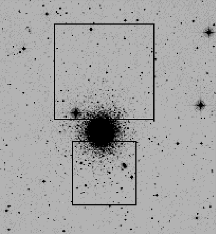
Figure 1: The two fields observed in NGC 1261: the upper one is the NTT field, while the lower box shows the 2.2m field

In this paper we present I-band stellar luminosity functions of NGC $1261=$C$0310-554$, a cluster which is presently relatively far from the center and the plane of the Galaxy. On the basis of the location of NGC 1261 within the Galaxy, $R_{GC}=17.8$ kpc and $Z_{GP}=12.6$ kpc, it is very likely that its evolution has been driven more by the internal dynamics rather than by strong tidal shocks. For this reason, despite its large distance from the Sun, NGC 1261 has been chosen (among other clusters) for a detailed study of the PDMF, which should be as close as the internal dynamical evolution can allow to the initial MF (IMF).

NGC 1261 ($\alpha_{2000}=3^{h}12^{m}15^{s}$, $\delta_{2000}=-55^{\circ}13^{\prime}1^{{}^{\prime\prime}}$; is a medium concentration globular cluster ($c=1.27$ Trager, King and Djorgovski 1995), located at high galactic latitude, $l=250\hbox{\hbox to0.0pt{\hbox{.}\hss}\raise 5.0pt\hbox{{\small$\circ$}}}54$, $b=-52\hbox{\hbox to0.0pt{\hbox{.}\hss}\raise 5.0pt\hbox{{\small$\circ$}}}13$. Its low reddening and small field star contamination make it a very good target for photometric studies. The first CCD color–magnitude diagram (CMD) for NGC 1261 has been published by Bolte & Marleau (1989). They observed the cluster in $B$ and $V$, down to magnitude $V\sim 23$. From the apparent magnitude of the HB and the fitting of the main sequence to two subdwarfs, they derived an apparent distance modulus $(m-M)_{V}=16.05\pm 0.25$. By matching their observations to the VandenBerg and Bell (1985) isochrones and assuming E(B-V)=0.02, Bolte and Marleau obtained an age of 15 Gyr and a metallicity [M/H]=–1.09. By adopting E(B–V)=0.04, the best fitting isochrone gives an age of 15 Gyr and a metallicity [M/H]=–1.27.

Alcaino et al. (1992) published a $BVR$ photometric study of NGC 1261. They found a distance modulus $(m-M)_{V}=16.00\pm 0.23$, from the apparent magnitude of the HB, and, using the same set of isochrones of the previous study, an age of $15\pm 2$ Gyr, and a reddening of E(B-V)$=0.07$, assuming a metallicity [Fe/H]$=-1.27$. More recently, Ferraro et al. (1993) presented a $BV$ CMD and a luminosity function for the evolved stars in this cluster. From the CMD metallicity indicators, calibrated with the Zinn & West (1984) metallicity scale, they estimated a slightly lower metal content than in the previous studies: [Fe/H]$=-1.4\pm 0.2$. They also detected for the first time the ‘RGB bump’ of the cluster, as a clump of stars in the LF of the red giant branch, at magnitude $V=16.70\pm 0.05$.

The paper is organized as follows: in Section 2 we discuss our data and the method we followed to obtain the photometry. In Section 3 we present the luminosity functions in three radial annuli. Section 4 concerns the mass functions and the correction for the effects of the mass segregation. Finally, in the last Section the MF of NGC 1261 is compared with the MFs for other 19 Galactic GCs.

Figure 2: This plot shows the difference between the magnitude at which each artificial star was added to the image and the magnitude at which it was found, as a function of the input magnitude. The graphic refers to the artificial-star experiments on the NTT frame. The horizontal and vertical dashed lines are the limits of the LF magnitude bin (i.e. a star that falls out from the two horizontal lines at $\pm 0.250$ would have been counted in the previous or in the next LF magnitude bin.

2 Observation and data reduction

The database consists of two I–band image sets. The first one is a sample of seven 15 min exposures obtained on November 27–30, 1991, with EFOSC2 + CCD # 17 at the ESO/MPI 2.2 m telescope of La Silla. These images have dimensions of $1024\times 1024$ pixels, corresponding to an area of 5.^′8$\times$5.^′8 on the sky, and cover a region from $\sim 1\hbox{\hbox to0.0pt{\hbox{.}\hss}\hbox{${}^{\prime}$}}4$ to $\sim 7\hbox{\hbox to0.0pt{\hbox{.}\hss}\hbox{${}^{\prime}$}}0$ from the center of the cluster. The second set consists of 9 frames, for a total exposure time of 95 minutes, obtained with EMMI + CCD # 34 at the ESO/NTT telescope in December 1993. This field cover $9\hbox{\hbox to0.0pt{\hbox{.}\hss}\hbox{${}^{\prime}$}}6\times 8\hbox{\hbox to0.0pt{\hbox{.}\hss}\hbox{${}^{\prime}$}}5$ of the sky, from $\sim 1\hbox{\hbox to0.0pt{\hbox{.}\hss}\hbox{${}^{\prime}$}}2$ to $\sim 9\hbox{\hbox to0.0pt{\hbox{.}\hss}\hbox{${}^{\prime}$}}5$ from the center, as shown in Fig. 1. All observations have been taken in fairly good seeing conditions ($<FWHM>\sim 1\hbox{\hbox to0.0pt{\hbox{.}\hss}\hbox{${}^{\prime\prime}$}}0$).

Figure 3: The position of the stars present in the field observed with EMMI and the radial annuli in which we separated the counts. The inner annulus has boundaries $1\hbox{\hbox to0.0pt{\hbox{.}\hss}\hbox{${}^{\prime}$}}4\leq r<2\hbox{\hbox to0.0pt{\hbox{.}\hss}\hbox{${}^{\prime}$}}5$, the intermediate one has $2\hbox{\hbox to0.0pt{\hbox{.}\hss}\hbox{${}^{\prime}$}}5\leq r<4\hbox{\hbox to0.0pt{\hbox{.}\hss}\hbox{${}^{\prime}$}}0$, and the outer annulus has $4\hbox{\hbox to0.0pt{\hbox{.}\hss}\hbox{${}^{\prime}$}}0\leq r<8\hbox{\hbox to0.0pt{\hbox{.}\hss}\hbox{${}^{\prime}$}}0$

Figure 4: Same as Fig. 3, for the field observed with EFOSC2

The images were bias-corrected, trimmed and flat-fielded with routines in MIDAS. The single frames of the same field were averaged in order to increase the signal-to-noise ratio. Profile-fitting photometry of stars was performed with DAOPHOT II (Stetson 1987).

In order to obtain deep luminosity functions it is necessary to measure the magnitudes of very faint stars with good accuracy. This can be dangerous if one has frames only in one photometric band, because in this case it is very difficult to identify and reject spurious detections. For EMMI images we minimized this problem by averaging separately two sets of frames: a first set of five images (say image A) and a second one of four images (image B). The stellar photometry on these two images has been done independently from each other. The star list used as input for the photometry on images A and B was the final list of objects resulting from the complete photometry of the median image of all the (nine) original frames. This is the deepest image, as it has the highest signal-to-noise ratio. The final star catalog (used for the LFs) contains only the stars measured in both images A and B. The magnitude associated to each star is the average of the magnitudes we measured in the two images. This method allows to use the full information present in our data set and also to eliminate most of the spurious detections, as, in general, the noise peaks cannot be present in both images at the same position. Indeed, the probability that a pixel differs by more than 3.5 $\sigma$ from the average value of the sky is 0.0004; the probability that the $same$ pixel differs more than 3.5 $\sigma$ in both images is $1.6\times 10^{-7}$. Since our images have dimension of 1700$\times$1500 pixels, for a total of 2550000 pixels, we expect that 0.41 noise peaks should be present as spurious detections in our star list.

The completeness corrections have been estimated by standard artificial-star experiments. We performed 10 independent experiments per field, adding each time a total of 600 stars, with the spatial distribution of a King model of the same concentration (c=1.3, Trager et al. 1995) of NGC 1261. The finding algorithm adopted to recover and measure the artificial stars was the same used for the photometry of the original images. As discussed extensively by Stetson & Harris (1988) and Drukier et al. (1988), photometric errors cause the measured magnitude of an artificial star to be different from its input magnitude, just as “real” stars may have measured magnitudes different from their true magnitudes.

Table 1: NTT Luminosity Functions

$$\begin{array}[]{lllllll}\hline\cr\vskip 3.0pt plus 1.0pt minus 1.0pt\cr IMag&N_{inn}&N^{c}_{inn}&N_{int}&N^{c}_{int}&N_{out}&N^{c}_{out}\\ \vskip 3.0pt plus 1.0pt minus 1.0pt\cr\hline\cr\vskip 3.0pt plus 1.0pt minus 1.0pt\cr 16.75&2.9&2.9\pm 0.8&0.4&0.4\pm 0.2&-&-\\ 17.25&2.7&2.6\pm 0.8&0.5&0.4\pm 0.2&-&-\\ 17.75&2.9&2.9\pm 0.8&1.0&0.9\pm 0.3&0.2&0.1\pm 0.1\\ 18.25&5.6&5.5\pm 1.1&1.2&1.1\pm 0.3&0.4&0.3\pm 0.1\\ 18.75&6.7&6.6\pm 1.2&2.2&2.1\pm 0.4&0.4&0.3\pm 0.1\\ 19.25&22.2&22.0\pm 2.2&3.6&3.5\pm 0.5&0.7&0.6\pm 0.1\\ 19.75&47.9&46.9\pm 3.2&7.1&7.0\pm 0.8&0.9&0.8\pm 0.1\\ 20.25&62.9&62.8\pm 3.7&11.2&11.0\pm 0.9&2.1&2.0\pm 0.2\\ 20.75&86.2&126.7\pm 12.5&15.2&15.0\pm 1.4&3.3&3.1\pm 0.3\\ 21.25&94.1&94.8\pm 17.0&19.6&20.1\pm 1.6&4.8&4.2\pm 0.4\\ 21.75&96.3&136.7\pm 25.6&27.7&30.1\pm 2.3&6.4&5.9\pm 0.5\\ 22.25&74.1&164.9\pm 31.1&31.4&29.3\pm 3.1&8.9&8.1\pm 0.6\\ 22.75&-&-&31.8&42.7\pm 3.5&10.5&9.4\pm 0.8\\ 23.25&-&-&30.1&43.8\pm 5.9&11.5&11.5\pm 1.1\\ 23.75&-&-&-&-&8.6&12.1\pm 5.0\\ \vskip 3.0pt plus 1.0pt minus 1.0pt\cr\hline\cr\end{array}$$

Table 2: 2.2m Luminosity Functions

$$\begin{array}[]{lllllll}\hline\cr\vskip 3.0pt plus 1.0pt minus 1.0pt\cr IMag&N_{inn}&N^{c}_{inn}&N_{int}&N^{c}_{int}&N_{out}&N^{c}_{out}\\ \vskip 3.0pt plus 1.0pt minus 1.0pt\cr\hline\cr\vskip 3.0pt plus 1.0pt minus 1.0pt\cr 16.75&0.9&0.9\pm 0.5&0.6&0.6\pm 0.3&-&-\\ 17.25&2.5&2.4\pm 0.8&0.5&0.4\pm 0.2&-&-\\ 17.75&2.5&2.4\pm 0.8&0.8&0.8\pm 0.3&0.1&0.1\pm 0.1\\ 18.25&2.7&2.6\pm 0.8&1.8&1.7\pm 0.5&0.2&0.1\pm 0.1\\ 18.75&11.1&9.2\pm 2.7&2.8&2.8\pm 0.6&0.6&0.5\pm 0.2\\ 19.25&24.3&20.6\pm 9.9&7.6&7.0\pm 1.0&1.4&1.3\pm 0.3\\ 19.75&37.2&33.9\pm 18.0&13.6&11.4\pm 1.4&2.1&1.9\pm 0.3\\ 20.25&55.1&50.7\pm 27.5&20.8&20.7\pm 1.9&2.6&2.5\pm 0.4\\ 20.75&61.5&59.9\pm 20.3&27.0&24.7\pm 2.2&4.3&4.1\pm 0.5\\ 21.25&68.9&94.4\pm 27.5&35.6&33.6\pm 3.6&4.0&3.3\pm 0.8\\ 21.75&54.0&71.7\pm 24.5&39.6&43.3\pm 7.1&6.3&4.6\pm 1.3\\ 22.25&52.8&96.0\pm 25.5&36.1&44.8\pm 19.3&8.0&8.8\pm 2.3\\ 22.75&-&-&28.8&47.4\pm 22.6&8.0&9.6\pm 3.1\\ 23.25&-&-&-&-&6.4&11.0\pm 5.9\\ 23.75&-&-&-&-&-&-\\ \vskip 3.0pt plus 1.0pt minus 1.0pt\cr\hline\cr\end{array}$$

In general, the measured magnitude of a star is brighter than the input magnitude, as shown in Fig. 2 (see Stetson & Harris 1988 for a discussion on the origin of this phenomenon). A solution to this problem was suggested by Drukier et al. (1988): using the artificial–star data it is possible to set up a two dimensional matrix giving, for each input–magnitude bin, the probability that a star would appear in each output–magnitude bin. To be more explicit, the columns of the matrix represent the input magnitude bins and the rows represent the output. In this way, each matrix element contains the probability that a star added in the magnitude bin $i$ (row $i$) is found in the magnitude bin $j$ (column $j$). This probability is defined as the ratio of the number of artificial stars found in each magnitude bin (rows of the matrix) to the number of stars added in a bin (columns of the matrix). The inverse of this matrix gives the completeness correction factors. The observed LF, once multiplied by this inverse matrix, becomes the complete LF, with the two different effects of crowding properly corrected: the loss of stars and their migration in magnitude (cf. Drukier et al. 1988 for the details). In order to evaluate the uncertainty associated to each element of the completeness matrix, we performed nine independent experiments on each field, created nine matrices and inverted each of them separately, using the Gauss-Jordan elimination method. By calculating the mean value and its standard deviation for each element, we were able to determine the errors associated to the crowding correction.

Figure 5: Left panel: open circles the radial surface brightness profile of NGC 1261 by Trager et al. (1995). The points relative to our counts in the EMMI field (after completeness correction) are represented with filled circles. The fourth annulus (which is entirely outside the tidal radius given by Trager et al. ) has been divided into two sub-annuli. Here we note that the star counts monotonically decrease till the outer limit of our field, i.e. we never reach the background level, even if the last two points refer to stars which are all outside the tidal radius $r_{t}=7\hbox{\hbox to0.0pt{\hbox{.}\hss}\hbox{${}^{\prime}$}}3$ given by Trager et al. Right panel: comparison between the LF for the annulus outside the published tidal radius (filled circles) corresponding to the last two points in the left panel, and the background/foreground counts predicted by Ratnatunga & Bahcall (1985) for this region. The observed counts in the right panel are not corrected for completeness.

In order to calibrate the instrumental magnitudes to a standard system, during each observing night we observed 27 standard stars at the 2.2m and 18 standards at the NTT, in 4 Landolt (1992) standard fields. The calibration equations are:

$$I_{instr}-I=(0.04\pm 0.01)(V-I)+2.14\pm 0.01$$

for the 2.2m data, and:

$$I_{instr}-I=(0.004\pm 0.002)(V-I)+0.60\pm 0.01$$

for the NTT data. As we have no $V$-band image, we adopted a mean color $(V-I)=1.2$ for the main-sequence stars in the range of magnitudes we were studying (17$<M_{I}<$24). Since the total range in color spanned by this region of the main-sequence is $\Delta(V-I)$=0.8, the real color of our stars might be wrong by at most $\pm$0.4 magnitudes. Using the color term of the two equations above, this gives an error of $\Delta I=\pm 0.02$ for the 2.2m data, and $\Delta I=\pm 0.002$ for NTT. Considering also the error in the zero point, we have a total uncertainty $\Delta I=\pm 0.03$ for the 2.2m data and $\Delta I=\pm 0.01$ for the NTT data, negligible in both cases, in view of the fact that the LF bin is of 0.5 magnitudes.

3 Luminosity Functions

The luminosity function of a system is constructed by simply counting the number of stars in successive magnitude bins. We separated observed star counts in different radial annuli (see Figs. 3 and 4) in order to take into account the different effects of crowding at different distances from the center of the cluster. Moreover, by determining luminosity and mass functions at different radial distances we are able to study the effects of mass segregation (Section V).

For both the EMMI and the 2.2 m fields we separated the star counts in three annuli: the inner one, from $1\hbox{\hbox to0.0pt{\hbox{.}\hss}\hbox{${}^{\prime}$}}4$ to $2\hbox{\hbox to0.0pt{\hbox{.}\hss}\hbox{${}^{\prime}$}}5$, the intermediate one, from $2\hbox{\hbox to0.0pt{\hbox{.}\hss}\hbox{${}^{\prime}$}}5$ to $4^{\prime}$, and the external one, from $4^{\prime}$ to $8^{\prime}$. The stars in a fourth region of the NTT image, with $r>8^{\prime}$, have been used to check the background/foreground contamination. The dimensions of these annuli were chosen in order to have about the same statistical sample of stars and to avoid a significant crowding gradient inside each one. The latter condition ensured that we could apply just one completeness correction for each radial luminosity function.

A peculiarity of NGC 1261 is the fact that it lies on the line of sight to a cluster of galaxies. These galaxies were identified by DAOPHOT as agglomerates of stars. To solve this problem, we visually inspected the images and found the coordinates and the sizes of the galaxies directly on the frame, and then rejected all the stars within the galaxy boxes from the output file of ALLSTAR.

Figure 6: Comparison between the LFs of the two fields, for each radial annulus. Bottom to top: inner, intermediate and outer annulus.

Another source of contamination is given by the foreground/background stars that are projected on the cluster. Normally one can correct this effect by determining the luminosity function of a region of sky near the cluster (in order to have the same population of field stars) but far enough to be sure there is no cluster object. Then, one has simply to subtract the number of field stars per unit area and unit magnitude from the cluster LF. Our idea was to consider as a foreground field the region just outside the tidal radius of NGC 1261, in the EMMI field. As the published value of the tidal radius of NGC 1261 is $r_{t}=7^{\prime}.3$ (Trager et al. 1995), we isolated the stars outside $8^{\prime}$ from the center of the cluster, and determined their luminosity function. Unfortunately, a plot of the cumulative number of stars per unit area versus the distance from the center demonstrates that there is no flattening at the tidal radius, i.e. the value of $r_{t}$ seems to be underestimated (or, alternatively, there is a halo of cluster stars, beyond the tidal radius, as found by Grillmair et al. 1995 for other clusters). This fact is confirmed by Fig. 5 in which we represent (left panel) the surface brightness of NGC 1261 as a function of the radial distance. In this plot, the points coming from our counts in each annulus have been added to the data of Trager et al. (1995). The fourth annulus (which is entirely outside the tidal radius given by Trager et al. ) has been divided into two sub-annuli. It is clear that the surface brightness is still decreasing outside $r_{t}$, and we can not use the LF from the “external” annulus to correct for foreground/background contamination. As a further evidence, in the right panel of the same figure we compare the star counts observed in the region outside $8^{\prime}$ with the counts predicted by Ratnatunga & Bahcall (1985) model. Our counts are overabundant with respect to the expected foreground up to a factor of five, well outside the uncertainty given by Ratnatunga & Bahcall for their model. We conclude that all our fields lie entirely inside the boundary of the cluster. For this reason, the background/foreground correction has been done using the counts by Ratnatunga & Bahcall (1985) based on the Galaxy model by Bahcall & Soneira (1984). The amount of this correction is, at most, 10% of the original counts.

Figure 7: Total LFs for the three radial annuli. The counts have been normalized in the magnitude interval 17.3$<I<$20.5.

No correction is made here for the possible contamination of the LF by fainter, uresolved galaxies. However, a simple test was carried out to insure that, would a correction be made, the conclusion of this work would have been the same. We examined the CMD obtained from two sets of deep HST WFPC2 V and I images for the GCs M92 and M30, two clusters whose projected position in the Galaxy is similar to that of NGC 1261. We measured the number of foreground stars and galaxies for these clusters counting all the objects that lie outside $\pm 5\sigma$ from the cluster Main Sequence. We then scaled this counts to 1 arcmin² area and subtracted the number of object expected to be stars, given by Ratnatunga & Bahcall (1985). The number of remaining objects is our best estimate of the number of galaxies per arcmin² that could contaminate our LF. Due to their small area, this correction does not affect at all the inner and intermediate annuli of our LFs of NGC 1261. It would change the last three magnitude bins of the outer annuli of both fields. In particular the correction would reach up to 5 counts per armin² in the last bin of the NTT frame and 4 counts per arcmin² in the last bin of the 2.2m field. The corresponding MF slopes would be $x_{0}=0.6$ and $x_{OBS}=1.5$, well inside the error bars we gave for our adopted values (cfr. section 4). The slope for the outer MF would make the observed effect of mass segregation more similar to what predicted by the model (cf. Fig.9). However, this correction must be considered an upper limit, because the completeness we have in the deep HST frames is significantly larger than the completeness of our ground-based frames for NGC 1261. It results quite difficult to estimate the completeness of the background galaxy counts. For this reason, and for the very small statistic (hence large error) we have to deal with, when counting foreground objects, we decided not to correct our counts. The reader should simply keep in mind that our final values are probably an upper limit for the outer MF slopes. This slopes are more likely to be comprised between those shown in Fig.10 and the two lower limit given above, when applying the foreground galaxy correction.

Figure 8: The mass functions of NGC 1261 in the three radial bins. Note that the slope increases from the inner to the outer annulus as a consequence of the mass segregation.

The radial luminosity functions for each annulus of our two fields are listed in Tables 1 and 2. The counts are normalized per square arcmin. Only counts with a completeness correction fraction $<2$ have been used. Note that, where the dominant effect of the crowding is the loss of stars, the corrected counts are larger than the raw ones, whereas where the dominant effect is the migration of stellar magnitudes (i.e. in the brighter bins of the LF and/or in the outer annuli) the corrected counts are sligtly smaller than the original ones. This is due to the combination of two effects: the fact that the migration of magnitudes moves the stars essentially toward brighter LF bins, and the fact that this effect is larger for fainter stars. The errors of the incomplete LF represent the standard deviation of a Poisson distribution, i.e. the square root of the number of stars; the error in the complete counts were obtained combining them with the errors in the inverse matrix. The outer annulus of the 2.2 m field is the most noisy, because it contains a smaller number of stars. Figure 6 shows a comparison between the LFs of the corresponding annuli of the two fields. There is a good agreement between the two fields, so the LFs used to derive the radial MFs have been obtained by adding the LFs of the corresponding annuli in the two fields. In the intermediate and outer annuli we excluded the last magnitude bin of the NTT LF as there is not the corresponding bin in the 2.2m data. The final LFs for the three annuli are shown in Fig. 7. Note how the LF becomes steeper and steeper moving to the outer parts of the cluster. As discussed in the next Section, this is what we expect as a consequence of mass segregation.

Figure 9: Multimass King–Michie models for a cluster with the concentration parameter of NGC 1261. The filled dots are the observed values for the slope of the radial MFs.

Figure 10: Trivariate relation by Djorgovski et al. (1993) with the point relative to NGC 1261. The coefficients have been calculated using the new extended set of clusters with available MFs

4 Mass–Functions

In order to convert the luminosity function $\Phi(M_{I})\mbox{d}M_{I}$ into the mass function $\xi(m)\mbox{d}m$ we need a mass–luminosity relation (MLR) appropriate for the Population II stars and for the cluster metal abundance. The most recent I–band MLR is from Alexander et al.  (1997). For NGC 1261 we used the isochrones corresponding to a metallicity [Fe/H]=–1.3 and we performed an interpolation between the published isochrones relative to 10 Gyr and 20 Gyr in order to obtain an age of 15 Gyr (Alcaino et al.  1992). According to the discussion in Section 1, we adopted a distance modulus of $(m-M)=16.00$ and we neglected the absorption which is very small, in view of the small reddening and of the fact that we observed in the $I$–band.

The mass functions for the three radial annuli are shown in Fig. 8. For consistency with the previous work, a straight line has been fitted to the data points of both fields, in the mass interval $0.5<m/m_{\odot}<0.8$. The slopes of these lines and their errors, obtained by performing a weighted least square fit, are written in each panel of the figure.

4.1 Mass segregation correction

The slope of the global MF of the stars in NGC 1261 can be obtained after a correction for mass segregation. We used isotropic multimass King (1966) models following Pryor, Smith & McClure (1986) and Pryor et al. (1991).

For the multimass models we followed the same recipe and used the same code of Pryor et al.  (1991). Our only change was in the adopted MF, which was assumed to be a power law and divided in 7 mass bins from the turn-off mass down to $0.1$ M_⊙, plus a mass bin for the remnant stars (in total 8 mass bins). The MF slope was varied in the range $-1.5<x<1.35$, finding for each slope the model best fitting the cluster radial density profile of Fig. 5; then we calculated the radial variation of $x$, due to mass segregation, fitting the local MF in the model, in the same mass range of the observed MF: $0.5<m/m_{\odot}<0.8$. As it can be seen in Fig. 9, the MF slopes increase from the inner to the outer bins, as expected (see also, Pryor et al. 1986). Our three values of the MF are consistent with the mass segregation predicted by the King models and the global MF slope can be estimated to be $x_{0}=0.8\pm 0.5$. We also determined the total MF, obtained by simply summing the number of stars observed in each magnitude interval of each annulus. This MF has a slope $x_{OBS}=1.7\pm 0.5$. It is not surprising that this MF is steeper than the global one, as it refers to stars located at $r>1\hbox{\hbox to0.0pt{\hbox{.}\hss}\hbox{${}^{\prime}$}}4$, i.e. $r>4.4r_{c}$, and not to the entire stellar population in NGC 1261: this is a further evidence of the mass segregation effects.

The structural parameters of our best fitting dynamical modelling of NGC 1261 are different from the Trager et al values.: $r_{c}=16^{\prime\prime}$ and $c=1.4$ while Trager found $r_{c}=27^{\prime\prime}$ and $c=1.27$. This is mainly because adding our star counts to the Trager et al luminosity profile we gave a different weight to the outer part of the cluster profile. In any case this difference of structural parameters do not change our previous results on the global value of $x$ since our models are directly best fitted to the data and not simply calculated from the structural parameters.

5 Discussion

The values of $x_{0}$ and $x_{OBS}$ have been added to the figures with the correlation between the MF slopes of the other 20 clusters and their position and metallicity as proposed by Djorgovski et al. (1993). As shown in Fig. 10, taking into account the uncertainties in the slope, also the MF of NGC 1261 follows the correlation proposed by Djorgovski et al. (1993). In order to have a quantitative estimate of how well the distribution of Fig.10 is fitted by a straight line, we calculated the correlation factors, that should be very close to 1 if the distribution is actually a straight line. For the points in the two panels of Fig. 10 we obtained:

$$r(x_{0})=0.835\leavevmode\nobreak\ \leavevmode\nobreak\ \leavevmode\nobreak\ \leavevmode\nobreak\ \mbox{and}\leavevmode\nobreak\ \leavevmode\nobreak\ \leavevmode\nobreak\ \leavevmode\nobreak\ r(x_{OBS})=0.843.$$

We calculated the new coefficients for the trivariate formula, including the points for NGC 1261, NGC 3201 (Brewer et al. 1993) and NGC 1851 (Saviane et al. 1997) and M55 (Zaggia et al. 1997) using the same method described in Djorgovski et al. . The new data suggest that the best trivariate relations are:

$$x_{obs}=(2.14\pm 0.85)\log R_{GC}+(0.71\pm 0.36)\log Z_{GP}-(0.74\pm 0.30)\mbox{[Fe/H]}-2.66$$

for the observed MF slope, and:

$$x_{0}=(1.30\pm 0.66)\log R_{GC}+(0.63\pm 0.29)\log Z_{GP}-(0.62\pm 0.24)\mbox{[Fe/H]}-2.03$$

for the mass segregation corrected MF slope.

- (1) Alcaino G., Liller W., Alvarado F., Wenderoth E., 1992 AJ 104,1850
- (2) Alexander D.R., Brocato E., Cassisi S., Castellani V., Ciacio F., Degl’Innocenti S. 1997 A&A 317,90
- (3) Bahcall J.N., Soneira R.M., 1984 ApJ 55, 67
- (4) Bolte M., Marleau F., 1989, PASP 101, 1088
- (5) Brewer J.D., Fahlman G.G., Richer H.B., Searle L., Thompson I., 1993 AJ 105, 2158
- (6) Berghbush P.A., Vandenberg D.A., 1992 ApJ 81, 163
- (7) Capaccioli M., Piotto G., Stiavelli M., 1993 MNRAS 261, 819
- (8) Capaccioli M., Ortolani S., Piotto G., 1991 A&A 244, 298
- (9) Djorgovski S. , Piotto G., Capaccioli M., 1993 AJ 105, 2148
- (10) Druckier G.A., Fahlman G.G., Richer H.B., Vandenberg D.A., 1988 AJ 95, 1415
- (11) Ferraro F.R., Clementini G., Fusi Pecci F., Vitiello E., Buonanno R., 1993 MNRAS 264, 273
- (12) King I.R. 1996 AJ 71, 64
- (13) Landolt A., 1992 AJ 104, 340
- (14) McClure R.D., Vandenberg D.A., Smith G.H., Fahlman G.G., Richer H.B., Hesser J.E., Harris W.E., Stetson P.B., Bell R.A., 1986 ApJL 307,L49
- (15) Pryor C., McClure R.D., Fletcher J.M., Hesser J.E., 1991 AJ 102, 1026
- (16) Piotto G., 1993, ASP Conf. Ser. 50, 233
- (17) Piotto G., Cool A.M., King I.R., 1997a, IAU Symp. Nr 174, “Dynamical Evolution of Star Clusters - Confrontation of Theory and Observation”, ed. Hut P., Makino J. (Dordrecht: Kluwer Academic Publishers), p. 71
- (18) Piotto G., Cool A.M., King I.R. 1997b AJ 113, 1345
- (19) Pryor C., Smith G.H., Mc Clure R.D. 1986 AJ 92, 1358
- (20) Pryor C., Mc Clure R. D., Fletcher J. M., Hesser J. E. 1991 AJ 102, 1026
- (21) Ratnatunga U.K., Bahcall J.N., 1985 ApJ 59, 63
- (22) Richer H.B., Fahlman G.G., Buonanno R., Fusi Pecci F., Searle L., Thompson I.B. 1991 ApJ 381,147
- (23) Saviane I., Piotto G., Zaggia S., Fagotto F., Capaccioli M., Aparicio A., 1997, A&A in press
- (24) Scalo J.M., 1986, In ”Fundamental of Cosmic Physics”, 11, 1
- (25) Stetson P.B. 1987 PASP 99, 101
- (26) Stetson P.B., Harris W.E. 1988 AJ 96, 909
- (27) Trager , King I.R., Djorgovski S. 1995 AJ 109, 218
- (28) Tyson, J.A. 1988 AJ 96, 1
- (29) VandenBerg D.A., Bell R.A. 1985 ApJS 58, 561
- (30) Zinn R., West M. 1984 ApJS 55, 45
- (31) Zaggia S.R., Capaccioli M., Piotto G., 1997, A&A in press