What Does Cluster Redshift Evolution Reveal ?

Abstract

Evolution of the cluster population has been recognized as a powerful cosmological tool. While the present–day abundance of X-ray clusters is degenerate in $\sigma_{8}$, $n$ and $\Omega_{0}$, Oukbir and Blanchard (1992, 1997) have pointed out that the number density evolution of X-ray clusters with redshift can be used to determine $\Omega_{0}$. Here, we clarify the origin of this statement by identifying those parameters to which the evolution of cluster number density is most sensitive. We find that the evolution is controlled by only two parameters: the amplitude of fluctuations, $\sigma_{M}$, on the scale associated with the mass under consideration, $R=9.5h^{1/3}\Omega_{0}^{-1/3}$ $M_{15}^{1/3}\;h^{-1}$Mpc, and the cosmological background density, $\Omega_{0}$. In contrast, evolution is remarkably insensitive to the slope of the power spectrum. We verify that the number density evolution of clusters is a powerful probe of the mean density of the universe, under the condition that $\sigma_{M}$ is chosen to reproduce current-day abundances. Comparison of the cluster abundance at $z\sim 0.5-0.6$, from the EMSS, to the present-day abundance, from the ROSAT BCS sample, unambiguously reveals the existence of significant negative evolution. This number evolution, in conjunction with the absence of any negative evolution in the luminosity-temperature relation, provides robust evidence in favor of a critical density universe ($\Omega_{0}=1$), in agreement with the analysis by Sadat et al. (1998).

1 Introduction

X-ray galaxy clusters offer several interesting ways to constrain cosmological parameters. The temperature of the intra–cluster gas can be related to the virial mass according to

$$T=4M_{15}^{2/3}(1+z){\rm keV}$$ (1)

where $M_{15}\equiv M/10^{15}M_{\odot}$ and we hereafter assume $h=H_{0}/100.\mathrm{kms^{-1}Mpc^{-1}}=0.5$. Such a relation can be easily deduced from the equation of hydrostatic equilibrium for the gas, leading to a temperature some 20% larger than the value given in Eq. 1, which was inferred from numerical simulations (Evrard, Metzler & Navarro 1996). Typical clusters have temperatures between 2 and 14 keV, corresponding to scales between 5 and 15 $h^{1/3}\Omega_{0}^{-1/3}\;h^{-1}$Mpc. Henry and Arnaud (1991) have shown how both the normalization and the slope of the power spectrum can be inferred from the local temperature distribution function, a technique which has been widely employed in recent years (see Bartlett 1997 for a review). Oukbir & Blanchard (1992) proposed that the evolution of the X–ray cluster abundance is a powerful probe of the mean cosmological density, $\Omega_{0}$. In order to apply the technique, Oukbir & Blanchard (1997, hereafter OB) established a detailed description of X-ray clusters. This new approach based on evolution has also received much attention lately (Henry 1997; Bahcall et al. 1997); however, because the evolution of cluster number density depends in principle on the mass considered, the spectrum of the initial fluctuations, its normalization and the cosmological framework, doubts have been raised concerning the validity of the technique (Colafrancesco et al. 1997). The purpose of this letter is to clearly identify the parameters controlling cluster number density evolution and to examine what one may say about $\Omega_{0}$ using current data.

2 Cluster properties and the mean density of the universe

Figure 1: In this figure, we plot the evolution of the relative abundance of clusters, expressed by equation 3, as a function of redshift. The continuous lines are for $M_{15}=0.125$; the dashed lines, for $M_{15}=1.0$; and the dot–dashed lines, for $M_{15}=6.55$. The thin lines correspond to an $n=0$ power spectrum index, while the thick lines are for $n=-2$. The upper graph represents $\Omega_{0}=1$, and the bottom is for $\Omega_{0}=0.2$. In the first case, $\sigma_{8}$ varies from $0.35\sigma_{m}$ to $2.56\sigma_{m}$; in the second case, it changes from $0.82\sigma_{m}$ to $5.5\sigma_{m}$. Each figure illustrates that the relative abundance of clusters does not depend on the spectrum, nor on $\sigma_{8}$. Clearly, the only important parameters are $\sigma_{m}$ and the cosmological density parameter, $\Omega_{0}$, the latter evinced by the difference between the top and bottom panels.

The Press-Schechter (1974) formalism, PS hereafter, is a rather simple description of the mass function and its evolution, and it has been shown to be in good agreement with numerical simulations (Lacey & Cole 1994). The PS prescription is:

$$N(M,z)dM = -\sqrt{{2\over\pi}}{{\rho_{c}}\Omega_{0}\over M^{2}}{\delta_{c}A\over\sigma_{M}}{d\ln\sigma\over d\ln M}\exp\left(-{(\delta_{c}A)^{2}\over 2\sigma^{2}_{M}}\right)dM$$

where $A=A(\Omega_{0},z)$ is the growth rate of linear density perturbations, $\rho_{c}$ is the Einstein–de Sitter density, $\delta_{c}=\delta_{c}(\Omega_{0},z)$ is the critical linear over–density required for collapse and $\sigma_{M}$ is the present-day amplitude of density perturbations on a scale $M$. From this expression, it is clear that the cluster abundance at redshift $z=0$, for a given mass $M$, determines $\sigma_{M}$ almost independently of the value of the spectral index, $n$, or of the density parameter. There is only a slight dependence on these quantities due to their presence in the pre–factor of the exponential term (and there is almost no influence from a possible cosmological constant). In practice, matching the present-day number of observed clusters with $T\geq 4$ keV requires $\sigma(10^{15}M_{\odot})\sim 0.6$ in an $\Omega_{0}=1$ universe, and a similar value, $\sigma(10^{15}M_{\odot})\sim 0.8$, in an $\Omega_{0}=0.2$ universe. However, it should be kept in mind that this corresponds to two different linear scales of the initial density perturbation field:

$$R\approx 9.5h^{1/3}\Omega_{0}^{-1/3}M_{15}^{1/3}\;h^{-1}\mathrm{Mpc}$$ (2)

the difference being almost a factor of 2 between $\Omega_{0}=1$ and $\Omega_{0}=0.2$. This means that the abundance of $10^{15}{M_{\odot}}$ clusters determines the amplitude on different linear scales. In an $\Omega_{0}=1$ cosmology, $\sigma$ is fixed on a scale of $8h^{-1}\mathrm{Mpc}$, the traditional normalization scale, while in an $\Omega_{0}=0.2$ cosmology, $\sigma$ is instead set on a scale of $15h^{-1}\mathrm{Mpc}$. Accordingly, for an open model ($\Omega_{0}\sim 0.2$), $\sigma(8h^{-1}\mathrm{Mpc})$ must be found by extrapolation using a specific $n$, and is uncertain by a factor of two (see OB, Fig. 1).

Let’s now examine what governs the redshift evolution of the cluster abundance on a given mass scale, $M$. As inspection of Eq. 1 clearly shows, only $\sigma_{M}$, on the mass–scale considered, $A$ and $\delta_{c}$ govern the evolution with redshift. As the the later two quantities only depend on $\Omega$, the redshift evolution is completely independent of the power spectrum index, $n$, and does not depend explicitly on the normalization at 8h^-1Mpc. This makes the redshift evolution remarkably simple to understand and to employ as a cosmological probe: once $\sigma(M)$ is set by the present-day cluster abundance, the evolution of the number of clusters on the same mass scale is entirely and uniquely determined by the cosmological background ($\Omega_{0}$). This is the essential reason for the robustness of the cosmological test originally proposed by Oukbir and Blanchard (1992). In order to illustrate this point, we define the quantity

$$C_{m}(z)=\frac{n(>M,z)}{n(>M,z=0.)}$$ (3)

as a simple measure of redshift evolution. We plot $C_{m}(z)$ in Fig. 1 for different spectra normalized to the same amplitude, $\sigma(M)$, and for two different cosmological background densities - $\Omega_{0}=1$ and $\Omega_{0}=0.2$. It is important to note that, for fixed $\sigma(M)$, $\sigma_{8}$ varies as $n$ and $M$ change; for example, when $\sigma_{M}=1$, the normalization $\sigma_{8}$ goes from 0.3 to 1.3 as $n$ is varied from $n=-2$ to $n=-1$ for the range of different masses mentioned in the figure. In other words, the ‘bundle’ of curves corresponding to each value of $\sigma(M)$ covers a large range of $M$, $n$ and $\sigma_{8}$. The fact that the curves fall into tight bundles defined only by $\sigma(M)$ confirms what we have inferred from Eq. 1: for a given value of $\Omega_{0}$, the redshift evolution is almost completely independent of $n$ and and does not depend directly $\sigma_{8}$. On the other hand, there is a significant difference between the two cosmological models – as much between the open and critical models shown as between $\sigma_{m}=0.66$ and $\sigma_{m}=1.0$ – a difference significant enough to potentially discriminate between the two cosmologies.

3 Comparison with observations

In order to apply this technique, it is important to notice that the mass in the PS formula corresponds to a fixed contrast density and, therefore, represents very different objects at different redshifts. As this mass is not directly observable, we must resort to some other, more observable cluster quantity. To this end, we use cluster temperature and introduce an evolution coefficient:

$$c_{T}(z)=\frac{n(>T,z)}{n(>T,z=0.)}$$ (4)

which we will consider for two temperatures - 4 and 6 keV. One must then take into account the fact that clusters with identical temperatures at different redshifts correspond to different masses (in the PS language - see Eq. 1); thus, the evolution expressed in terms of temperature could in principle be sensitive to the spectrum.

We estimate our modeling uncertainty using the results of Oukbir et al. (1997, hereafter OBB) and OB. For $\Omega_{0}=1$, we allow $\sigma(M=10^{15}{\rm M_{\odot}})$ to cover the range $0.55-0.65$, i.e. $\sigma_{8}$ in the range $0.53-0.625$ in agreement with Viana and Liddle (1996). Rather than the best fitting value of $n=-1.8$ given by OBB, we use $n=-1.4$, because it is closer to a $\Gamma$–CDM model with $\Gamma=0.25$; this reduces the amount of evolution by a factor of 2 at $z\sim 0.5$, relative to the $n=-1.8$ case. For the open model, we set $\Omega_{0}=0.3$ and consider two extreme cases with $\sigma(M=10^{15}{\rm M_{\odot}})=0.78$ (according to the results of OB) : $n=-1.8$ with $\sigma_{8}=1.07$, and $n=-1.2$ with $\sigma_{8}=0.94$. For these ranges of parameters, we examine the redshift evolution of the cluster number density for 4 keV and 6 keV clusters. The corresponding range of predictions for $c_{T}$ are presented as the grey areas in Fig. 2. Notice that $\sigma(10^{15}{\rm M_{\odot}})$ differs slightly between the two models (see the previous section), increasing the evolutionary difference between them. As one can see, the uncertainty for $\Omega_{0}=1$ is rather large, but the probe can certainly discriminate between a low–density and a high–density universe.
It is difficult to directly apply this test to present–day X–ray cluster samples, because this requires knowledge of the temperature distribution function at high $z$. The only well controlled high–redshift sample of X–ray clusters is the EMSS (Gioia & Luppino 1994). It has been studied and modeled in detail by OB. They concluded that, in order to self–consistently model X–ray clusters in an open universe, one must introduce negative evolution in the temperature–luminosity relation (i.e., at a given temperature, clusters are less luminous in the past). The reason is that the EMSS sample provides definitive evidence for negative evolution of the X-ray luminosity function (see the following discussion), while an open cosmological model would predict an X–ray temperature function with little evolution.

Recently, several authors have quoted numbers for the redshift evolution of the cluster number density. Carlberg et al. (1997) have estimated the number density of CNOC clusters with velocity dispersions $\geq 800$ km/s. They find $n({\overline{z}}=0.22)=4.38\times 10^{-8.}$ and $n({\overline{z}}=0.45)=1.13\times 10^{-8.}$. We may convert the velocity dispersion to an X-ray temperature of $T_{x}\approx 5.$ keV (in agreement with their luminosity of $L_{[0.3-3.5]}\sim 4.10^{44}$ erg/s) using the conversion provided by Sadat et al. (1998), which shows good agreement with recent ASCA measurements (although a few clusters appear discrepant). Henry (1997) provides the first actual estimate of evolution of the temperature distribution function, although at moderate redshift ($z\approx 0.35$); the data seem to indicate a significant amount of evolution. Fan et al. (1997), using the CNOC sample, find

$$\frac{n(z=0.5)}{n(z=0.)}\approx 0.2$$ (5)

for clusters of mass $M_{1.5}=6.310^{14}\rm h^{-1}M_{\odot}$ within a physical radius of $1.5\rm h^{-1}Mpc$. This corresponds to an approximate temperature of 4.5 keV for a virialized cluster (independent of redshift).

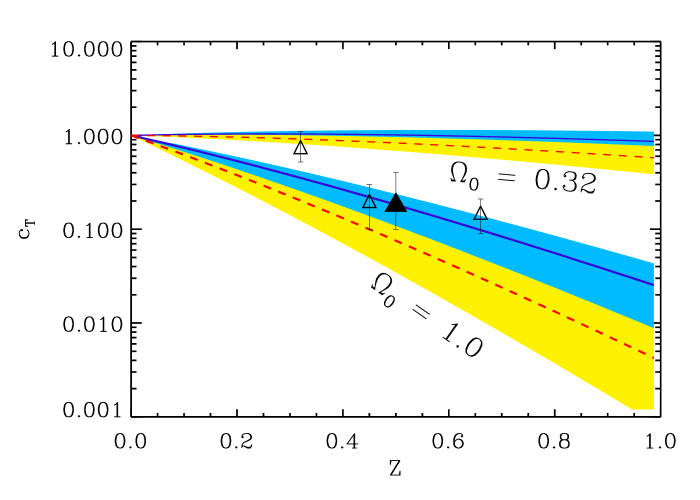
Figure 2: Relative evolution of the abundance of clusters above a given temperature. The continuous and dashed lines show the cluster abundance evolution for $T>4$ keV and $T>6$ keV, respectively The grey area delimits our estimate of the modeling uncertainty, taken from Oukbir & Blanchard (1997) and Oukbir et al. (1997). The triangles are from the observations as given by Carlberg al. (1997) and Bahcall et al. (1997). The point at $z=0.66$ is derived from the luminosity function of the EMSS. The open triangles correspond to clusters with $T>6$ keV, while the filled triangle is for $T>4$ keV, assuming no evolution in the $L_{x}-T_{x}$ relation.

The abundance of X-ray clusters at redshift 0.66 can be estimated from the EMSS (Luppino and Gioia 1995):

$$N(L_{[0.3-3.5]}>5.10^{44})\approx 1.10^{-8}$$ (6)

In the absence of evolution in the $L_{x}-T_{x}$ relation , such clusters would have temperatures greater than $5$ keV (Arnaud and Evrard 1997). The abundance of clusters deduced from the temperature distribution function at $z=0$ is, rather surprisingly, highly uncertain (see, for instance, Table 1 in Carlberg et al., 1997). To lower this uncertainty, we estimate the present–day abundance of similar clusters from the BCS luminosity function, which is constructed from a much larger cluster sample, (Ebeling et al., 1997). In the ROSAT band - $[0.1,2.4]\;$ keV - 4 to 6 keV clusters have a luminosity greater than $4.10^{44}{\rm erg/s/cm^{2}}$, yielding $N(>L)\sim 0.6\;10^{-7}$, giving:

$$\frac{n_{T}(z=0.66)}{n_{T}(z=0.00)}\approx 0.16\pm 0.06$$ (7)

which is direct and clean evidence for some kind of evolution. The above density will serve as our reference for the abundance at $z=0$ for the CNOC clusters: $c_{T}({\overline{z}}=0.27)\approx 0.44^{+0.29}_{-0.15}$ and $c_{T}({\overline{z}}=0.45)\approx 0.11^{+0.075}_{-0.045}$.

As we have already mentioned, open models ($\Omega\sim 0.2$), for which the temperature distribution function shows little evolution, cannot be consistent with the EMSS distribution unless there is strong negative evolution of the luminosity-temperature relation: whatever the value of $\Omega_{0}$, the properties of the cluster population (either the number density or the luminosity–temperature relation) must evolve in order to explain the EMSS redshift distribution. One may wonder whether a bias in the EMSS sample could lead to a severe underestimation of the cluster abundance at large $z$. This seems rather unlikely, for at such redshifts clusters are almost point–like compared to the size of the detection cell (5’); furthermore, no systematic bias has been found in the photometry (Nichol et al., 1997).

These numbers already give interesting insight concerning the density parameter of the universe. It is clear from Fig. 2 that the critical model is favored over a low–density model, according to the cluster abundances reported in the recent literature; however, a note of caution: it must be remembered that in all cases, the data were analyzed assuming, either implicitly or explicitly, a non–evolving relation between temperature and luminosity. It is for this same reason that our present conclusions are exactly the same as those given by Oukbir and Blanchard (1997): under the assumption of a non-evolving temperature-luminosity relation, the EMSS redshift distribution of X-ray clusters favors a high density universe. This result is supported by the additional information that available data on distant X-ray clusters does not demonstrate any sign of the strong negative evolution of the luminosity–temperature relation needed to save the open model (Sadat et al., 1998) (this is independent of the possible addition of a cosmological constant). This additional piece of information is critical to the conclusion, because without it, we have no way of understanding the flux limited selection of the EMSS in terms of temperature.

4 Conclusion and discussion

The purpose of this letter was to clarify the nature of the evolution of the cluster temperature distribution function. As we have seen, this evolution depends primarly on the amplitude of the fluctuations on the scale under consideration, $\sigma(M)$, and the cosmological background, $\Omega_{0}$. This is the origin of the robustness of the cosmological test initially proposed by Oukbir and Blanchard (1992). The EMSS redshift distribution, as modeled by Oukbir and Blanchard (1997), combined with the absence of observed negative evolution in the temperature–luminosity relation provided the first evidence for a high density universe from this technique (Sadat et al 1998). Our analysis leads to a similarly high value for the density of the universe. During the submission of this letter, we learned that similar conclusions were reached by two other groups who included ROSAT cluster redshift distributions (Borgani et al., 1998; Reichart et al, 1998). Because this test is primary sensitive to the dynamical behavior of the universe as a whole (through the growth rate of linear density fluctuations), we consider this to be the strongest evidence in favor of a critical density universe presently available.

- (1) Arnaud, M., Evrard, A.E. 1998, in preparation.
- (2) Bahcall, N.A., Fan, X., Cen, R. 1997, ApJ, 485, L53
- (3) Barbosa D., Bartlett J.G., Blanchard A., Oukbir, J. 1996, A&A, 314, 13
- (4) Bartlett, J.G. 1997, Proceedings of the 1st Moroccan School of Astrophysics, ed. D. Valls-Gabaud et al., A.S.P. Conf. Ser., vol. 126, p. 365
- (5) Borgani, S., Rosati, P., Tozzi, P., Norman, C. 1998, ApJ, submitted.
- (6) Carlberg, R.G., Morris, S.L., Yee, H.K.C., Ellingson, E. 1997, ApJ, 479, L19
- (7) Colafrancesco, S., Mazzotta, P., Vittorio, N. 1997, ApJ, 488, 566
- (8) Ebeling, H., Edge, A.C., Fabian, A.C., Allen, S.W., Crawford, C.S. 1997, ApJL, 479, L101
- (9) Evrard, A.E., Metzler, C.A., Navarro, J.F. 1996, ApJ, 469, 494
- (10) Fan, X., Bahcall, N.A., Cen, R. 1997, ApJ, 490, L123
- (11) Gioia, I.M., Luppino, G.A. 1994, ApJS, 94, 583
- (12) Henry, J.P, Arnaud, K.A. 1991, ApJ, 372, 410
- (13) Henry, J.P. 1997, ApJ, 489, L1
- (14) Lacey, C., Cole S. 1994, MNRAS 271, 676
- (15) Luppino, G.A., Gioia, I.M. 1995, ApJ, 445, L77
- (16) Nichol, R.C., Holden, B.P., Romer, A.K., Ulmer, M.P., Burke, D.J., Collins, C.A. 1997, ApJ., 481, 644
- (17) Oukbir, J., Blanchard A. 1992, A&A, 262, L21
- (18) Oukbir, J., Blanchard A. 1997, A&A, 317, 10
- (19) Oukbir, J., Bartlett, J.G., Blanchard, A. 1997, A&A, 320, 365
- (20) Press W.H., Schechter, P. 1974, ApJ, 187, 425
- (21) Reichart et al, 1998, astro-ph/9802153
- (22) Sadat, R., Blanchard, A., Oukbir, J. 1998, A&A, 329, 21
- (23) Viana, P.T.R., Liddle, A.R. 1996, MNRAS, 281, 323