Radio galaxies and structure formation To appear in proceedings of the KNAW colloquium
The most distant radio galaxies, Amsterdam, October 1997

Abstract

This review discusses three ways in which radio galaxies and other high-redshift objects can give us information on the nature and statistics of cosmological inhomogeneities, and how they have evolved between high redshift and the present: (1) The present-day spatial distribution and clustering of radio galaxies; (2) The evolution of radio-galaxy clustering and biased clustering at high redshift; (3) Measuring density perturbation spectra from the abundances of high-redshift galaxies.

Royal Observatory, Blackford Hill, Edinburgh EH9 3HJ, UK

1 Present-day clustering of radio galaxies

Radio galaxies are interesting probes of large-scale structure in the universe, and give a view of the galaxy distribution which differs significantly from that obtained in other wavebands. Radio selection is uniform over the sky and independent of galactic extinction, so that reliably complete catalogues can be obtained over large areas. As a result, the apparent uniformity of the distribution of radio sources in early surveys such as 4C and Parkes gave the first convincing evidence for the large-scale homogeneity of the Universe (Webster 1977). This uniformity arises because even relatively bright samples of radio galaxies are at redshifts $z\simeq 1$, so that projection effects give a huge dilution of any intrinsic spatial clustering. The 3D clustering of radio galaxies was first detected by Peacock & Nicholson (1991; PN91), using a redshift survey of 329 galaxies with $z<0.1$ and $S({\rm 1.4~{}GHz})\mathrel{\lower 2.58334pt\hbox{$\buildrel{\textstyle>}\over{\scriptstyle\sim}$}}500~{}{\rm mJy}$. The result was a correlation function measured in redshift space of

$$\xi_{rg}(s)=[s/11\,h^{-1}\,{\rm Mpc}]^{-1.8}$$ (1)

($h\equiv H_{0}/100\;{\rm km\,s^{-1}\,Mpc^{-1}}$). This corresponds to a clustering amplitude intermediate between normal galaxies and rich clusters of galaxies, as seems appropriate give that radio galaxies are normally found in moderately rich groups (e.g. Allington-Smith et al. 1993).

Figure 1: One of the 6 slices of the Las Campanas Redshift Survey, containing 4706 galaxies brighter than about $R=17.5$, together with the 138 galaxies detected in the NVSS to a flux limit of 2.5 mJy at 1.4 GHz. It is clear that the radio galaxies trace out very much the same large-scale network of filaments and voids, albeit in a more dilute fashion.

However, redshift surveys move on rapidly: in the region of $10^{5}$ galaxy redshifts are now known, and it should be possible to do very much better than PN91 today. Particularly, the PN91 survey has a very low density owing to its relatively bright flux limit; in order to see how radio galaxies follow the pattern of LSS in detail, deeper surveys are needed. Rather than attempt to construct a completely new radio-selected redshift survey, it is most efficient to match large optically-selected redshift surveys with the new deep all-sky radio databases such as the NVSS and FIRST. The largest complete redshift survey for which this exercise is possible is the Las Campanas Redshift Survey (Shectman et al. 1996), which contains 26,418 galaxies to $R\simeq 17.5$. The LCRS contains six slices approximately $1.5^{\circ}\times 60^{\circ}$, of which four are at sufficiently high declination to overlap with the NVSS survey (Condon et al. 1997), which has a flux limit of about 2.5 mJy at 1.4 GHz. Matching these two catalogues with a positional tolerance of 20 arcsec yields a total of 451 radio-selected galaxies. This significantly exceeds the PN91 sample in size, although the relatively modest detection rate shows that much larger parent redshift surveys such as Sloan and 2dF will be needed to push radio-selected redshift surveys into the $N=10^{4}$ – $10^{5}$ regime. In the meantime, it is interesting to compare the clustering in this new sample with that of PN91.

It is common to use the homogeneous distance-redshift relation to deduce radii, and hence 3D coordinates for galaxies in redshift surveys. From these, it is natural to evaluate the spatial two-point correlation function $\xi(r)$ as a measure of clustering in the universe. However, in practice the radii are affected by large-scale coherent velocities, small-scale virialized motions and redshift errors. A better statistic, which is independent of all these effects, is the projected correlation function:

$$\Xi(r)=\int_{-\infty}^{\infty}\xi[(r^{2}+x^{2})^{1/2}]\;dx.$$ (2)

Fig. 2 shows the result for $\Xi(r)$ measured from the sample of 451 NVSS/LCRS galaxies. The plot shows both the raw data, together with power-law models:

$$\xi(r)=(r/r_{0})^{-\gamma}.$$ (3)

The canonical numbers for blue-selected radio-quiet galaxies are $r_{0}=5\,h^{-1}\,{\rm Mpc}$ and $\gamma=1.8$. The radio-loud result in this sample is approximately $6.5\,h^{-1}\,{\rm Mpc}$: the radio-loud subset of the LCRS is clustered only slightly more strongly than the whole LCRS – in apparent conflict with PN91. The larger PN91 result of $11\,h^{-1}\,{\rm Mpc}$ was based on the redshift-space $\xi(s)$, which will tend to give a boosted value of $r_{0}$. In the linear analysis of Kaiser (1987), this increases $\xi$ by a factor

$$\xi\rightarrow\xi\;[1+2\beta/3+\beta^{2}/5],$$ (4)

where $\beta=\Omega^{0.6}/b$ and $b$ is the bias parameter. The relative bias between PN91 and blue-selected galaxies gives $\beta_{\rm opt}/\beta_{\rm rad}\simeq 1.9$ (see Peacock & Dodds 1994). Since $\beta_{\rm opt}$ is currently thought to lie close to 0.5 (Hamilton 1997), this suggests a boost factor of 1.2, and a real-space $r_{0}\simeq 10\,h^{-1}\,{\rm Mpc}$ for the PN91 sample. This is larger than the NVSS/LCRS result, but it is not clear that there is any inconsistency: although the typical redshifts of the two samples are similar, their radio flux-density limits differ by about a factor of 200. The PN91 radio galaxies are luminous AGN, whereas many of the NVSS/LCRS galaxies will be starburst galaxies similar to those found in the IRAS surveys. Starbursts obey the approximate rule $S_{\rm 60\mu m}=90S_{\rm 1.4~{}GHz}$, so that the NVSS galaxies should be comparable in flux to the IRAS FSS limit of 0.25 Jy (Rowan-Robinson et al. 1994). Since IRAS galaxies are well known to cluster even less strongly than optical galaxies, the modest value of $r_{0}$ is not a surprise. Independent confirmation of the PN91 result for ‘proper’ radio galaxies will require a new radio-selected redshift survey at brighter flux densities.

Figure 2: The real-space projected correlation function, $\Xi(r)$, for the NVSS galaxies in the four LCRS slices for which the two surveys overlap. The error bars indicate Poissonian errors based on the observed pair counts, and evidently these are an underestimate of the true error in the intermediate regime, $r\simeq 3\,h^{-1}\,{\rm Mpc}$. The dashed line shows the normal fit to optical galaxy clustering: $\xi=[r/r_{0}]^{-\gamma}$, with $\gamma=1.8$ and $r_{0}=5\,h^{-1}\,{\rm Mpc}$. The solid line shows the fit to the NVSS/LCRS sample, indicating a slightly larger scale-length of $6.5\,h^{-1}\,{\rm Mpc}$.

2 Evolution of clustering

It would be interesting to extend these studies to higher redshifts. This can be done without using a complete faint redshift survey, by using the angular clustering of a flux-limited survey. If the form of the redshift distribution is known, the projection effects can be disentangled in order to estimate the 3D clustering at the average redshift of the sample. For small angles, and where the redshift shell being studied is thicker than the scale of any clustering, the spatial and angular correlation functions are related by Limber’s equation (e.g. Peebles 1980):

$$w(\theta)=\int_{0}^{\infty}y^{4}\phi^{2}F^{2}(y)\,dy\ \int_{-\infty}^{\infty}\xi(\sqrt{x^{2}+y^{2}\theta^{2}})\;dx,$$ (5)

where $y$ is dimensionless comoving distance (transverse part of the FRW metric is $[R(t)y\,d\theta]^{2}$), and $F(y)=[1-ky^{2}]^{-1/2}$; the selection function for radius $y$ is normalized so that $\int y^{2}\phi(y)F(y)\;dy=1$.

Until recently, this equation was of somewhat academic interest for radio astronomers, since there were no reliable detections of angular clustering. This has changed with the FIRST survey, which has measured $w(\theta)$ to high precision for a limit of 1 mJy at 1.4 GHz (Cress et al. 1996). Their result detects clustering at separations between 0.02 and 2 degrees, and is fitted by a power law:

$$w(\theta)=0.003\,[\theta/{\rm degrees}]^{-1.1}.$$ (6)

There had been earlier claims of detections of angular clustering, notably the 87GB survey (Loan, Lahav & Wall 1996), but these were of only bare significance (although, in retrospect, the level of clustering in 87GB is consistent with the FIRST measurement).

Limber’s equation requires the redshift-dependent correlation function, and this is commonly parameterized as follows:

$$\xi(r,z)=[r/r_{0}]^{-\gamma}\,(1+z)^{-(3-\gamma+\epsilon)},$$ (7)

where $\epsilon=0$ is stable clustering; $\epsilon=\gamma-3$ is constant comoving clustering; $\epsilon=\gamma-1$ is $\Omega=1$ linear-theory evolution. Peacock (1997) showed that the expected evolution in the quasilinear regime ($\xi\sim 1$ – 100) is significantly more rapid: up to $\epsilon\simeq 3$.

Discussion of the 87GB and FIRST results in terms of Limber’s equation has tended to focus on values of $\epsilon$ in the region of 0. Cress et al. (1996) concluded that the $w(\theta)$ results were consistent with the PN91 value of $r_{0}\simeq 10\,h^{-1}\,{\rm Mpc}$ (although they were not very specific about $\epsilon)$. Loan et al. (1996) measured $w(1^{\circ})\simeq 0.005$ for a 5-GHz limit of 50 mJy, and inferred $r_{0}\simeq 12\,h^{-1}\,{\rm Mpc}$ for $\epsilon=0$, falling to $r_{0}\simeq 9\,h^{-1}\,{\rm Mpc}$ for $\epsilon=-1$. If we take the NVSS/LCRS value of the local clustering for radio sources, $r_{0}\simeq 6.5\,h^{-1}\,{\rm Mpc}$, then the observed angular clustering in fact requires $\epsilon$ in the region of $-1.5$ or smaller: in other words, little or no evolution of $\xi$ with redshift.

Indeed, this conclusion can be reached in a rather less model-dependent fashion. The reason there is a strong degeneracy between $r_{0}$ and $\epsilon$ is that $r_{0}$ parameterizes the $z=0$ clustering, whereas the observations refer to a typical redshift of around unity. This means that $\xi(z=1)$ can be inferred quite robustly, without much dependence on the rate of evolution. Since the strength of clustering for optical galaxies at $z=1$ is known to correspond to the much smaller number of $r_{0}\simeq 2\,h^{-1}\,{\rm Mpc}$ (e.g. Le Fèvre et al. 1996), we see that radio galaxies at this redshift have a relative bias parameter of close to 3. This tendency for the relative bias to increase with redshift probably arises partly because the high-redshift sample members will be more powerful radio galaxies, but also is likely to be related to the rareness of such massive host galaxies at early times.

3 Formation of high-redshift galaxies

The challenge now is to ask how these results can be understood in current models for cosmological structure formation. It is widely believed that the sequence of cosmological structure formation was hierarchical, originating in a density power spectrum with increasing fluctuations on small scales. The large-wavelength portion of this spectrum is accessible to observation today through studies of galaxy clustering in the linear and quasilinear regimes. However, nonlinear evolution has effectively erased any information on the initial spectrum for wavelengths below about 1 Mpc. The most sensitive way of measuring the spectrum on smaller scales is via the abundances of high-redshift objects; the amplitude of fluctuations on scales of individual galaxies governs the redshift at which these objects first undergo gravitational collapse. The small-scale amplitude also influences clustering, since rare early-forming objects are strongly correlated, as first realized by Kaiser (1984).

It will be especially interesting to apply these arguments about the small-scale spectrum to a class of very early-forming galaxies discussed at this meeting by Dunlop. These are the red optical identifications of 1-mJy radio galaxies, for which deep absorption-line spectroscopy has proved that the red colours result from a well-evolved stellar population, with a minimum stellar age of 3.5 Gyr for 53W091 at $z=1.55$ (Dunlop et al. 1996; Spinrad et al. 1997), and 4.0 Gyr for 53W069 at $z=1.43$ (Dey et al. 1998). Such ages push the formation era for these galaxies back to extremely high redshifts, and it is of interest to ask what level of small-scale power is needed in order to allow this early formation.

3.1 Press-Schechter apparatus

The standard framework for interpreting the abundances of high-redshift objects in terms of structure-formation models, was outlined by Efstathiou & Rees (1988). The formalism of Press & Schechter (1974) gives a way of calculating the fraction $F_{c}$ of the mass in the universe which has collapsed into objects more massive than some limit $M$:

$$F_{c}(>M,z)=1-{\rm erf}\,\left[{\delta_{c}\over\sqrt{2}\,\sigma(M)}\right].$$ (8)

Here, $\sigma(M)$ is the rms fractional density contrast obtained by filtering the linear-theory density field on the required scale. In practice, this filtering is usually performed with a spherical ‘top hat’ filter of radius $R$, with a corresponding mass of $4\pi\rho_{b}R^{3}/3$, where $\rho_{b}$ is the background density. The number $\delta_{c}$ is the linear-theory critical overdensity, which for a ‘top-hat’ overdensity undergoing spherical collapse is $1.686$ – virtually independent of $\Omega$. This form describes numerical simulations very well (see e.g. Ma & Bertschinger 1994). The main assumption is that the density field obeys Gaussian statistics, which is true in most inflationary models. Given some estimate of $F_{c}$, the number $\sigma(R)$ can then be inferred. Note that for rare objects this is a pleasingly robust process: a large error in $F_{c}$ will give only a small error in $\sigma(R)$, because the abundance is exponentially sensitive to $\sigma$.

Total masses are of course ill-defined, and a better quantity to use is the velocity dispersion. Virial equilibrium for a halo of mass $M$ and proper radius $r$ demands a circular orbital velocity of

$$V_{c}^{2}={GM\over r}$$ (9)

For a spherically collapsed object this velocity can be converted directly into a Lagrangian comoving radius which contains the mass of the object within the virialization radius (e.g. White, Efstathiou & Frenk 1993):

$$R/\,h^{-1}\,{\rm Mpc}={2^{1/2}[V_{c}/100\;{\rm km\,s^{-1}}]\over\Omega_{m}^{1/2}(1+z_{c})^{1/2}f_{c}^{1/6}}.$$ (10)

Here, $z_{c}$ is the redshift of virialization; $\Omega_{m}$ is the present value of the matter density parameter; $f_{c}$ is the density contrast at virialization of the newly-collapsed object relative to the background, which is adequately approximated by

$$f_{c}=178/\Omega_{m}^{0.6}(z_{c}),$$ (11)

with only a slight sensitivity to whether $\Lambda$ is non-zero (Eke, Cole & Frenk 1996).

For isothermal-sphere haloes, the velocity dispersion is

$$\sigma_{v}=V_{c}/\sqrt{2}.$$ (12)

Given a formation redshift of interest, and a velocity dispersion, there is then a direct route to the Lagrangian radius from which the proto-object collapsed.

3.2 Abundances and masses of high-redshift objects

In addition to the red mJy galaxies, two classes of high-redshift object have been used recently to set constraints on the small-scale power spectrum at high redshift:

(1) Damped Lyman-$\alpha$ systems  Damped Lyman-$\alpha$ absorbers are systems with HI column densities greater than $\sim 2\times 10^{24}\;\rm m^{-2}$ (Lanzetta et al. 1991). If the fraction of baryons in the virialized dark matter halos equals the global value $\Omega_{\scriptscriptstyle\rm B}$, then data on these systems can be used to infer the total fraction of matter that has collapsed into bound structures at high redshifts (Ma & Bertschinger 1994, Mo & Miralda-Escudé 1994; Kauffmann & Charlot 1994; Klypin et al. 1995). The highest measurement at $\langle z\rangle\simeq 3.2$ implies $\Omega_{\scriptscriptstyle\rm HI}\simeq 0.0025h^{-1}$ (Lanzetta et al. 1991; Storrie-Lombardi, McMahon & Irwin 1996). If $\Omega_{\scriptscriptstyle\rm B}h^{2}=0.02$ is adopted, as a compromise between the lower Walker et al. (1991) nucleosynthesis estimate and the more recent estimate of 0.025 from Tytler et al. (1996), then

$$F_{c}={\Omega_{\scriptscriptstyle\rm HI}\over\Omega_{\scriptscriptstyle\rm B}}\simeq 0.12h$$ (13)

for these systems. In this case alone, an explicit value of $h$ is required in order to obtain the collapsed fraction; $h=0.65$ is assumed.

The photoionizing background prevents virialized gaseous systems with circular velocities of less than about $50\;{\rm km\,s^{-1}}$ from cooling efficiently, so that they cannot contract to the high density contrasts characteristic of galaxies (e.g. Efstathiou 1992). Mo & Miralda-Escudé (1994) used the circular velocity range 50 – $100\;{\rm km\,s^{-1}}$ ($\sigma_{v}=35$ – $70\;{\rm km\,s^{-1}}$) to model the damped Lyman alpha systems. Reinforcing the photoionization argument, detailed hydrodynamic simulations imply that the absorbers are not expected to be associated with very massive dark-matter haloes (Haehnelt, Steinmetz & Rauch 1997). This assumption is consistent with the rather low luminosity galaxies detected in association with the absorbers in a number of cases (Le Brun et al. 1996).

(2) Lyman-limit galaxies  Steidel et al. (1996) identified star-forming galaxies between $z=3$ and 3.5 by looking for objects with a spectral break redwards of the $U$ band. The treatment of these Lyman-limit galaxies in this paper is similar to that of Mo & Fukugita (1996), who compared the abundances of these objects to predictions from various models. Steidel et al. give the comoving density of their galaxies as

$$N(\Omega=1)\simeq 10^{-2.54}\;(\,h^{-1}\,{\rm Mpc})^{-3}.$$ (14)

This is a high number density, comparable to that of $L^{*}$ galaxies in the present Universe. The mass of $L^{*}$ galaxies corresponds to collapse of a Lagrangian region of volume $\sim 1\,\rm Mpc^{3}$, so the collapsed fraction would be a few tenths of a per cent if the Lyman-limit galaxies had similar masses.

Direct dynamical determinations of these masses are still lacking in most cases. Steidel et al. attempt to infer a velocity width by looking at the equivalent width of the C and Si absorption lines. These are saturated lines, and so the equivalent width is sensitive to the velocity dispersion; values in the range

$$\sigma_{v}\simeq 180-320\;{\rm km\,s^{-1}}$$ (15)

are implied. These numbers may measure velocities which are not due to bound material, in which case they would give an upper limit to $V_{c}/\sqrt{2}$ for the dark halo. A more recent measurement of the velocity width of the H$\alpha$ emission line in one of these objects gives a dispersion of closer to $100\;{\rm km\,s^{-1}}$ (Pettini, private communication), consistent with the median velocity width for Ly$\alpha$ of $140\;{\rm km\,s^{-1}}$ measured in similar galaxies in the HDF (Lowenthal et al. 1997). Of course, these figures could underestimate the total velocity dispersion, since they are dominated by emission from the central regions only. For the present, the range of values $\sigma_{v}=100$ to $320\;{\rm km\,s^{-1}}$ will be adopted, and the sensitivity to the assumed velocity will be indicated. In practice, this uncertainty in the velocity does not produce an important uncertainty in the conclusions.

(3) Red radio galaxies  Two extremely red galaxies were found at $z=1.43$ and 1.55, over an area $1.68\times 10^{-3}\;\rm sr$, so a minimal comoving density is from one galaxy in this redshift range:

$$N(\Omega=1)\mathrel{\lower 2.58334pt\hbox{$\buildrel{\textstyle>}\over{\scriptstyle\sim}$}}10^{-5.87}\;(\,h^{-1}\,{\rm Mpc})^{-3}.$$ (16)

This figure is comparable to the density of the richest Abell clusters, and is thus in reasonable agreement with the discovery that rich high-redshift clusters appear to contain radio-quiet examples of similarly red galaxies (Dickinson 1995).

Since the velocity dispersions of these galaxies are not observed, they must be inferred indirectly. This is possible because of the known present-day Faber-Jackson relation for ellipticals. For 53W091, the large-aperture absolute magnitude is

$$M_{V}(z=1.55\mid\Omega=1)\simeq-21.62-5\log_{10}h$$ (17)

(measured direct in the rest frame). According to Solar-metallicity spectral synthesis models, this would be expected to fade by about 0.9 mag. between $z=1.55$ and the present, for an $\Omega=1$ model of present age 14 Gyr (note that Bender et al. 1996 have observed a shift in the zero-point of the $M-\sigma_{v}$ relation out to $z=0.37$ of a consistent size). If we compare these numbers with the $\sigma_{v}$ – $M_{V}$ relation for Coma ($m-M=34.3$ for $h=1$) taken from Dressler (1984), this predicts velocity dispersions in the range

$$\sigma_{v}=222\;{\rm to}\;292\;\;{\rm km\,s^{-1}}.$$ (18)

This is a very reasonable range for a giant elliptical, and it adopted in the following analysis.

Having established an abundance and an equivalent circular velocity for these galaxies, the treatment of them will differ in one critical way from the Lyman-$\alpha$ and Lyman-limit galaxies. For these, the normal Press-Schechter approach assumes the systems under study to be newly born. For the Lyman-$\alpha$ and Lyman-limit galaxies, this may not be a bad approximation, since they are evolving rapidly and/or display high levels of star-formation activity. For the radio galaxies, conversely, their inactivity suggests that they may have existed as discrete systems at redshifts much higher than $z\simeq 1.5$. The strategy will therefore be to apply the Press-Schechter machinery at some unknown formation redshift, and see what range of redshift gives a consistent degree of inhomogeneity.

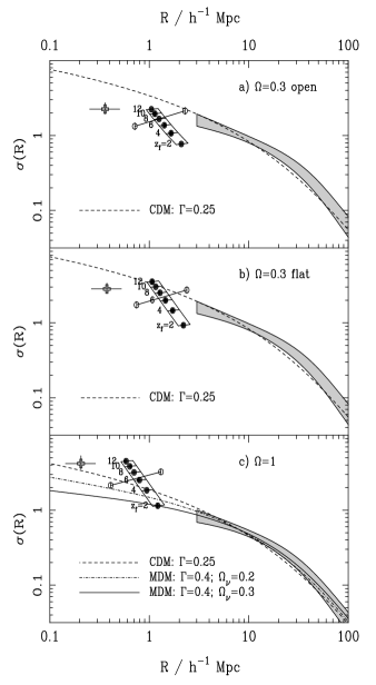
Figure 3: The present-day linear fractional rms fluctuation in density averaged in spheres of radius $R$. The data points are Lyman-$\alpha$ galaxies (open cross) and Lyman-limit galaxies (open circles) The diagonal band with solid points shows red radio galaxies with assumed collapse redshifts 2, 4, …12. The vertical error bars show the effect of a change in abundance by a factor 2. The horizontal errors correspond to different choices for the circular velocities of the dark-matter haloes that host the galaxies. The shaded region at large $R$ gives the results inferred from galaxy clustering. The lines show CDM and MDM predictions, with a large-scale normalization of $\sigma_{8}=0.55$ for $\Omega=1$ or $\sigma_{8}=1$ for the low-density models.

4 The small-scale fluctuation spectrum

4.1 The empirical spectrum

Fig. 3 shows the $\sigma(R)$ data which result from the Press-Schechter analysis, for three cosmologies. The $\sigma(R)$ numbers measured at various high redshifts have been translated to $z=0$ using the appropriate linear growth law for density perturbations.

The open symbols give the results for the Lyman-limit (largest $R$) and Lyman-$\alpha$ (smallest $R$) systems. The approximately horizontal error bars show the effect of the quoted range of velocity dispersions for a fixed abundance; the vertical errors show the effect of changing the abundance by a factor 2 at fixed velocity dispersion. The locus implied by the red radio galaxies sits in between. The different points show the effects of varying collapse redshift: $z_{c}=2,4,\dots,12$ [lowest redshift gives lowest $\sigma(R)$]. Clearly, collapse redshifts of 6 – 8 are favoured for consistency with the other data on high-redshift galaxies, independent of theoretical preconceptions and independent of the age of these galaxies. This level of power ($\sigma[R]\simeq 2$ for $R\simeq 1\,h^{-1}\,{\rm Mpc}$) is also in very close agreement with the level of power required to produce the observed structure in the Lyman alpha forest (Croft et al. 1997), so there is a good case to be made that the fluctuation spectrum has now been measured in a consistent fashion down to below $R\simeq 1\,h^{-1}\,{\rm Mpc}$.

The shaded region at larger $R$ shows the results deduced from clustering data (Peacock 1997). It is clear an $\Omega=1$ universe requires the power spectrum at small scales to be higher than would be expected on the basis of an extrapolation from the large-scale spectrum. Depending on assumptions about the scale-dependence of bias, such a ‘feature’ in the linear spectrum may also be required in order to satisfy the small-scale present-day nonlinear galaxy clustering (Peacock 1997). Conversely, for low-density models, the empirical small-scale spectrum appears to match reasonably smoothly onto the large-scale data.

Fig. 3 also compares the empirical data with various physical power spectra. A CDM model (using the transfer function of Bardeen et al. 1986) with shape parameter $\Gamma=\Omega h=0.25$ is shown as a reference for all models. This has approximately the correct level of small-scale power, but significantly over-predicts intermediate-scale clustering, as discussed in Peacock (1997). The empirical LSS shape is better described by MDM with $\Omega h\simeq 0.4$ and $\Omega_{\nu}\simeq 0.3$. This is the lowest curve in Fig. 1c, reproduced from the fitting formula of Pogosyan & Starobinsky (1995; see also Ma 1996). However, this curve fails to supply the required small-scale power, by about a factor 3 in $\sigma$; lowering $\Omega_{\nu}$ to 0.2 still leaves a very large discrepancy. This conclusion is in agreement with e.g. Mo & Miralda-Escudé (1994), Ma & Bertschinger (1994), but conflicts slightly with Klypin et al. (1995), who claimed that the $\Omega_{\nu}=0.2$ model was acceptable. This difference arises partly because Klypin et al. adopt a lower value for $\delta_{c}$ (1.33 as against 1.686 here), and also because they adopt the high normalization of $\sigma_{8}=0.7$; the net effect of these changes is to boost the model relative to the small-scale data by a factor of 1.6, which would allow marginal consistency for the $\Omega_{\nu}=0.2$ model. MDM models do allow a higher normalization than the conventional figure of $\sigma_{8}=0.55$, partly because of the very flat small-scale spectrum, and also because of the effects of random neutrino velocities. However, such shifts are at the 10 per cent level (Borgani et al. 1997a, 1997b), and $\sigma_{8}=0.7$ would probably still give a cluster abundance in excess of observation. The consensus of more recent modelling is that even $\Omega_{\nu}=0.2$ MDM is deficient in small-scale power (Ma et al. 1997; Gardner et al. 1997).

All the models in Fig. 1 assume $n=1$; in fact, consistency with the COBE results for this choice of $\sigma_{8}$ and $\Omega h$ requires a significant tilt for flat CDM models, $n\simeq 0.9$ (whereas open CDM models require $n$ substantially above unity). Over the range of scales probed by LSS, changes in $n$ are largely degenerate with changes in $\Omega h$, but the small-scale power is more sensitive to tilt than to $\Omega h$. Tilting the $\Omega=1$ models is not attractive, since it increases the tendency for model predictions to lie below the data. However, a tilted low-$\Omega$ flat CDM model would agree moderately well with the data on all scales, with the exception of the ‘bump’ around $R\simeq 30\,h^{-1}\,{\rm Mpc}$. Testing the reality of this feature will therefore be an important task for future generations of redshift survey.

4.2 Collapse redshifts and ages

Are the collapse redshifts inferred above consistent with the age data on the red radio galaxies? First bear in mind that in a hierarchy some of the stars in a galaxy will inevitably form in sub-units before the epoch of collapse. At the time of final collapse, the typical stellar age will be some fraction $\alpha$ of the age of the universe at that time:

$${\rm age}=t(z_{\rm obs})-t(z_{c})+\alpha t(z_{c}).$$ (19)

We can rule out $\alpha=1$ (i.e. all stars forming in small subunits just after the big bang). For present-day ellipticals, the tight colour-magnitude relation only allows an approximate doubling of the mass through mergers since the termination of star formation (Bower at al. 1992). This corresponds to $\alpha\simeq 0.3$ (Peacock 1991). A non-zero $\alpha$ just corresponds to scaling the collapse redshift as

$${\rm apparent}\ (1+z_{c})\propto(1-\alpha)^{-2/3},$$ (20)

since $t\propto(1+z)^{-3/2}$ at high redshifts for all cosmologies. For example, a galaxy which collapsed at $z=6$ would have an apparent age corresponding to a collapse redshift of 7.9 for $\alpha=0.3$.

Converting the ages for the galaxies to an apparent collapse redshift depends on the cosmological model, but particularly on $H_{0}$. Some of this uncertainty may be circumvented by fixing the age of the universe. After all, it is of no interest to ask about formation redshifts in a model with e.g. $\Omega=1$, $h=0.7$ when the whole universe then has an age of only 9.5 Gyr. If $\Omega=1$ is to be tenable then either $h<0.5$ against all the evidence or there must be an error in the stellar evolution timescale. If the stellar timescales are wrong by a fixed factor, then these two possibilities are degenerate. It therefore makes sense to measure galaxy ages only in units of the age of the universe – or, equivalently, to choose freely an apparent Hubble constant which gives the universe an age comparable to that inferred for globular clusters. In this spirit, Fig. 4 gives apparent ages as a function of effective collapse redshift for models in which the age of the universe is forced to be 14 Gyr (e.g. Jimenez et al. 1996).

Figure 4: The age of a galaxy at $z=1.5$, as a function of its collapse redshift (assuming an instantaneous burst of star formation). The various lines show $\Omega=1$ [solid]; open $\Omega=0.3$ [dotted]; flat $\Omega=0.3$ [dashed]. In all cases, the present age of the universe is forced to be 14 Gyr.

This plot shows that the ages of the red radio galaxies are not permitted very much freedom. Formation redshifts in the range 6 to 8 predict an age of close to 3.0 Gyr for $\Omega=1$, or 3.7 Gyr for low-density models, irrespective of whether $\Lambda$ is nonzero. The age-$z_{c}$ relation is rather flat, and this gives a robust estimate of age once we have some idea of $z_{c}$ through the abundance arguments. Conversely, it is almost impossible to determine the collapse redshift reliably from the spectral data, since a very high precision would be required both in the age of the galaxy and in the age of the universe.

What conclusions can then be reached about allowed cosmological models? If we take an apparent $z_{c}=8$ from the power-spectrum arguments, then the apparent minimum age of $>4$ Gyr for 53W069 can very nearly be satisfied in both low-density models (a current age of 14.5 Gyr would be required), but is unattainable for $\Omega=1$. In the high-density case, a current age of 17.6 Gyr would be required to attain the required age for $z_{c}=8$; this requires a Hubble constant of $h=0.38$. As argued above, this conclusion is highly insensitive to the assumed value of $z_{c}$. If the true value of $h$ does turn out to be close to 0.5, then it might be argued that $\Omega=1$ is consistent with the data, given realistic uncertainties. The ages for the low-density models would in this case be large by comparison with the observed radio-galaxy ages. However, the ages obtained by modelling spectra with a single burst can only be lower limits to the true age for the bulk of the stars; we could easily be observing an even older burst which is made bluer by a little recent star formation. A low $h$ measurement would therefore not rule out low-density models.

Figure 5: The bias parameter at $z=3.2$ predicted for the Lyman-limit galaxies, as a function of their assumed circular velocity. Dotted line shows $\Omega=0.3$ open; dashed line is $\Omega=0.3$ flat; solid line is $\Omega=1$. A substantial bias in the region of $b\simeq 6$ is predicted rather robustly.

5 Biased clustering at high redshifts

5.1 Predictions from the power spectrum

An interesting aspect of these results is that the level of power on 1-Mpc scales is only moderate: $\sigma(1\,h^{-1}\,{\rm Mpc})\simeq 2$. At $z\simeq 3$, the corresponding figure would have been much lower, making systems like the Lyman-limit galaxies rather rare. For Gaussian fluctuations, as assumed in the Press-Schechter analysis, such systems will be expected to display spatial correlations which are strongly biased with respect to the underlying mass. The linear bias parameter depends on the rareness of the fluctuation and the rms of the underlying field as

$$b=1+{\nu^{2}-1\over\nu\sigma}=1+{\nu^{2}-1\over\delta_{c}}$$ (21)

(Kaiser 1984; Cole & Kaiser 1989; Mo & White 1996), where $\nu=\delta_{c}/\sigma$, and $\sigma^{2}$ is the fractional mass variance at the redshift of interest.

In this analysis, $\delta_{c}=1.686$ is assumed. Variations in this number of order 10 per cent have been suggested by authors who have studied the fit of the Press-Schechter model to numerical data. These changes would merely scale $b-1$ by a small amount; the key parameter is $\nu$, which is set entirely by the collapsed fraction. For the Lyman-limit galaxies, typical values of this parameter are $\nu\simeq 3$, and it is clear that very substantial values of bias are expected, as illustrated in Figure 5.

This diagram shows how the predicted bias parameter varies with the assumed circular velocity, for a number density of galaxies fixed at the level observed by Steidel et al. (1996). The sensitivity to cosmological parameter is only moderate; at $V_{c}=200\;{\rm km\,s^{-1}}$, the predicted bias is $b\simeq 4.6$, 5.5, 5.8 for the open, flat and critical models respectively. These numbers scale approximately as $V_{c}^{-0.4}$, and $b$ is within 20 per cent of 6 for most plausible parameter combinations. Strictly, the bias values determined here are upper limits, since the numbers of collapsed haloes of this circular velocity could in principle greatly exceed the numbers of observed Lyman-limit galaxies. However, the undercounting would have to be substantial: increasing the collapsed fraction by a factor 10 reduces the implied bias by a factor of about 1.5. A substantial bias seems difficult to avoid, as has been pointed out in the context of CDM models by Baugh, Cole & Frenk (1997).

5.2 Clustering of Lyman-limit galaxies

These calculations are relevant to the recent detection by Steidel et al. (1997) of strong clustering in the population of Lyman-limit galaxies at $z\simeq 3$. The evidence takes the form of a redshift histogram binned at $\Delta z=0.04$ resolution over a field $8.7^{\prime}\times 17.6^{\prime}$ in extent. For $\Omega=1$ and $z=3$, this probes the density field using a cell with dimensions

$${\rm cell}=15.4\times 7.6\times 15.0\;[\,h^{-1}\,{\rm Mpc}]^{3}.$$ (22)

Conveniently, this has a volume equivalent to a sphere of radius $7.5\,h^{-1}\,{\rm Mpc}$, so it is easy to measure the bias directly by reference to the known value of $\sigma_{8}$. Since the degree of bias is large, redshift-space distortions from coherent infall are small; the cell is also large enough that the distortions of small-scale random velocities at the few hundred $\;{\rm km\,s^{-1}}$ level are also small. Using the model of equation (11) of Peacock (1997) for the anisotropic redshift-space power spectrum and integrating over the exact anisotropic window function, the above simple volume argument is found to be accurate to a few per cent for reasonable power spectra:

$$\sigma_{\rm cell}\simeq b(z=3)\;\sigma_{7.5}(z=3),$$ (23)

defining the bias factor at this scale. The results of Mo & White (1996) suggest that the scale-dependence of bias should be weak.

In order to estimate $\sigma_{\rm cell}$, simulations of synthetic redshift histograms were made, using the method of Poisson-sampled lognormal realizations described by Broadhurst, Taylor & Peacock (1995): using a $\chi^{2}$ statistic to quantify the nonuniformity of the redshift histogram, it appears that $\sigma_{\rm cell}\simeq 0.9$ is required in order for the field of Steidel et al. (1997) to be typical. It is then straightforward to obtain the bias parameter since, for a present-day correlation function $\xi(r)\propto r^{-1.8}$,

$$\sigma_{7.5}(z=3)=\sigma_{8}\times[8/7.5]^{1.8/2}\times 1/4\simeq 0.146,$$ (24)

implying

$$b(z=3\mid\Omega=1)\simeq 0.9/0.146\simeq 6.2.$$ (25)

Steidel et al. (1997) use a rather different analysis which concentrates on the highest peak alone, and obtain a minimum bias of 6, with a preferred value of 8. They use the Eke et al. (1996) value of $\sigma_{8}=0.52$, which is on the low side of the published range of estimates. Using $\sigma_{8}=0.55$ would lower their preferred $b$ to 7.6. Note that, with both these methods, it is much easier to rule out a low value of $b$ than a high one; given a single field, it is possible that a relatively ‘quiet’ region of space has been sampled, and that much larger spikes remain to be found elsewhere.

Having arrived at a figure for bias if $\Omega=1$, it is easy to translate to other models, since $\sigma_{\rm cell}$ is observed, independent of cosmology. For low $\Omega$ models, the cell volume will increase by a factor $[S_{k}^{2}(r)\,dr]/[S_{k}^{2}(r_{1})\,dr_{1}]$; comparing with present-day fluctuations on this larger scale will tend to increase the bias. However, for low $\Omega$, two other effects increase the predicted density fluctuation at $z=3$: the cluster constraint increases the present-day fluctuation by a factor $\Omega^{-0.56}$, and the growth between redshift 3 and the present will be less than a factor of 4. Applying these corrections gives

$${b(z=3\mid\Omega=0.3)\over b(z=3\mid\Omega=1)}=\left\{{0.42\ ({\rm open})\atop 0.60\ \hbox to0.0pt{({\rm flat})\hss}\phantom{({\rm open})}}\right.,$$ (26)

which suggests an approximate scaling as $b\propto\Omega^{0.72}$ (open) or $\Omega^{0.42}$ (flat). The significance of this observation is thus to provide the first convincing proof for the reality of galaxy bias: for $\Omega\simeq 0.3$, bias is not required in the present universe, but we now see that $b>1$ is needed at $z=3$ for all reasonable values of $\Omega$.

Comparing these bias values with Fig. 5, we see that the observed value of $b$ is quite close to the prediction in the case of $\Omega=1$ – suggesting that the simplest interpretation of these systems as collapsed rare peaks may well be roughly correct. Indeed, for high circular velocities there is a danger of exceeding the predictions, and it would create something of a difficulty for high-density models if a velocity as high as $V_{c}\simeq 300\;{\rm km\,s^{-1}}$ were to be established as typical of the Lyman-limit galaxies. For low $\Omega$, the ‘observed’ bias falls faster than the predictions, so there is less danger of conflict. For a circular velocity of $200\;{\rm km\,s^{-1}}$, we would need to say that the collapsed fraction was underestimated by roughly a factor 10 (i.e. increase the values of $\sigma$ in Fig. 1 by a factor of about 1.5) in order to lower the predicted bias sufficiently, either by postulating that the conversion from velocity to $R$ is systematically in error, or by suggesting that there may be many haloes which are not detected by the Lyman-limit search technique. It is hard to argue that either of these possibilities are completely ruled out. Nevertheless, we have reached the paradoxical conclusion that the observed large-amplitude clustering at $z=3$ is more naturally understood in an $\Omega=1$ model, whereas one might have expected the opposite conclusion.

5.3 Clustering of high-redshift AGN

The strength of clustering for Lyman-limit galaxies fits in reasonably well with what is known about clustering of AGN. The earlier sections have argued for $r_{0}\simeq 6.5\,h^{-1}\,{\rm Mpc}$ for radio galaxies at $z\simeq 1$. An almost identical correlation length has been measured for radio-quiet QSOs at $\langle z\rangle\simeq 1.5$ (Shanks & Boyle 1994; Croom & Shanks 1996). These values are much larger than the clustering of optically-selected galaxies at $z\simeq 1$, but this is not unreasonable, since imaging of QSO hosts reveals them to be several-$L^{*}$ objects, comparable in stellar mass to radio galaxies (e.g. Dunlop et al. 1993; Taylor et al. 1996). It is plausible that the clustering of these massive galaxies at $z\simeq 1$ will be enhanced through exactly the same mechanisms that enhances the clustering of Lyman-limit galaxies at $z\simeq 3$. Of course, this does not rule out more complex pictures based on ideas such as close interactions in rich environments being necessary to trigger AGN. However, as emphasised above, the mass and rareness of these objects sets a minimum level of bias. It is to be expected that this bias will increase at higher redshifts, and so one would not expect quasar clustering to decline at higher redshifts. Indeed, it has been claimed that $\xi$ either stays constant at the highest redshifts (Andreani & Cristiani 1992; Croom & Shanks 1996), or even increases (Stephens et al. 1997).

6 The global picture of galaxy formation

This paper has advanced the view that there is a good degree of consistency between the emerging data on both the abundances and the clustering of a variety of high-redshift galaxies. It is especially interesting to note that it has been possible to construct a consistent picture which incorporates both the large numbers of star-forming galaxies at $z\mathrel{\lower 2.58334pt\hbox{$\buildrel{\textstyle<}\over{\scriptstyle\sim}$}}3$ and the existence of old systems which must have formed at very much larger redshifts. A recent conclusion from the numbers of Lyman-limit galaxies and the star-formation rates seen at $z\simeq 1$ has been that the global history of star formation peaked at $z\simeq 2$ (Madau et al. 1996). This leaves open two possibilities for the very old systems: either they are the rare precursors of this process, and form unusually early, or they are a relic of a second peak in activity at higher redshift, such as is commonly invoked for the origin of all spheroidal components. While such a bimodal history of star formation cannot be rejected, the rareness of the red radio galaxies indicates that there is no difficulty with the former picture. This can be demonstrated quantitatively by integrating the total amount of star formation at high redshift. According to Madau et al., The star-formation rate at $z=4$ is

$$\dot{\rho}_{*}\simeq 10^{7.3}h\;M_{\odot}\,{\rm Gyr}^{-1}\,{\rm Mpc}^{-3},$$ (27)

declining roughly as $(1+z)^{-4}$. This is probably a underestimate by a factor of at least 3, as indicated by suggestions of dust in the Lyman-limit galaxies (Pettini et al. 1997), and by the prediction of Pei & Fall (1995), based on high-$z$ element abundances. If we scale by a factor 3, and integrate to find the total density in stars produced at $z>6$, this yields

$$\rho_{*}(z_{\rm f}>6)\simeq 10^{6.2}M_{\odot}\,{\rm Mpc}^{-3}.$$ (28)

Since the mJy galaxies have a density of $10^{-5.87}h^{3}{\rm Mpc}^{-3}$ and stellar masses of order $10^{11}\,M_{\odot}$, there is clearly no conflict with the idea that these galaxies are the first stellar systems of $L^{*}$ size which form en route to the general era of star and galaxy formation.

The data on the abundances and clustering of both radio-loud and radio-quiet galaxies at high redshift thus appear to be in good quantitative agreement with the expectation of models in which structure formation proceeds through hierarchical merging of haloes of dark matter. Furthermore, the existing data yield an empirical measurement of the fluctuation spectrum which is required on sub-Mpc scales. In general, this small-scale spectrum is close to what would be expected from an extrapolation of LSS measurements, but there are deviations in detail: $\Omega=1$ places the small-scale data somewhat above the LSS extrapolation, whereas open low-$\Omega$ models suffer from the opposite problem; low-$\Omega$ $\Lambda$-dominated models fare somewhat better. These last models also do reasonably well if the dark matter is assumed to be pure CDM, normalized to COBE (whereas open models do not). The main difficulties for $\Lambda$CDM lie in the shape of the large-scale power spectrum measured from the APM survey, and in geometrical diagnostics such as the supernova Hubble diagram. The fact that the $\Lambda$CDM model provides the best match with the empirical small-scale spectrum should encourage further critical examination of these objections. The subject of structure formation stands at a critical point: either we are close to having a ‘standard model’ for galaxy formation and clustering, or we may have to accept that radical new ideas are needed. At the current rate of observational progress, the verdict should not be very far away.

References

- [1]
- [] Allington-Smith, J.R., Ellis, R.S., Zirbel, E., Oemler, A., 1993, ApJ, 404, 521
- [] Andreani P., Cristiani S., 1992, A&A, 398, L13
- [] Bardeen J.M., Bond J.R., Kaiser N., Szalay A.S., 1986, ApJ, 304, 15
- [] Baugh C.M., Cole S., Frenk C.S., 1997, astro-ph/9703111
- [] Bender R., Ziegler B., Bruzual G., 1996, ApJ, 463, L51
- [] Borgani S. Moscardini L., Plionis M., Gorski K.M., Holtzman J., Klypin A., Primack J.R., Smith C.C., Stompor, R., 1997a, New Astronomy, 1, 321
- [] Borgani S., Gardini A., Girardi M., Gottlober S., 1997b, New Astronomy, 2, 119
- [] Bower R.G., Lucey J.R., Ellis R.S., 1992, MNRAS, 254, 601
- [] Broadhurst T.J., Taylor A.N., Peacock J.A., 1995, ApJ, 438, 49
- [] Cole S., Kaiser N., 1989, MNRAS, 237, 1127
- [] Condon J.J., Cotton W.D., Greisen E.W., Yin Q.F., Perley R.A., Taylor G.B., Broderick J.J., 1997, AJ in press
- [] Cress C.M., Helfand D.J., Becker R.H., Gregg M.D., White R.L., 1996, ApJ, 473, 7
- [] Croft R.A.C. et al., 1997, astro-ph/9708018
- [] Croom S.M., Shanks T., 1996, MNRAS, 281, 893
- [] Dey A., et al., 1998, for submission to ApJ
- [] Dickinson M., 1995, in “Fresh Views of Elliptical Galaxies”, ASP conf. ser. Vol 86, eds A. Buzzoni, A. Renzini, A. Serrano, p283
- [] Dressler A., 1984, ApJ, 281, 512
- [] Dunlop J.S., Taylor G.L., Hughes D.H., Robson E.I., 1993, MNRAS, 264, 455
- [] Dunlop J.S., Peacock J.A., Spinrad H., Dey A., Jimenez R., Stern D., Windhorst R.A., 1996, Nat, 381, 581
- [] Eke V.R., Cole S., Frenk C.S., 1996, MNRAS, 282, 263
- [] Efstathiou G., 1992, MNRAS, 256, 43P
- [] Efstathiou G., Rees M.J., 1988, MNRAS, 230, 5P
- [] Gardner J.P., Katz N., Weinberg D.H., Hernquist L., 1997, astro-ph/9705118
- [] Hamilton A.J.S., 1997, astro-ph/9708102
- [] Haehnelt M.G., Steinmetz M., Rauch M., 1997, astro-ph/9706201
- [] Jimenez R., Thejl P., Jørgensen U.G., MacDonald J., Pagel B., 1996, MNRAS, 282, 926
- [] Kaiser N., 1984, ApJ, 284, L9
- [] Kaiser N., 1987, MNRAS, 227, 1
- [] Kauffmann G., Charlot S., 1994, ApJ, 430, L97
- [] Klypin A. et al., 1995, ApJ, 444, 1
- [] Lanzetta K., Wolfe A.M., Turnshek D.A., Lu L., McMahon R.G., Hazard C., 1991, ApJS, 77, 1
- [] Le Fèvre O., et al., 1996. ApJ, 461, 534
- [] Loan A.J., Lahav O., Wall J.V., 1997, MNRAS, 286, 994
- [] Le Brun V., Bergeron J., Boisse P., De Harveng J.M., 1996, A&A, 321, 733
- [] Lowenthal J.D., et al., 1997, ApJ, 481, 673
- [] Ma C., Bertschinger E., 1994, ApJ, 434, L5
- [] Ma C., 1996, ApJ, 471, 13
- [] Ma C., Bertschinger E., Hernquist L., Weinberg D., Katz N., 1997, astro-ph/9705113
- [] Madau P. et al., 1996, MNRAS, 283, 1388
- [] Mo H.J., Miralda-Escudé J., 1994, ApJ, 430, L25
- [] Mo H.J., Fukugita M., 1996, ApJ, 467, L9
- [] Mo H.J., White S.D.M., 1996, MNRAS, 282, 1096
- [] Peacock J.A., 1991, in “Physical Cosmology”, proc. 2nd Rencontre de Blois, eds A. Blanchard, L. Celnekier, M. Lachièze-Rey & J. Trân Thanh Vân (Editions Frontières), p337
- [] Peacock J.A., Nicholson D., 1991, MNRAS, 253, 307
- [] Peacock J.A., Dodds S.J., 1994, MNRAS, 267, 1020
- [] Peacock J.A., 1997, MNRAS, 284, 885
- [] Peebles P.J.E., 1980, The Large-Scale Structure of the Universe. Princeton Univ. Press, Princeton, NJ
- [] Pei Y.C., Fall S.M., 1995, ApJ, 454, 69
- [] Pettini M., Steidel C.C., Dickinson M., Kellogg, M., Giavalisco M., Adelberger K.L., 1997, astro-ph/9707200
- [] Pogosyan D.Y., Starobinsky A.A., 1995, ApJ, 447, 465
- [] Press W.H., Schechter P., 1974, ApJ, 187, 425
- [] Rowan-Robinson M., Benn C.R., Lawrence A., McMahon R.G., Broadhurst T.J., 1993, MNRAS 263, 123
- [] Shanks T., Boyle B.J., 1994, MNRAS, 271, 753
- [] Shectman S.A., Landy S.D., Oemler A., Tucker D.L., Lin H., Kirshner R.P., Schechter P.L., 1996, ApJ, 470, 172
- [] Spinrad H., Dey A., Stern D., Dunlop J., Peacock J., Jimenez R., Windhorst R., 1997, ApJ, 484, 581
- [] Steidel C.C., Giavalisco M., Pettini M., Dickinson M., Adelberger K.L., 1996, ApJ, 462, L17
- [] Steidel C.C., Adelberger K.L., Dickinson M., Giavalisco M., Pettini M., Kellogg M., 1997, astro-ph/9708125
- [] Stevens A.W., Schneider D.P., Schmidt M., Gunn J.E., Weinberg D.H., 1997, AJ, 114, 41
- [] Storrie-Lombardi L.J., McMahon R.G., Irwin M.J., 1996, MNRAS, 283, L79
- [] Taylor G.L., Dunlop J.S., Hughes D.H., Robson E.I., 1996, MNRAS, 283, 930
- [] Tytler D., Fan X.-M., Burles S., 1996, Nat, 381, 207
- [] Walker T.P., Steigman G., Schramm D.N., Olive K.A., Kang H.S., 1991, ApJ, 376, 51
- [] Webster A.S., 1977, IAU Symp. No. 74, Radio Astronomy & Cosmology, ed. D.L. Jauncey (Dordrecht: D. Reidel), p75.
- [] White S.D.M., Efstathiou G., Frenk C.S., 1993, MNRAS, 262, 1023