Diffuse Dark and Bright Objects
in the Hubble Deep Field

Abstract

In the Hubble Deep Field (HDF) we have identified candidate regions where primordial galaxies might be forming. These regions are identified from negative or positive peaks in the difference maps obtained from the HDF maps smoothed over $0.8^{\prime\prime}$ and $4^{\prime\prime}$. They have apparent $V$ magnitudes typically between 29 and 31 (missing flux below the local average level for the dark objects), and are much fainter than the nearby $L_{*}$ galaxies.

The identified objects are shown to be real by two ways. First, the cross-correlations of these peaks detected in different filters are strong. The bright objects have the cross-correlation lengths of about $0.3^{\prime\prime}$. Second, their auto-correlation functions indicate that these faint diffuse objects are self-clustered. Furthermore, the auto-correlation function for the high-redshift, star-burst subset of bright objects selected by color, has an amplitude significantly higher than that of the total sample. The subset of objects dark in the F450W and F606W bandpasses, but bright in F814W, also shows stronger correlation compared to the whole dark sample. This further supports that our samples are indeed physical objects. The amplitude and slope of the angular correlation function of the bright objects indicates that these objects are ancestors of the present nearby bright galaxies. It is shown that the data reduction artifacts can not be responsible for our sample.

We have inspected individual bright objects and noted that they have several tiny spots embedded in extended backgrounds. Their radial light distributions are diverse and quite different from those of nearby bright galaxies. They are likely to be the primordial galaxies at high redshifts in the process of active star formation and merging.

The dark objects in general appear smooth. Our subset of the dark objects is thought to be the ‘intergalactic dark clouds’ blocking the background far UV light (at the rest frame) at high redshifts instead of empty spaces between the first galaxies at the edge of the universe of galaxies.

1. Introduction

The HDF images (Williams et al. 1996) taken by the Wide Field Planetary Camera (WFPC-2) on the Hubble Space Telescope, have given us the unprecedented opportunity for the study of the high redshift universe. One can easily detect objects with AB magnitudes (Oke 1974) down to 27.7, 28.6, 29.0, and 28.4 in the F300W (hereafter U), F450W (B), F606W (V), and F814W (I) bandpasses, respectively (Madau et al. 1996). The angular resolution reaches down to about $0.05^{\prime\prime}$. This enables one to inspect the detailed internal structure of faint distant galaxies. Therefore, the most important issue one can raise from the HDF data is the discovery of proto-galaxies forming at high redshifts, or the epoch of galaxy formation. There have been several studies on this issue. Steidel et al. (1996) has confirmed five high redshift galaxies with $(V+I)/2<25.3$ which were selected based on the spectral discontinuities between the U and B bandpasses. These galaxies are found to have compact cores surrounded by diffuse and asymmetric halos. Clements and Couch (1996) have also used the presence of the Lyman-break in the U filter as a high redshift indicator. They have found 8 candidate primeval galaxies with $B<25.7$ that are thought to lie between $2.6<z<3.9$. These objects are significantly brighter than $L_{*}$ galaxies, but are smaller and irregular than nearby galaxies. Lowenthal et al. (1997) have directly measured the redshifts of color-selected high redshift candidate galaxies with $(V+I)/2<25.5$, and confirmed 16 galaxies lying indeed at high redshift $z>2$. These galaxies are small but luminous, with half-light radii $1.8<r_{h}<6.5$ h^-1 kpc, and absolute magnitudes $-21.5>M_{B}>-23$. Morphology of the high redshift galaxies are diverse, sometimes showing many small knots of emission embedded in wispy extended structures.

Another important problem one can study from the HDF data is the evolution of galaxies. This can be done by looking at numbers, colors, and clustering amplitude of galaxies as a function of redshift or apparent magnitude limit. Villumsen et al. (1997) has measured the non-zero two-point auto- correlation functions of galaxies to a magnitude limit of $V=$ 29. They claim that the measured amplitude of angular correlation function is consistent with the linearly evolving correlation function of the nearby IRAS galaxies. Colley et al. (1996) has detected an excess two-point angular correlation function of faint objects found in the HDF. The AB magnitudes of most of their objects are between 25 and 30 in (V+I)/2. They have also found that the high redshift (thought to be at $z>2.4$) subset of 695 objects shows much higher correlation strength compared to that of the low color-redshift objects, with the correlation length of about $0.9^{\prime\prime}$. Colley et al. (1997) argue that these small compact objects are giant star-forming regions, whose disks have been dimmed by K-correction and surface brightness dimming.

As Peebles (1993) and Colley et al. (1997) noted, galaxies in the images like the HDF are well resolved. Thus the bright spots in the HDF can well be subgalactic units like giant HII regions. On the other hand, the primordial galaxies just starting to form at higher redshift may not have giant star-forming regions, but have numerous small starburst clumps forming gradual flux excesses over the proto-galaxy scale. They may appear even as dark spots blocking the background light. This expectation is manifest in the Steidel et al. (1996)’s high-redshift ($2.4<z<3.4$) objects which show diffuse halos with typical diameters $\sim 1.0^{\prime\prime}$ around very compact bright spots. Without the compact cores, they would have only diffuse halos.

In this paper we find candidate primordial galaxies that are much fainter ($29<V<31$) than those discovered by previous studies, and that appear as diffuse ($\sim 1^{\prime\prime}$) objects. We show that these objects are real and physically clustered. Finally, we inspect their internal structures to study galaxy formation process. We also pay attention to dark spots in the HDF images which may be galaxy-scale dark clouds or open spaces between primordial galaxies.

2. Samples

The candidate proto-galactic objects are found in the following way. We smooth the second (WF2), third (WF3) and fourth (WF4) field frames of the HDF images in the F606W filter over the Gaussian FWHM of 4 pixels ($0.16^{\prime\prime}$) (hereafter our smoothing length means the Gaussian FWHM). We do not use the first frame of the HDF images taken by the PC1. The sky level and the 1 $\sigma$ fluctuation are found from the pixel values between 20% $\sim$ 60% of the whole frame. We then mask all those pixels whose pixel values exceed 15 times the sky fluctuation above the sky level. The resulting mask regions are expanded by 2 pixels in all directions, and regions affected by bright stars are manually masked. This masking effectively hides all sources brighter than 29 in V. The mask found in the V filter images is used in all bandpasses .

The masked maps of the original unsmoothed HDF images are smoothed over the proto-galaxy scale. We choose the galaxy-scale of $0.8^{\prime\prime}$ (20 pixels) based on the study of Steidel et al. (1996) and Colley et al. (1996). By smoothing the maps over $0.8^{\prime\prime}$, we avoid picking up several objects belonging to a single galaxy, and significantly increase the signal-to-noise ratio.

The difference maps are then made by subtracting between the masked B, V, I maps smoothed over $0.8^{\prime\prime}$ (20 pixels) and $4^{\prime\prime}$ (100 pixels). We obtain nine (three filters in three fields) difference maps (we do not use the U filter images). We use the difference map to find the very faint peaks because the background level and contamination from nearby bright sources have to be precisely determined, and the objects concerned are thought to be small, $\ll 4^{\prime\prime}$. The second version HDF images described by Williams et al. (1996) in fact seem to have small sky level errors. We have calculated the variation of the most negative pixel value in the WF3 as a function of the smoothing length $R$. If the negative flux is caused by the random noise fluctuation below the sky level, it should vary as $\propto 1/R$. However, it varies as $|f_{min}|=(|f_{min,4\,pixel}|-f_{0})/(R/4)+f_{0}$ where the mean sky level error $f_{0}=8\times 10^{-7},-6.8\times 10^{-6}$, and $-3.8\times 10^{-6}$ for B, V, and I filters, respectively. Here $f_{min,4\,pixel}$ is the most negative flux when $R=4$ pixel. Pictures of the raw images also indicate that the sky level is not uniform. In a difference map the sky level error is automatically removed, and the long-range contaminating light cast from local bright sources is also subtracted out (see section 4.1 for the flat field errors, and 4.3 for the contaminations by bright stars and galaxies).

We have then looked for peaks in the difference map within the region of the CCD chip with pixel indices $310<i<1820$ and $380<j<1800$. This restriction is made to avoid the edge effects caused by the Gaussian smoothing. We have found 5359 peaks with heights between $+0.5\sigma_{d}$ and $+3.5\sigma_{d}$ in all three HDF frames (WF2, WF3 and WF4), and in all three bandpasses (B, V, and I). Here $\sigma_{d}$ is the $rms$ flux fluctuation in the unmasked region of a difference map. We assign magnitudes to peaks using the peak heights assuming that each peak has the Gaussian profile with the FWHM of $0.8^{\prime\prime}$. Most peaks are fainter than 29 in the AB magnitude. In the case of dark spots the AB magnitudes of the missing flux below the zero (local background) level is measured in the same way. We will designate this magnitude using the superscript ^-, as in ${}^{-}V$. We have also generated higher resolution difference images by subtracting between maps smoothed over $0.16^{\prime\prime}$ and $4^{\prime\prime}$ so that the internal structure of individual objects can be inspected (see Figure 8).

Steidel et al. (1996) has used the spectral curvature criterion to select objects whose U magnitudes are affected by the Lyman-break, thus are at high redshifts. We use a similar criterion

$${\rm[F450W-F606W]>1.2+[F606W-F814W]}$$ (1)

to make a high redshift, star-forming subset. Figure 1 is the color-color diagram of the bright peaks identified in $V$ with $V<31$, but with $B$ and $I<32$. There are 123 objects satisfying this color criterion (black dots). The table and pictures of this bright subset can be found in Park & Kim (1997).

Fig. 2: The color-color diagram of the bright objects with $V<31$, and $B$ & $I<32$. The black dots satisfy the color criterion (1).

This criterion selects objects blue in [V-I] but red in [B-V]. Therefore, they are likely to be star-forming blue galaxies with their B-bands affected by the redshifted Lyman-break. The estimated redshift of our color-selected objects, inferred from Figure 1 of Madau et al. (1996), is $z\geq 3.6$.

Assuming the redshift and the spectral energy distribution, we are able to calculate the absolute magnitude of an object. Using the HST FOS spectra of extragalactic giant star clusters (Rosa & Benvenuti 1994), we have calculated $M_{V}$ corresponding to $V$ of our objects. The absolute magnitude of an object with $V=30$, typical in our sample, is $-14\sim-16$ at $z=3.6$ depending on the slope of the far UV spectrum. Here, we used $h=1$, the Hubble constant divided by 100 km/sec/Mpc. Therefore, the bright objects in our sample are much fainter than the present $L_{*}$ galaxies.

We have inspected the images to check if dark objects are artifacts of our background subtraction, and concluded that it is not the case. We have grouped the dark objects into several sub-groups. One interesting sub-group consists of 196 dark objects identified in the V filter whose ${}^{-}V$ and ${}^{-}B\leq 31$, but $I\leq 31$. They are dark in the $B$ and $V$ filters but bright in the $I$ filter (see section 3.2 and Figure 8). They may be intergalactic dark clouds. Spots dark in all three filters may have been caused by open dark spaces between first forming galaxies or by dense intergalactic clouds. Effects of reduction errors like inaccurate flattening on our samples are discussed in section 4.

3. Correlation Functions of the Selected Objects

3.1. Cross-Correlation Function

If the faint peaks we have found in the HDF are real objects, peaks found in one bandpass would in general also appear in different bandpasses unless they have very steep colors. Since the primordial galaxies may have large color fluctuations on their surfaces, an object in one bandpass may not appear at the same location in different bandpass. We therefore calculate the cross-correlation function (hereafter CCF) of objects found in one bandpass with those in different bandpasses instead of looking at the direct pixel-to-pixel correlation.

We measure the CCF from the following formula.

$$w_{C}(\theta)={N_{dd}\over N_{rr}}{N_{r1}N_{r2}\over N_{d1}N_{d2}}-1,$$ (2)

where $N_{d1}$ and $N_{d2}$ are the numbers of objects in two bandpasses, $N_{r1}$ and $N_{r2}$ are the number of random points we put in the sample areas (mask-free region), and $N_{dd}$ and $N_{rr}$ are the number of pairs of objects and of random points at angular separation of $\theta$.

Fig. 4: (left) The cross-correlation functions of the bright objects with peak heights greater than 0.5$\sigma_{d}$ in the $V$ filter, versus those in I or B. Filled symbols are the cross-correlation functions between dark objects found in different bandpasses. $1\sigma_{d}$ is the standard deviation of the flux fluctuation in each bandpass in the mask-free region of the difference map. (right) Variation of the amplitude of the cross-correlation function of the $V$-selected objects with varying peak heights versus the $I$-selected objects. The correlation length is about $0.3^{\prime\prime}$.

Open circles in Figure 2 (left) show the CCF of peaks with heights greater than 0.5$\sigma_{d}$ in the $V$ filter difference image versus those in $I$ and $V$. $\sigma_{d}$ is the standard deviation of the background flux fluctuation in the mask-free region of the difference map in each bandpass. The 1.0, 0.5 and 0.2 $\sigma_{d}$ peaks in $V$ correspond to AB magnitudes of about 30.04, 30.78 and 31.73, respectively. The uncertainty limits are obtained from the variation of the CCF over the three fields. Both $w_{VI}$ and $w_{VB}$ show strong correlations with the correlation length of about $0.3^{\prime\prime}$. Beyond $0.3^{\prime\prime}$ the CCF drops fast, and remains small but finite out to $\theta>4^{\prime\prime}$, which is due to the clustering with different objects. The CCF of the $V$ images with the $B$ filter ones is lower. This is probably due to the lower signal-to-noise ratios of the $B$ images. Figure 2 (right) show the variation of the amplitude of the CCF of the V-selected peaks with the I-selected peaks. As one can expect, higher peaks show stronger correlation, but peaks with different heights all have roughly the same correlation length of about $0.3^{\prime\prime}$. This means that many peaks seen in one filter also appear as peaks within $0.3^{\prime\prime}$ in another filter. Thus, we can conclude that most peaks we have identified are real. This also justifies our value of the smoothing length used to find the peaks as candidate primordial galaxies.

Dark spots show weaker but still significant cross-correlations across images observed with different filters. The black dots in Figure 2 (left) are their CCFs. Therefore, they cannot be mere instrumental artifacts (refer to section 4 for more discussion).

3.2. Auto-Correlation Function

Once the faint objects we have identified are known to be physical objects that are observed in different bandpasses, it is also interesting to know if they are self-clustered. We calculate the two-point angular auto-correlation functions (ACF) from the formula (cf. Hamilton 1993):

$$w(\theta)={N_{dd}(\theta)N_{rr}(\theta)\over N_{dr}(\theta)^{2}}{4N_{d}N_{r}\over(N_{d}-1)(N_{r}-1)}-1.$$ (3)

Fig. 6: (left) Auto-correlation functions of bright objects with the peak heights higher than 0.5$\sigma_{d}$ in $B$, $V$, and $I$ bandpasses. Corresponding magnitude limits are 30.6, 30.8 and 30.0, respectively. At the top is the correlation function of the subset of the $V$-selected objects with $V<31$, $B$ & $I<32$, and also satisfying the color criterion inequality (1). (right) Auto-correlation functions of dark objects with the peak heights between $-0.5\sigma_{d}$ and $-1.5\sigma_{d}$. Also shown at the top is the correlation function of the subset of the $V$-selected dark objects with ${}^{-}V$ and ${}^{-}B$, magnitudes corresponding to the missing fluxes, darker than 31, but with $I$ brighter than 31.

Here $N_{dd}$ is the number of pairs among $N_{d}$ objects separated by angle $\theta$ in a given field and a given bandpass, $N_{dr}$ is the number of pairs between the objects and $N_{r}$ random points. Figure 3 (left) shows the angular ACFs of the objects whose peak heights are greater than $0.5\sigma_{d}$ in $B$, $V$, and $I$. These peak heights correspond to the AB magnitudes of about 30.6, 30.8, and 30.0, respectively. The uncertainty limits are again estimated from the field-to-field fluctuations. The amplitude of the ACF is low, but definitely positive over the scales out to $10^{\prime\prime}$. The ACF at separations $\leq 1^{\prime\prime}$ is dropping because objects have been found in maps smoothed over $0.8^{\prime\prime}$. It should be also noted that our estimation of the angular ACF is lowered by the small size of the survey area. This is because the angular ACF satisfies the integral constraint (Peebles 1980)

$${1\over\Omega^{2}}\int\int w(\theta_{12})d\Omega_{1}d\Omega_{2}=-{1\over N_{d}},$$ (4)

where $\Omega$ is the solid angle of the sample. In a finite sample the correlation function of objects clustered at small scales will be underestimated at scales comparable to the sample size by the amount given by the above integral. If the correlation length is very small compared to the survey size, it becomes

$$\Delta w={1\over\Omega}\int w(\theta)d\Omega.$$ (5)

When the survey area is a circle with radius $\theta_{\rm max}$, and when the angular CF is given by $w=(\theta/\theta_{0})^{1-\gamma}$, equation (5) gives $\Delta w=(2/(3-\gamma))(\theta_{\rm max}/\theta_{0})^{1-\gamma}$. In the case of the WF3 field the effective (mask-free) sample area in our analysis is about 3044 arc second². If we approximate it as a circle of radius $31^{\prime\prime}$, and use $\gamma=2$ and $\theta_{0}=0.2^{\prime\prime}(1^{\prime\prime})$, we get $\Delta w\approx 0.01(0.06)$. Therefore, the angular ACFs are not actually decreasing as fast as shown in Figure 3.

If we use the color-selected subset of objects with $V<31$ but with $B,I<32$, and satisfying inequality (1), the amplitude of the ACF increases significantly as shown by open hexagons in Figure 3 (left). The uncertainty (see Figure 4) is larger due to the small size of the subset (123 objects). On the other hand, another subset with $V<31$ and $B,I<32$, but satisfying inequality (1) with the direction of the inequality reversed, has a vanishing angular ACF. They are those plotted as open circles in Figure 1. This clearly supports that the faint objects we selected are real, and physically clustered with strengths different for different species.

Dark objects also show positive ACF up to $\sim 10^{\prime\prime}$ as shown in Figure 3 ($right$). The subset of objects, dark in the short wavelength bandpasses $B$ and $V$, but bright in the long wavelength bandpass $I$, also shows stronger correlation (filled hexagons in the right panel of Figure 3) compared to the whole dark sample. On the other hand, we have found nearly zero correlations for the objects dark in all $B,V$, and $I$ filters, and also for the objects dark in $V$ and $I$ but bright ($B<31$) in $B$ (i.e. blue).

Fig. 8: Thick curves are auto-correlation functions of the $V$-selected bright objects and the color-selected subset shown in Figure 3. The thin solid line is a fit to the Colley et al. (1997)’s correlation function of their compact objects. Five lines with labels are the theoretical correlation functions calculated from the correlation function of the nearby bright galaxies extrapolated to the sample depth. Model A, B, C, D, and E correspond to the cases ($\Omega_{0},\epsilon)=(1.0,0.0),(1.0,-1.2),(1.0,0.8),(0.4,0.0),(0.4,-1.2)$, respectively. $\epsilon$ is a parameter determining the redshift evolution of clustering (see the text).

In Figure 4 we have also plotted ACFs of our V-selected bright objects and Colley et al. (1997)’s CF (thin solid line) for a comparison. It can be seen that the slope and amplitude of the angular CFs of compact brighter spots measured by Colley et al. are close to that of our diffuse fainter objects at large angular separations ($\theta>2^{\prime\prime}$). It is interesting that our fainter extended objects are clustered similarly with Colley et al.’s brighter and compact objects at large scales. Our objects may have less prominent star-forming regions, but otherwise be the same as Colley et al.’s sample.

It is interesting to know how the clustering amplitude of these faint objects compares with that of nearby bright galaxies. The spatial two-point CF of nearby galaxies can be approximated by a power-law

$$\xi(r,z)=(r/r_{0})^{-\gamma}(1+z)^{-(3+\epsilon)},$$ (6)

with $r_{0}\approx 5.5h^{-1}$ Mpc and $\gamma\approx 1.8$ at $r\leq 10h^{-1}$ Mpc. We have modeled the redshift evolution of clustering using the parameter $\epsilon$ (Peebles 1980). The case $\epsilon=0$ corresponds to fixed clustering in the proper space while $\epsilon=\gamma-3\approx-1.2$ case is when clustering is fixed in the comoving space. The CF grows linearly in the comoving space when $\epsilon=\gamma-1\approx 0.8$.

The relation between the spatial CF and the angular CF at small angular separations ($\theta\ll 1$) is given by the equation (Peebles 1980; Efstathiou et al. 1991; Villumsen et al. 1997)

$$w(\theta)=A(r_{0}/a_{0})^{\gamma}{\sqrt{\pi}}{\Gamma((\gamma-1)/2)\over\Gamma(\gamma/2)}\theta^{1-\gamma},$$ (7)

$$A=\int_{0}^{\infty}g(z)({d\Sigma\over dz})^{2}dz/[\int_{0}^{\infty}({d\Sigma\over dz})dz]^{2},$$ (8)

$$g(z) = \displaystyle x^{1-\gamma}{dz\over dx}(1+z)^{\gamma-\epsilon-3}F(x)$$ (9)

$$= \displaystyle x^{1-\gamma}(1+z)^{\gamma-\epsilon-3}H(z),$$

where $d\Sigma/dz$ is the redshift distribution of the objects under study, and $H(z)$ is the Hubble parameter. The function $F(x)$ is defined in the metric

$$ds^{2}=dt^{2}-a^{2}(dx^{2}/F(x)^{2}+x^{2}d\Omega^{2}),$$ (10)

where $x$ is the coordinate distance at redshift $z$.

Without knowing the function $d\Sigma/dz$ accurately, we use the model (cf. Efstathiou et al. 1991)

$${d\Sigma\over dz}\propto z^{2}(\exp[-(z/z_{f})^{\beta}]-\exp[-(z/z_{b})^{\beta}]).$$ (11)

Since we have removed foreground bright objects with $V<29$, and selected objects brighter than 31 in V, the mean redshifts $z_{b}$ and $z_{f}$ correspond to the magnitude limits of 29 and 31. According to Table 1 of Villumsen et al. (1997), they can be estimated for the HDF as $z_{f}=2.16$, $z_{b}=1.87$, and $\beta=2.5$. Altering these parameters by significant factors do not change our conclusions. By using this model for the redshift distribution of our faint objects, we can calculate their angular CF. In Figure 4 we have plotted theoretical angular CFs for five models with zero cosmological constant: the density parameter $\Omega_{0}=1.0$ models with $\epsilon=0$(A), $-1.2$(B), 0.8(C), and $\Omega_{0}=0.4$ models with $\epsilon=0$(D), and $-1.2$(E). One can learn from this figure that the amplitude of angular CF of our primordial galaxy candidates, extrapolated in various evolution and universe models, is of the same order of that of nearby bright galaxies. The ACFs of our and Colley et al.(1997)’s high redshift subsets are more consistent with negative $\epsilon$ evolution models, in particular for the open universes. It implies that the clustering is more or less constant in the comoving space, and that the objects are statistically rare peaks in the matter distribution.

4. Effects of Instrumental Artifacts

Since we have selected very faint objects from the HDF images, it has to be carefully examined if instrumental artifacts are responsible for our sample. We have estimated the effects of three potentially important instrumental artifacts on our results. They are flat field errors, effects of dithered hot and cold pixels, and effects of the point spread function (PSF) near bright stars and galaxies.

4.1. Flat Field Errors

The flat field calibration files used in HDF data reduction are old, and new superior flat field calibration files with corrections on large scales are released. We take the difference between the old and new flats of $800\times 800$ sizes, and make flat-difference files of $2048\times 2048$ size by dithering the frames within roughly $2.3^{\prime\prime}$. Here we have followed exactly the same reduction process used for the HDF (Williams et al. 1996). We then smooth these flat-differences over $0.8^{\prime\prime}$ and $4^{\prime\prime}$ and subtract between them. The resulting files are the errors in the original flats with respect to the new flats transferred to our difference images from which our samples were selected.

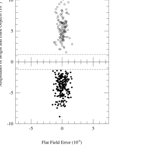
Fig. 10: Maximum amplitudes of spurious peaks caused by hot pixels as a function of the height of hot pixels. Unidentified hot or cold pixels can produce many false peaks in drizzled images. The scatter is due to the pixel geometry distortion in WFPC2 CCD chips (Holtzman et al. 1995). It can be seen that the maximum flux contribution by pixel defects (shown as horizontal dashed lines in Figure 5) is much lower than the typical amplitude of our bright and dark objects.

In Figure 5 we show the flat field errors at the locations of our color-selected bright and dark objects. The typical flat field error is about $0.6\times 10^{-6}$ in flux while the amplitude of our peaks is typically $5\times 10^{-6}$. It is clear that the flat field errors can not be responsible for our bright and dark objects.

4.2. Hot and Cold Pixels

In the HDF data reduction process, most hot and cold pixel defects are identified as those above 5 times the background sky fluctuation ($\sigma$) on images median filtered over $5\times 5$ pixels, and then masked (the growing-pixel mask; see section 4.3 of Williams et al. 1996). Under such a criterion, hot or cold pixels with peak heights below $5\sigma$ can not be found. These unidentified hot or cold pixels can appear in the drizzled images as groups of bright or dark objects in our difference maps. For example, in the $V$ bandpass each unidentified hot pixel will be dithered to form 11 peaks within roughly $2.3^{\prime\prime}$ on the final $2048\times 2048$ frame. If a significant fraction of our sample is produced by these pixel defects, they will cause false angular clustering over that scale.

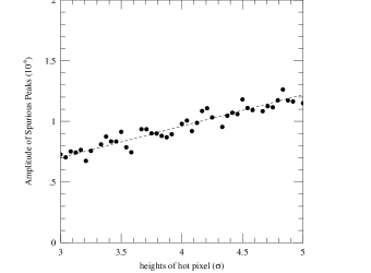
Fig. 12: Maximum amplitudes of spurious peaks caused by hot pixels as a function of the height of hot pixels. Unidentified hot or cold pixels can produce many false peaks in drizzled images. The scatter is due to the pixel geometry distortion in WFPC2 CCD chips (Holtzman et al. 1995). It can be seen that the maximum flux contribution by pixel defects (shown as horizontal dashed lines in Figure 5) is much lower than the typical amplitude of our bright and dark objects.

To estimate the amplitude of hot or cold pixels in our final difference images we have put artificial hot pixels with heights less than $5\sigma$ on a $800\times 800$ array and make the corresponding high resolution map by projecting the dithered images on a $2048\times 2048$ array. This map is smoothed over $0.8^{\prime\prime}$ and $4^{\prime\prime}$ and subtracted from each other to make the difference map. We then find the maximum peak out of the spurious peaks caused by the hot pixels. Figure 6 shows the relation between the height of input artificial hot pixel and the maximum amplitude of resulting peaks on the difference map. It shows that the maximum contribution of 5 (2.5) $\sigma$ hot or cold pixels to the flux is only 1.2 (0.6) $\times 10^{-6}$ in the difference map. The horizontal dashed lines in Figure 5 indicate this level. It is noted that all our bright and dark objects have amplitudes higher than this maximal effect of unmasked hot or cold pixels.

The flat field error and the hot or cold pixels cannot be responsible particularly for the subset of our dark objects mentioned above since they have negative fluxes on the difference maps in B and V, but have positive fluxes in I. Similarly, the color-selected subset of the bright objects are unlikely to be affected by these artifacts.

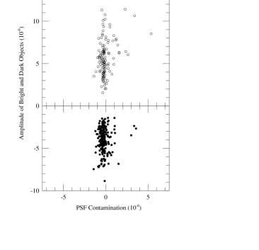
Fig. 14: Contamination by long-range wings of the point spread function at the locations of our color-selected bright and dark objects. Amplitudes of all of our objects are significantly higher than the flux leakages from the masked bright stars and galaxies.

4.3. Contamination by Bright Stars and Galaxies

We have masked objects brighter than roughly $V=29$ on the HDF images to search for fainter objects. However, the PSF of the HDF images is still significant even out to a few arc-seconds. Thus bright stars and galaxies in the HDF images can cast light out of the masked regions and might cause false peaks and correlations in our difference maps.

To see the effects of these wings we use the PSFs calculated by the software Tiny Tim V4.3 recommended by the WFPC2 Instrument Handbook (Biretta et al. 1996). This PSF has a maximum radius of $7.5^{\prime\prime}$. Using this PSF, we have deconvolved the original HDF data to get unblurred images. We then take those pixels which have been masked in our analysis. These pixels contain stars and galaxies brighter than about $V=29$. The map with these bright sources present but with zero flux outside them is prepared, and convolved with the PSF. This blurred image is smoothed over $0.8^{\prime\prime}$ and $4^{\prime\prime}$ and subtracted from each other to make the difference map. From the resulting map we can measure the effects of bright sources on the flux distribution outside our mask regions. We have then measured the flux leakages from bright sources at the locations of our bright and dark objects, and plotted them in Figure 7. It is again clear that our samples and correspondingly their correlations are not artifacts caused by long-range wings of bright stars and galaxies. In particular, large contaminations ($\sim 3\times 10^{-6}$) on the dark objects are all positive, and these objects would have appeared even darker without the contamination.

5. Morphology of Peaks

In the previous section we have shown that the faint diffuse objects we have identified are clustered with an amplitude consistent with that of the present bright galaxies. It supports the idea that these objects are indeed the ancestors of the nearby bright galaxies, undergoing formation at high redshifts. Therefore it is necessary to inspect their morphology to understand the galaxy formation.

Fig. 16: Images of typical bright (top three rows) and dark (bottom three rows) objects in WF3 detected in $V$ (see the text for more description). Each panel is a part of the difference map between the WF3 images smoothed over $0.16^{\prime\prime}$ and $4^{\prime\prime}$, and has a field of view of $3.24^{\prime\prime}\times 3.24^{\prime\prime}$. Objects are at the center, and have sizes of $\sim 0.8^{\prime\prime}$. Bright objects are from the color-selected subset. Dark objects are those with ${}^{-}V$ & ${}^{-}B<31$ but with $I<31$. That is, they are dark in $B$ and $V$ but bright in $I$. Surface brightness or darkness profiles in $V$ are also shown.

In WF3, for example, we have found 40 bright objects with $V<31$ and $B,I<32$, and also satisfying the color-selection criterion. Among these the upper three rows of Figure 8 show high-resoluton $B,V,$ and $I$ images of the 8th (top row, $V=$29.37), 13th (29.45), 18th (29.61) brightest objects. These are from the difference map between the images smoothed over $0.16^{\prime\prime}$ (4 pixels) and $4^{\prime\prime}$ (100 pixels). Each panel has a field of view of $3.24^{\prime\prime}\times 3.24^{\prime\prime}$, and contains one object at the center about four times smaller in length. Figure 8 also shows the surface brightness profile in $V$.

Several common features can be noticed. First, most of these objects do not have bright centers or dominating cores. They are sprinkled with many noise-like glares and show extended backgrounds. Some of them are highly elongated with emission of connections and seem to be undergoing merging. When the local background is further subtracted out within a bright object, each small spot contained in the object typically has the $V$ magnitude of $31\sim 33$. If they are real signals, they are as bright as the bright superassociations which can be found in nearby late type galaxies. Wray & de Vaucouleurs (1980) have found ultrabright blue superassociations in spiral and irregular galaxies having absolute $M_{B}$ magnitudes between $-10$ and $-15$. If these superassociations have the spectra of nearby extragalactic giant star clusters (Rosa & Benvenuti 1994), they would appear as objects with $V=29\sim 34$ (for $h=0.8$) at $z=3.6$, the lower bound of redshift of our color-selected subset. Therefore, the noisy spots embedded in an object have brightness of the superassociations of young blue stars.

Colley et al. (1997) have argued that the objects they have found in the HDF are probably giant star-forming regions. Their argument is based on the comparison with the luminosity, size, surface texture and brightness profile of nearby giant HII regions like 30 Dorados in LMC. Nearby superassociations including 30 Dorados would have $V$ magnitudes fainter than $28.5$ at their assumed redshift $z>2.4$. Since their objects are as bright as $V=25$, their objects are several magnitudes brighter than the superassociations mentioned above. If their objects are giant star-forming regions, the star formation activity in such spots is an order of magnitude stronger than nearby super-starclusters.

The surface profiles of our proto-galaxy candidates are diverse, and do not resemble those of the present bright galaxies. Color fluctuations on the surfaces of the objects are strong. The brightest region in an object often appears at a slightly different location in different bandpasses. Because of our color criterion the color-selected subset of the bright objects are in general fainter in B and I than in V. However, there are often flux excesses in the B and I bandpasses nearby the V-selected peaks. All these characteristics support that these objects are in the process of formation.

The three bottom rows show $0.16^{\prime\prime}$ resolution $B,V$ and $I$ images of three typical objects that are dark in $V$ and $B$, but bright in $I$. In $I$ images they are associated with many emission knots. Their surface ‘darkness profiles’ in $V$ are also diverse like the bright objects. The dark objects are not highly elongated ‘lanes’. This subset of dark objects might be the ‘intergalactic dark clouds’ blocking the background short wavelength light instead of empty dark spaces between galaxies at highest redshifts.

6. Conclusions

We have found very faint ($29<V<31$) extended ($\sim 1^{\prime\prime}$) bright and dark objects in the HDF, and shown that they are real and physically clustered. We have been able to detect these objects by removing all sources brighter than about $V=29$ in the HDF images, smoothing the maps over $0.8^{\prime\prime}$ and $4^{\prime\prime}$, and subtracting between them to remove the local background. With significantly increased signal-to-noise ratios even $0.5\sigma_{d}$ peaks in the difference maps show strong cross-correlations between images in different bandpasses.

Taking into account the amplitude and shape of the angular auto-correlation functions, the morphology, color and surface brightness profiles of these objects, we conclude that they are likely to be the primordial galaxies in the process of formation, and ancestors of the present bright nearby galaxies. The angular CF has a slope of about $-1$, consistent with the slope of the spatial and angular CFs of the present bright galaxies. Its amplitude is also consistent with that of the spatial CF of nearby galaxies extrapolated under various scenarios for the evolution of clustering, and in various cosmologies. More accurately determined CFs of deep objects will be able to discriminate these scenarios and cosmological models. The subset of high redshift objects constrained by colors shows an angular CF significantly stronger than that of the whole sample. These objects are typically sprinkled with many tiny bright knots surrounded by diffuse backgrounds, lacking the predominant core. Their surface brightness profiles are diverse and are far from those of dynamically relaxed objects. They are likely to be in the process of formation.

Recent cosmological simulations of structure formation (Park 1997) have shown that the galactic and sub-galactic scale objects form (undergo complete collapse) at redshifts much before 10 in popular cosmogonies like the standard Cold Dark Matter model (Park 1990; Park et al. 1994). These high redshift objects continue to grow through frequent mergings. Therefore, it is natural to expect to find actively star forming irregular proto-galactic objects in deep images. Our proto-galaxy candidates have many of the characteristics (magnitude, color, morphology, etc.) of these objects seen in the simulations. More deep ground and space infrared images are also predicted to show these objects (cf. Djorgovski et al. 1995).

We have also payed attention to dark patches with negative fluxes below the local background level. Since they tend to persist as the smoothing length is increased, and often have dark pairs at short distances in different bandpasses, they are thought to be real objects. In his deep surveys from 0.32 to 0.9$\mu m$ Tyson (1990) has also noted the presence of reproducible ‘dark lanes’ at scales smaller than $30^{\prime\prime}$. He has argued that they may be intergalactic dust clouds or open tunnels in the galaxy distribution. Our dark objects are found to be weakly self-clustered. The subset of dark objects selected in the $V$ images, which are also dark in $B$ but bright in $I$ (i.e. red), do have a significantly higher auto-correlation function compared to that of the whole dark sample. On the other hand, the objects dark in all filters have a nearly zero CF. The objects dark in $V$ and $I$ but bright in $B$ (i.e. blue) similarly have a vanishing CF. The first subset of dark objects may be intergalactic dark clouds opaque in the far UV (in the rest frame), but emitting or transmitting some light at longer wavelengths. This kind of objects might supply us an important clue to structure formation mechanisms. The second subset of dark objects may be the empty dark spaces between primeval galaxies. If this is the case, we are now looking at the edge of the universe of galaxies.

ACKNOWLEDGEMENTS

This work was supported by the Basic Science Research Institute Program, Ministry of Education 1995 (BSRI-97-5408).

References

- 1 Biretta, J., et al., 1996, WFPC2 Instrument Handbook v4.0, STScI Publication
- 2 Clements, D. L. & Couch, W. J. 1996, MNRAS, 280, L43
- 3 Colley, W. N., Rhoads, J. E., Ostriker, J. P., & Spergel, D. N. 1996, ApJL, 473, L63
- 4 Colley, W. N., Gnedin, O. Y., Ostriker, J. P., & Rhoads, J. E. 1997, ApJ, 488, 579
- 5 Djorgovski, S., et al. 1995, ApJL, 438, L13
- 6 Efstathiou, G., Bernstein, G., Katz, N., Tyson, J. A., & Guhathakurta, P. 1991, ApJL, 380, L47
- 7 Hamilton, A. J. S. 1993, ApJ, 417, 19
- 8 Holtzman, J., et al. 1995, PASP, 107, 156
- 9 Lowenthal, J. D., Koo, D. C., Guzmàn, R., Gallego, J., Phillips, A. C., Faber, S. M., Vogt, N. P., Illingworth, G. D., & Gronwall, C. 1997, ApJ, 481, 673
- 10 Madau, P., Ferguson, H. C., Dickinson, M., Giavalisco, M., Steidel, C. C., & Fruchter, A. 1996, MNRAS, 283, 1388
- 11 Oke, J. B., 1974, ApJS, 27, 21
- 12 Park, C. 1990, MNRAS, 242, 59P
- 13 Park, C. 1997, J. Kor. Astron. Soc., 30, no. 2, in press
- 14 Park, C. & Kim, J. H. 1997, J. Kor. Astron. Soc., 30, no. 1, 83
- 15 Park, C., Vogeley, M. S., Geller, M. J., & Huchra, J. P. 1994, ApJ, 431, 569
- 16 Peebles, P. J. E. 1980, Large-Scale Structure of the Universe, Princeton: Princeton University Press
- 17 Peebles, P. J. E. 1993, Principles of Physical Cosmology, Princeton: Princeton University Press
- 18 Rosa, M. R. & Benvenuti, P. 1994, AAP, 291, 1
- 19 Steidel, C. C., Giavalisco, M., Dickinson, M., & Adelberger, K. L. 1996, AJ, 112, 352
- 20 Tyson, J. A. 1990, in The Galactic and Extragalactic Background Radiation, IAU Symp., No. 139, ed. S. Bowyer & C. Leinert, p245
- 21 Villumsen, J, V., Freudling, W. & da Costa, L. N. 1997, ApJ, 481, 578
- 22 Williams, R. E. et al. 1996, AJ, 95, 107
- 23 Wray, J. D., & de Vaucouleurs, G. 1980, AJ, 85, 1