Detection of Extended Red Emisson in the Diffuse Interstellar Medium

Abstract

Extended Red Emission (ERE) has been detected in many dusty astrophysical objects and this raises the question: Is ERE present only in discrete objects or is it an observational feature of all dust, i.e. present in the diffuse interstellar medium? In order to answer this question, we determined the blue and red intensities of the radiation from the diffuse interstellar medium (ISM) and examined the red intensity for the presence of an excess above that expected for scattered light. The diffuse ISM blue and red intensities were obtained by subtracting the integrated star and galaxy intensities from the blue and red measurements made by the Imaging Photopolarimeter (IPP) aboard the Pioneer 10 and 11 spacecraft. The unique characteristic of the Pioneer measurements is that they were taken outside the zodiacal dust cloud and, therefore, are free from zodiacal light. The color of the diffuse ISM was found to be redder than the Pioneer intensities. If the diffuse ISM intensities were entirely due to scattering from dust (i.e. Diffuse Galactic Light or DGL), the color of the diffuse ISM would be bluer than the Pioneer intensities. Finding a redder color implies the presence of an excess red intensity. Using a model for the DGL, we found the blue diffuse ISM intensity to be entirely attributable to the DGL. The red DGL was calculated using the blue diffuse ISM intensities and the approximately invariant color of the DGL calculated with the DGL model. Subtracting the calculated red DGL from the red diffuse ISM intensities resulted in the detection of an excess red intensity with an average value of $\sim$10 ${\rm S}_{10}({\rm V})_{\rm G2V}$ . This represents the likely detection of ERE in the diffuse ISM since H$\alpha$ emission cannot account for the strength of this excess and the only other known emission process applicable to the diffuse ISM is ERE. Thus, ERE appears to be a general characteristic of dust. The correlation between $N_{HI}$ and ERE intensity is $(1.43\pm 0.31)$$\times 10^{-29}$ ergs s^-1 Å^-1 sr^-1 H atom^-1 from which the ERE photon conversion efficiency was estimated at $10\pm 3$%.

1 Introduction

Extended Red Emission (ERE) is a broad ($\Delta\lambda\sim 800$ Å) emission band with a peak wavelength between 6500 Å and 8000 Å seen in many dusty astrophysical objects (Figure 1). For many years, the Red Rectangle was the only object known to possess such an emission feature (see Schmidt, Cohen, & Margon [1980] for an excellent Red Rectangle spectrum). This all changed with the discovery that many reflection nebulae possessed flux levels in the R and I bands in excess of that expected from dust scattered starlight (Witt, Schild, & Kraiman (1984); Witt & Schild (1985), 1986). The spectroscopic confirmation of the excess flux as ERE (Witt & Schild (1988); Witt & Malin (1989); Witt et al. (1989); Witt & Boroson (1990)) proved that ERE was a feature of many, but not all, reflection nebulae. The identification of the band as emission was strengthened by the imaging polarimetry of NGC 7023 by Watkin, Geldhill, & Scarrott (1991), which showed a reduction in the R and I polarization where R and I excess flux existed. This convincingly proved that the excess flux is due to an emission feature and not changes in the dust scattering properties.

Figure 1: An example of Extended Red Emission is plotted. This spectrum is for the reflection nebula NGC 2327 and has had the underlying scattering continuum subtracted (Witt 1988).

The detection of ERE in other dusty astrophysical objects quickly followed the confirmation of ERE in reflection nebulae. Up to the date of this paper, ERE has been detected in the Red Rectangle (Schmidt et al. (1980)), reflection nebulae (see above), a dark nebula (Mattila (1979); Chlewicki & Laureijs (1987)), Galactic cirrus clouds (Guhathakurta & Tyson (1989); Guhathakurta & Cutri (1994); Szomoru & Guhathakurta (1998)), planetary nebulae (Furton & Witt 1990, 1992), H II regions (Perrin & Sivan (1992); Sivan & Perrin (1993)), a nova (Scott, Evans, & Rawlings (1994)), the halo of the galaxy M82 (Perrin, Darbon, & Sivan (1995)), and the 30 Doradus nebula in the Large Magellanic Cloud (Darbon, Perrin, & Sivan (1998)).

Clues as to the identity of the material that produces ERE are contained in the above observations. The first clue comes from the wide variety of objects that show ERE. The material must be able to survive in radically different environments: from cold, quiescent environments (dark nebulae and Galactic cirrus clouds) to hot, dynamic environments (reflection nebulae, planetary nebulae, and H II regions). Second, the material most likely is carbonaceous since ERE has been detected in carbon rich planetary nebulae but not oxygen rich planetary nebulae (Furton & Witt (1992)). The robustness of carbonaceous dust material is supported by the essentially constant C/H values found for sight lines exhibiting different dust characteristics (Sofia et al. (1997)), implying that carbon is not easily exchanged between the gas and dust phases of the ISM. The third clue comes from the spatial distribution of ERE in reflection nebulae (Witt & Schild (1988); Witt & Malin (1989); Witt et al. (1989); Witt & Boroson (1990); Rogers, Heyer, & Dewdney (1995); Lemaire et al. (1996)) and planetary nebulae (Furton & Witt (1990)). The ERE is strongest in regions where H₂ is being dissociated, leading to the conclusion that warm atomic hydrogen increases the efficiency of ERE luminescence. So, the material that produces ERE must be robust, contain carbon, and produce ERE more efficiently in the presence of atomic hydrogen.

A prime candidate for this material is hydrogenated amorphous carbon (HAC), which was first proposed to explain the ERE in the Red Rectangle (Duley (1985)). With the discovery of ERE in reflection nebulae and other dusty objects, the identification of HAC with ERE has strengthened (Duley & Williams (1988); Witt & Schild (1988); Duley & Williams (1990); Witt & Furton (1994)). The identification of HAC with ERE is strongly supported by the laboratory work of Furton & Witt (1993). They have shown that the low or non-existent photoluminescence of previously annealed HAC or pure amorphous carbon can be greatly enhanced by exposure to atomic hydrogen and/or ultraviolet radiation. This corresponds to the strengthening of ERE in H₂ dissociation regions discussed above. Other ERE producing materials have been proposed, such as filmy quenched carbonaceous composite (Sakata et al. (1992)) and C₆₀ (Webster (1993)). For a discussion of the similarities and differences between these materials see Papoular et al. (1996).

As ERE has been detected in a large range of dusty objects, the question arises: Is ERE present in the diffuse interstellar medium (ISM)? If the answer is yes, this would make ERE a general characteristic of dust. A positive answer has been claimed by Duley & Whittet (1990), who identified the very broad structure (VBS) seen in extinction curves (e.g. van Breda & Whittet (1981)) as due to ERE. Jenniskens (1994) has pointed out that ERE cannot be the cause of the VBS for two reasons. First, spectra showing VBS have had the nearby sky subtracted, effectively removing any emission from the diffuse ISM. Second, the VBS strength does not depend on the size of the aperture used. Hence, ERE has not been detected in the diffuse ISM. As a result, dust models for the diffuse ISM have not used the ability to produce ERE as a constraint on possible dust grain materials (e.g. Kim & Martin (1996); Mathis (1996); Zubko, Krełowski, Wegner (1996); Dwek et al. (1997); Li & Greenberg (1997)).

This investigation is aimed at determining whether ERE is present in the diffuse ISM. Detecting ERE in the diffuse ISM is much more difficult than doing the same in a discrete object. For a discrete object, ERE detection is done by subtracting a nearby sky spectrum from a spectrum of the object (e.g. Witt & Boroson (1990)). Subtracting a nearby sky spectrum removes contributions to the object spectrum from the Earth’s atmosphere (airglow), zodiacal light (dust scattered sunlight), and Galactic background light (diffuse ISM, faint stars, and galaxies). This results in a spectrum with contributions only from the object being studied, and any ERE is directly attributable to that object. As the light from the diffuse ISM is part of the sky spectrum, this method will not work for it. A different method is required.

Two of the strongest (and most difficult to model) sources in a sky spectrum are airglow and zodiacal light (Toller (1981)). Both of these sources can be avoided by simply taking observations outside the atmosphere (for airglow) and the zodiacal dust cloud (for zodiacal light). Such measurements have already been carried out by the Imaging Photopolarimeters (IPP) carried aboard both Pioneer 10 and 11 (Pellicori et al. (1973); Weinberg et al. (1974)). The IPP measured the intensity of almost the entire sky in the blue (437 nm) and the red (644 nm). By using only measurements taken when the Pioneer spacecraft were beyond 3.27 AU, contributions from the zodiacal light are avoided (Hanner et al. (1974)). Therefore, the only known sources contributing to the IPP measurements are stars, galaxies, and the diffuse ISM. Using photometric star and galaxy catalogs, the contribution to the IPP measurements from stars and galaxies can be removed. The resulting blue and red intensities are due only to the diffuse ISM.

While the IPP measurements have given all-sky maps at two wavelengths and not a spectrum, this is sufficient to detect ERE in the diffuse ISM. The presence of ERE in reflection nebulae was first detected by observing that these objects had red fluxes in excess of that expected from dust scattered starlight (Witt, Schild, & Kraiman (1984)). The diffuse ISM is a gigantic reflection nebula with the Galaxy’s starlight scattered by the Galaxy’s dust. Therefore, we can use the same criterion, excess red flux, to detect ERE in the diffuse ISM. The scattered light in the diffuse ISM is termed Diffuse Galactic Light (DGL). The DGL will have a bluer color than the integrated starlight because scattering by dust is more efficient at shorter wavelengths. So, if the diffuse ISM color (red/blue ratio) is as red as or redder than the integrated starlight and other sources of excess red light can be positively excluded, ERE is present.

Section 2 describes the Pioneer IPP measurements and the construction of the blue and red all-sky maps. The compilation of a star and galaxy photometric catalog, complete to approximately 20th magnitude, is detailed in section 3. The detection of ERE in the diffuse ISM is contained in section 4. Section 5 presents the properties of the ERE in the diffuse ISM. Finally, section 6 discusses the implications of our results and summarizes our conclusions.

2 Pioneer Data

One of the instruments onboard the Pioneer 10 and 11 spacecraft was the Imaging Photopolarimeter (IPP). The primary objectives of the IPP were to produce blue and red maps of the brightness and polarization of the zodiacal dust cloud from 1 to 5 AU, the background light outside the zodiacal dust cloud, and Jupiter (Pellicori et al. (1973)). Of these, we were concerned with only the all-sky blue and red surface brightness maps taken outside the zodiacal dust cloud.

The IPP was a Maksutov-type f/3.4 telescope with an aperture of 2.54 cm and a detector consisting of a Wollaston prism, multilayer filters, and two dual-channel Bendix channeltrons (Pellicori et al. (1973); Weinberg et al. (1974)). Simultaneous measurements were made of the orthogonal components of the electric field in both the blue and red. The spectral bandpass (half-power) was 3950–4850 Å for the blue channel and 5900–6900 Å for the red channel (Pellicori et al. (1973)). See subsection 3.1 for more information on the photometric characteristics of the IPP. The IPP instantaneous field of view (FOV) was $2\fdg 29\times 2\fdg 29$ for the background light measurements. The IPP was mounted on a movable arm and 64 measurements were taken during a single rotation of the Pioneer spacecraft. The angle between the arm and the Pioneer spacecraft spin axis (look angle = L) was changed in increments of $1\fdg 83$ to build up a map of the sky. The look angle ranged between $29\arcdeg$ and $170\arcdeg$ (Pellicori et al. (1973)). The effective FOV of the measurements was $2\fdg 29\times(2\fdg 29+5\fdg 625\sin L)$, with a maximum of $2\fdg 29\times 7\fdg 92$ when the look angle was $90\arcdeg$ and a minimum of $2\fdg 29\times 3\fdg 27$ when the look angle was $170\arcdeg$. At each look angle, a 20 data roll (rotation) measurement cycle was performed with 8 rolls for the background light, 1 for a radioisotope-activated phosphor source (¹⁴C), 1 for offset and dark current levels, and 10 for data readout (Pellicori et al. (1973); Weinberg et al. (1974); Toller (1981)).

The raw IPP background sky measurements were processed to produce the Pioneer 10/11 Background Sky data set available from the National Space Science Data Center (NSSDC). The details of the processing can be found elsewhere (Weinberg et al. (1974); Toller (1981); Weinberg & Schuerman (1981); Schuerman, Giovane, & Weinberg (1997)). A brief description of the processing follows. First, the data were calibrated using the inflight measurements of the radioisotope-activated phosphor source. Second, the FOV center was computed from the spacecraft spin axis direction, the look angle, and the clock angle. Third, the contribution from bright stars was subtracted using the stars in the Bright Star Catalogue (Hoffleit & Warren (1991)) and stars with $m_{V}<8$ (Toller, Tanabe, & Weinberg (1987)) in the Photoelectric Catalog (Blanco et al. (1968); Ochsenbein (1974)). Fourth, 37 resolved stars were used to determine the time decay of the instrument sensitivity and corrections to the telescope pointing. The final error in the positions of the FOVs was on the order of $0\fdg 15$–$0\fdg 40$. The Pioneer 10 red data have abnormally high noise, but as we are also using Pioneer 11 data, this did not adversely affect our results. The final Pioneer data are expressed in ${\rm S}_{10}({\rm V})_{\rm G2V}$ units, the equivalent number of 10th magnitude (V band) solar-type stars per square degree. See subsection 3.1 for details of this unit.

During the cruise portion of the Pioneer 10 and 11 missions, the IPP mapped the background light a number of times. In order to determine the spatial extent of the zodiacal dust cloud, Hanner et al. (1974) examined the brightness of two different regions of the sky as seen by the IPP when Pioneer 10 was between 2.41 and 4.82 AU. They found that the brightness of these two regions stopped changing after Pioneer 10 passed 3.27 AU, making this distance the outermost detectable edge of the zodiacal dust cloud. Therefore, all the measurements taken beyond 3.27 AU are free from detectable zodiacal light and useful for this investigation.

On 5 days while Pioneer 10 was between 3.26 and 5.15 AU and on 6 days while Pioneer 11 was between 4.06 and 4.66 AU, the IPP mapped the background light in the sky. The resolution of a map made on a single day is determined by the FOV of the IPP and its overlap with neighboring FOVs. Figure 2a gives an example of the pattern of FOVs using the Pioneer 10 measurements from day 68 of 1974. One of the FOVs has been shaded to show the overlap of a FOV with neighboring FOVs. The resolution of this map is variable, with each parallelogram being a resolution element. In order to actually achieve this theoretical resolution, an algorithm must be used to extract the information in the overlapping regions. In fact, the resolution of the IPP measurements can be increased significantly by using measurements made on different days. Figure 2b gives the pattern of FOVs for the 11 days used in creating the final high-resolution maps (see below). The FOVs from different days do not overlap exactly as the Pioneer 10 and 11 missions were launched on different trajectories and the spin axis of each spacecraft changed direction slowly as a function of distance from the Sun.

Figure 2: The pattern of the FOVs are plotted in these two figures. The pattern of FOVs from Pioneer 10 on day 68 of 1974 is shown in (a) with points in the center of the FOVs. One FOV is shaded to show the regions which overlap neighboring FOVs. The pattern of FOVs from the 11 days used in constructing the final maps is shown in (b). Due to the different trajectories of Pioneer 10 and 11 and the variable spacecraft spin axis orientation, the FOVs from different days do not overlap exactly.

2.1 Map Generation Algorithm

The algorithm used to create the final maps is similar to that by Aumann, Fowler, & Melnyk (1990). Their algorithm is called the Maximum Correlation Method (MCM) and it was able to improve the resolution of IRAS maps by a factor of $\sim 6.5$, from $\sim 4\arcmin$ to $\sim 36\arcsec$. Our algorithm was similar to MCM and worked in the following manner. An initial guess at the final image (zeroth iteration) was taken as a positive flat image with $0\fdg 25\times 0\fdg 25$ pixels. The next iteration was calculated from

$$p_{ij}^{k+1}=\left(\frac{1}{N}\sum_{m=1}^{N}C_{m}\right)p_{ij}^{k}$$ (1)

where $p_{ij}^{k}$ is the surface brightness of the $k$th iteration image at pixel coordinates ($i$,$j$), $C_{m}$ is the correction factor for the $m$th IPP measurement (the surface brightness in particular FOV) which includes $p_{ij}$, and the sum was done over the $N$ IPP measurements which include $p_{ij}$. The value of $C_{m}$ was calculated from

$$C_{m}=I_{m}\left(\frac{1}{Q}\sum^{Q}p_{ij}^{k}\right)^{-1}$$ (2)

where $I_{m}$ is the $m$th IPP measurement and the sum was done over the $Q$ pixels which are included in the $m$th IPP FOV. The error, $\sigma_{ij}^{k}$, in $p_{ij}^{k}$ was calculated from

$$\sigma_{ij}^{k}=\frac{1}{N}\sqrt{\sum_{m=1}^{N}\left(I_{m}-\left[\frac{1}{Q}\sum^{Q}p_{ij}^{k}\right]_{m}\right)^{2}}.$$ (3)

With each iteration, the image gives an improved match to the IPP measurements. The outcome of this algorithm is to produce an image which describes all 11 days of the Pioneer measurements.

Table 1: IPP Usable Days

Spacecraft	year	day	R
	[years]	[days]	[AU]
Pioneer 10	1972	354	3.26
Pioneer 10	1973	149	4.22
Pioneer 10	1973	237	4.64
Pioneer 10	1973	279	4.81
Pioneer 11	1974	57	3.50
Pioneer 10	1974	68	5.15
Pioneer 11	1974	106	3.81
Pioneer 11	1974	148	4.06
Pioneer 11	1974	178	4.22
Pioneer 11	1974	236	4.51
Pioneer 11	1974	267	4.66

The 11 days of IPP background light measurements that were used in constructing the final high-resolution maps are tabulated in Table 1. While the 11 days overall possessed usable data, a large number of individual measurements were seen to be of poor quality. There are a number of sources for the poor quality data: incorrect subtraction of bright stars, scattered sunlight, and corrupt data rolls (Toller (1981)). The poor quality data were removed from consideration using four criteria. First, data contaminated with scattered sunlight (data taken within $70\arcdeg$ of the sun for Pioneer 10 and within $45\arcdeg$ for Pioneer 11) were removed. Second, all data with negative values were removed as these were the result of interuptions in the datastream of between the spacecraft and ground station. Third, the data were divided into $5\arcdeg\times 5\arcdeg$ boxes and data inside each box deviating over 3 standard deviations from the average in either their blue measurements, red measurements, or red/blue ratio were removed. Fourth, a small number of points were removed by visual inspection. Approximately 25% of the IPP measurements were of poor quality.

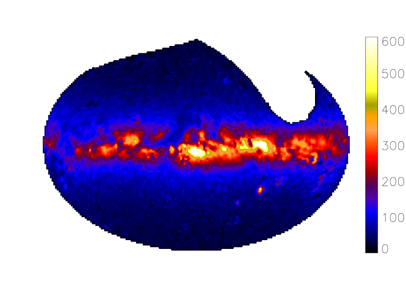
Figure 3: The Aitoff projection (galactic longitude of zero in the center) of the Pioneer blue image of the sky is displayed. The resolution of the displayed map is $0\fdg 5$ by $0\fdg 5$. The large hole corresponds to the Sun’s location as seen from Pioneer 10/11. The intensity units are ${\rm S}_{10}({\rm V})_{\rm G2V}$ .

The resulting good data were used as the input for the algorithm described above to produce the final high-resolution maps. The algorithm was iterated 10 times, until little change was detected. The best iteration map to use depended on the region being investigated. For low galactic latitude regions where the amplitude of real structure in the maps is much larger than the noise amplitude, the 10th iteration gave the best map. For high galactic latitude regions where the real structure amplitude is smaller than the noise amplitude, the 1st iteration gave the best map.

The 10th iteration map for the blue is displayed in Figure 3. The 10th iteration red map is similar to the blue map. Typical uncertainties were 2% for the blue and 3% for the red. Figure 3 can be compared directly with the blue background as seen by the Hipparcos star mapper. A map of this background is presented in Figure 6 of Wicenec & van Leeuwen (1995). The comparison is good both in overall strength and morphology. From this comparison, the uniqueness of the Pioneer maps was quite apparent as the Pioneer blue map lacks the substantial zodiacal light seen in the Hipparcos star mapper blue map.

As we were only concerned with high latitude regions, we will use the 1st iteration map for the rest of this paper and save the higher iterations for later work. The 1st iteration blue and red maps are just smoother versions of the 10th iteration maps.

3 Photometric Star and Galaxy Counts

In order for this investigation to succeed, the contribution to the Pioneer blue and red measurements from stars and galaxies fainter than $m_{V}=6.5$ was needed. We have tackled this problem by constructing a Master Catalog from three separate catalogs, each complete in a subset of the range between 6.5 and $\sim$20th magnitude. Ironically, the stars and galaxies with magnitudes between 12 and $\sim$20 (Palomar O & E) have the best photometric data available due to the existence of the Automated Plate Scanner Catalog of the Palomar Sky Survey I (APS Catalog, Pennington et al. (1993)). In the magnitude range between 9 and 15 ($\sim$V band in the north and $\sim$B in the south), the Guide Star Catalog (GSC, Lasker et al. (1990); Russell et al. (1990); Jenkner et al. (1990)) provides data in only one band. For the magnitude range between 6.5 and 9.5, there exists no good complete photometric catalog. We have used a combination of catalogs (see §3.2) to construct a Not So Bright Star Catalog (NSBS Catalog) to give the best currently available positions and magnitudes for stars with magnitudes between 6.5 and 9.5.

3.1 Transformations Between Photometric Systems

Figure 4: The response curves are plotted for the Pioneer blue and red channels (PB & PR, Toller 1981), the Johnson B and R (Lamla 1982) and the Palomar blue and red (O & E, Minkowsi & Abell 1963).

Underlying the construction of the Master Catalog was the transformation between the Palomar blue & red (O & E) magnitudes and Johnson B & R magnitudes to Pioneer blue & red (PB & PR) magnitudes. The normalized response curves, $R(\lambda)$, for the blue and red bands of all three photometric systems are shown in Figure 4 (Minkowsi & Abell (1963); Lamla (1982); Toller (1981)). The Palomar blue (O) response function was computed for an airmass of 1.5 (Hayes & Latham (1975)) in order to reproduce the transformation between the Palomar and Johnson systems used in calibrating the APS Catalog (Humphreys et al. (1991)). For all 6 above bands as well as the Johnson V band, the band’s equivalent wavelength ($\lambda_{\rm eq}$), equivalent bandpass ($\Delta\lambda_{\rm eq}$), zero magnitude flux (F_λ), and the intensity corresponding to ${\rm S}_{10}({\rm V})_{\rm G2V}$ and ${\rm S}_{10}({\rm V})_{\rm A0V}$ units were computed and are tabulated in Table 2. The values of $\lambda_{\rm eq}$ and $\Delta\lambda_{\rm eq}$ are obtained by

$$\lambda_{\rm eq}=\frac{\int\lambda R(\lambda)\,d\lambda}{\int R(\lambda)\,d\lambda}$$ (4)

and

$$\Delta\lambda_{\rm eq}=\frac{\int R(\lambda)\,d\lambda}{R_{\rm max}},$$ (5)

respectively. The flux corresponding to a magnitude of zero, F_λ, in each band was calculated by summing the product of the band’s response curve and a calibrated spectrum of $\alpha$ Lyrae (Tüg, White, & Lockwood (1977)). The calibrated spectrum of $\alpha$ Lyrae was multiplied by 1.028 before use to account for the fact that $\alpha$ Lyrae’s V magnitude is 0.03 (Hoffleit & Warren (1991)). The intensity corresponding to one ${\rm S}_{10}({\rm V})_{\rm G2V}$ unit and one ${\rm S}_{10}({\rm V})_{\rm A0V}$ unit was computed by summing the product of each band’s response curve with the spectrum, set to 10th magnitude in the V band, of the sun (Lockwood, Tüg, & White (1992)) and $\alpha$ Lyrae (Tüg, White, & Lockwood (1977)), respectively. One ${\rm S}_{10}({\rm V})_{\rm X}$ unit is defined as intensity equivalent to one 10th V magnitude star of spectral type X per square degree where X is either G2V or A0V. The intensity in mag/$\sq\arcsec$ corresponding to ${\rm S}_{10}({\rm V})_{\rm G2V}$ units in the B bands, V band, and R bands is 28.5, 27.8, and 27.5 mag/$\sq\arcsec$, respectively.

Table 2: Photometric Band Details

System	Band	$\lambda_{\rm eq}$	$\Delta\lambda_{\rm eq}$	Fλ	${\rm S}_{10}({\rm V})_{\rm G2V}$	${\rm S}_{10}({\rm V})_{\rm A0V}$
		[Å]	[Å]	[ergs cm-2 s-1 Å-1]	[ergs cm-2 s-1 Å-1 sr-1]
Johnson	B	4467	1014	6.632$\times 10^{-9}$	1.198$\times 10^{-9}$	2.174$\times 10^{-9}$
Palomar	O	4249	1168	6.343$\times 10^{-9}$	1.087$\times 10^{-9}$	2.080$\times 10^{-9}$
Pioneer	PB	4370	826	6.997$\times 10^{-9}$	1.192$\times 10^{-9}$	2.294$\times 10^{-9}$
Johnson	V	5553	881	3.639$\times 10^{-9}$	1.193$\times 10^{-9}$	1.193$\times 10^{-9}$
Johnson	R	6926	2057	1.950$\times 10^{-9}$	8.813$\times 10^{-10}$	6.394$\times 10^{-10}$
Palomar	E	6412	386	2.289$\times 10^{-9}$	9.828$\times 10^{-10}$	7.505$\times 10^{-10}$
Pioneer	PR	6441	968	2.305$\times 10^{-9}$	9.919$\times 10^{-10}$	7.558$\times 10^{-10}$

The transformations from the Palomar and Johnson systems to the Pioneer system were accomplished by means of the above band response functions (Figure 4) and zero magnitude fluxes (Table 2) along with an observational grid of stellar spectra spanning the Hertzsprung-Russell diagram (Silva & Cornell (1992)). This grid consists of spectra covering 3510-8930 Å with a resolution of 11 Å and includes 72 spectral types spanning spectral classes O–M and luminosity classes I–V. Most of the spectra are for solar metallicity stars, but some are for metal-rich and metal-poor stars. The spectra were dereddened and stars of similar spectral types were averaged to produce the final 72 spectral type spectra (Silva & Cornell (1992)).

Figure 5: The transformation from the Johnson system to the Palomar system is plotted. The ($O\!-\!B$) correction is displayed in (a) and the ($E\!-\!R$) correction is displayed in (b). Note that the ($O\!-\!B$) and ($E\!-\!R$) corrections derived in this paper agree quite well with those from Humphreys et al. (1991).

In order to check the accuracy of our transformations, the transformation from the Johnson system to the Palomar system was computed and compared to the same transformation as determined by Humphreys et al. (1991). Figure 5a displays the ($O\!-\!B$) correction as a function of (B V) which transforms the Johnson B magnitude to the corresponding Palomar O magnitude. Figure 5b displays the ($E\!-\!R$) correction as a function of (V R) which transforms the Johnson R magnitude to the corresponding Palomar E magnitude. The agreement between the ($O\!-\!B$) and ($E\!-\!R$) corrections derived in this paper and those of Humphreys et al. (1991), validates this method for deriving transformations between photometric systems.

Figure 6: The transformation from the Palomar system to the Pioneer system is plotted. The ($PB\!-\!O$) correction is displayed in (a) and the ($PR\!-\!E$) correction is displayed in (b). The maximum corrections for both ($PB\!-\!O$) and ($PR\!-\!E$) are small.

Figure 7: The transformation from the Johnson system to the Pioneer system is plotted. The ($PB\!-\!B$) correction is displayed in (a) and the ($PR\!-\!R$) correction is displayed in (b). While the maximum correction for ($PB\!-\!B$) is small, the maximum correction for ($PR\!-\!R$) is large due to the significantly different values of $\lambda_{\rm eq}$ for the PR and R response curves.

The transformation from the Palomar to the Pioneer system is displayed in Figure 6 and the transformation from the Johnson to the Pioneer system is shown in Figure 7. We have fitted the resulting curves with polynomial functions in order to have an analytic form for the transformations. The number of terms in the fitted polynomial was determined by adding terms until the resulting fitted polynomial followed the general trend of the points. The maximum corrections for ($PB\!-\!O$), ($PR\!-\!E$), ($PB\!-\!B$), and ($PR\!-\!R$) are $\sim$0.25, $\sim$0.10, $\sim$0.20, and $\sim$1.0, respectively. The large maximum correction for ($PR\!-\!R$) is due to the large difference in the $\lambda_{\rm eq}$ value between the Pioneer (6441 Å) and Johnson (6926 Å) systems.

3.2 Master Catalog Construction

Three star and galaxy catalogs were used in constructing the Master Catalog. The three catalogs were the Not So Bright Star Catalog (NSBS Catalog, see below), the GSC, and the APS Catalog. As the Master Catalog includes a large number of objects, we chose to construct it in small pieces. The GSC is split into 9537 regions (Jenkner et al. (1990)) and we used the same regions for our Master Catalog.

For stars and galaxies with PB magnitudes between 13 and $\sim$20th magnitude, the APS Catalog of the Palomar Sky Survey I (POSS I) was used. This ambitious survey is using POSS I plates to produce a catalog of stars and galaxies with positions and Palomar O and E magnitudes between 12th magnitude and the plate limit ($\sim$20th magnitude). Due to difficulties in automated photometry in crowded fields, the APS Catalog is limited to $|b|>20\arcdeg$ (Pennington et al. (1993)). The APS Catalog is also limited by the lack of any POSS I plates below a declination $-33\arcdeg$ (Minkowsi & Abell (1963)). The spatial extent of the APS Catalog defines the regions where we can accurately remove the integrated contributions of stars and galaxies to the Pioneer data. The positional accuracy is $0\farcs 5$ (Pennington et al. (1993)). The O and E magnitudes were calibrated using UBV photoelectric photometry as detailed in Humphreys (1991). The resulting random error in magnitudes was 0.2 for stars and 0.3-0.5 for galaxies (Pennington et al. (1993)). The star/galaxy classification was done using a neural network (Odewahn et al. (1992), 1993). Regions surrounding bright stars are not included in the APS Catalog due to scattered light from the bright stars. We identified these holes by hand and stars and galaxies from a nearby region of equal size were copied into the hole.

The Guide Star Catalog (GSC) was used to provide data for stars and galaxies with PB magnitudes between 9.5 and 13. For each object, the GSC contains a position and a V ($\left<\lambda\right>\approx 5600$ Å) or a J ($\left<\lambda\right>=4500$ Å) magnitude (Lasker et al. (1990)). The position error is $0\farcs 2-0\farcs 8$ and the magnitude error is $\sim$0.30 mag (Russell et al. (1990)). As the GSC gives only one magnitude, deriving accurate PB and PR magnitudes for each object was not possible. Since the GSC is complete to 15th magnitude, a large number of the GSC objects also appear in the APS catalog. This fact allowed us to statistically transform the GSC object magnitudes to the Pioneer system. The average ($PB\!-\!V$) or ($PB\!-\!J$) and ($PB\!-\!PR$) color for stars in common to both the GSC and APS Catalog was computed and used to transform the magnitudes of the GSC objects to the Pioneer system.

The catalog of stars between 6.5 V magnitude and 9.5 PB magnitude was constructed by combining three different existing catalogs: the Catalogue of Stellar Identifications (CSI, Ochsenbein (1983)), the Michigan Catalogue of Two-Dimensional Spectral Types for HD Stars (Houk Catalog, Houk & Cowley (1975); Houk (1978); Houk (1982); Houk & Smith-Moore (1988)), and the UBV Photoelectric Photometry Catalogue (UBV Catalog, Mermilliod (1987); Mermilliod (1994)). This produced the Not So Bright Star Catalog (NSBS Catalog) with each star possessing the most accurate position, spectral type, PB magnitude, and PR magnitude possible. The CSI was used as the base for the NSBS Catalog. It is complete to $m_{\rm V}\approx 9.5$ (Ochsenbein, Bischoff, & Egret (1981)) and is the combination of many other catalogs, notably the Henry Draper Catalog (HD Catalog, Cannon & Pickering 1918- (1924); Cannon 1925- (1936); Cannon & Walton Mayall (1949)) and the Smithsonian Astrophysical Observatory Catalogue (SAO Catalog, SAO Staff (1966)). Stars already subtracted from the Pioneer data were excluded from the NSBS Catalog by excluding all stars in the Bright Star Catalogue (Hoffleit & Warren (1991)) and stars with $m_{V}<8$ (Toller, Tanabe, & Weinberg (1987)) in the Photoelectric Catalog (Blanco et al. (1968); Ochsenbein (1974)).

Figure 8: The transformation between the Johnson (B V) to (V R) color is plotted above. The open circles were calculated by summing the product of the appropriate response curves and the grid of stellar spectra (Silva & Cornell 1992).

Information for each star in the NSBS Catalog was gathered in the following manner. The star’s position was taken from the CSI. The star’s spectral type was taken (in order of preference) from the Houk Catalog or the CSI. The star’s PB and PR photometry was determined from the star’s Johnson B and R magnitudes which were calculated using one of the following algorithms. If the star’s V magnitude and (B V) color were available from the UBV Catalog, the R magnitude was computed by using the fit given in Figure 8 to calculate the star’s (V R) color. If only the star’s V magnitude was available, then the star’s (B V) color was computed from

$$(\bv)=(\bv)_{o}+E(\bv)$$ (6)

where (B V)_o is the star’s unreddened color and $E(\bv)$ is the reddening due to dust. A similar equation was used to compute the star’s (V R) color.

Figure 9: The relationship between a luminosity class V star’s temperature class and (a) (B V) and (b) (V R). The spectral type code (spcode) is a numerical representation of the star’s temperature class with O = 0, B = 10, A = 20, etc. and subclasses worth their values. For example, a A4 temperature class has a spcode = 24.

The unreddened $(\bv)_{o}$ and $(\vr)_{o}$ were determined using fits between spectral type and unreddened color computed using the Johnson response curves and the grid of stellar spectra (Silva & Cornell (1992)). Figure 9 displays the fits to the (B V)_o and (V R)_o colors for luminosity class V. Fits for luminosity classes III and I were similar. Ideally, all the stars in the NSBS Catalog would have two-dimensional MK spectral types resulting in accurate unreddened colors. This is true for stars in the HD Catalog (complete to $m_{\rm pg}\approx 9$ [Roman & Warren (1985)]) with declinations less than $-12\arcdeg$ (Houk Catalog) and a few other stars in the CSI with spectral types from other sources (Ochsenbein (1983)). For the stars with only one-dimensional temperature classes, the unreddened (B V)_o and (V R)_o colors were calculated by taking a weighted average of the (B V)_o and (V R)_o colors corresponding to luminosity classes V, III, and I. The weights were the probability of finding a V, III, or I luminosity class star of the star’s temperature class with the star’s V magnitude and absolute value of galactic latitude. These probabilities were determined from the Houk Catalog.

For each star, $E(\bv)$ and $E(\vr)$ values were calculated from

$$E(\bv)=\left[\frac{E(\bv)}{A_{V}}\right]A_{V}=0.33A_{V}$$ (7)

and

$$E(\vr)=\left[\frac{E(\vr)}{A_{V}}\right]A_{V}=0.17A_{V},$$ (8)

respectively (Whittet (1992)). The values for $E(\bv)/A_{V}$ and $E(\vr)/A_{V}$ correspond to an average Milky Way extinction curve, $R_{V}=3.05$ (Whittet (1992)). $A_{V}$ is calculated using

$$A_{V}=\alpha d$$ (9)

where $\alpha=0.6~{}\mbox{mag kpc}^{-1}$ and $d$ is the star’s distance. In order to determine the value of $\alpha$ given above, we extracted all 19,746 stars in the NSBS Catalog with two-dimensional spectral types and an observed (B V). Using these stars’ two-dimensional spectral types, we calculated their (B V) colors from the algorithm described above with a range of $\alpha$ values. For an $\alpha=0.6~{}\mbox{mag kpc}^{-1}$, the calculated and observed (B V) colors were equal with no galactic latitude dependence of $\alpha$ necessary. The distance was computed by solving

$$m_{V}-M_{V}=5\log\left(\frac{d}{10~{}\mbox{pc}}\right)+\alpha d$$ (10)

where $m_{V}$ is the observed V magnitude and $M_{V}$ is the absolute magnitude appropriate for the star’s spectral type (Schmidt-Kaler (1982)). Again, for stars without two-dimensional spectral types, the computed $E(\bv)$ and $E(\vr)$ values were a weighted average of color excesses for V, III, and I luminosity classes. Finally, the star’s B and R magnitudes were transformed to Pioneer PB and PR magnitudes using the transformations given in §3.1.

We were only interested in the integrated star/galaxy intensity and chose to do the integration over $5\arcdeg\times 5\arcdeg$ sized regions (see section 4). Since the integration was done over regions larger than an individual Master Catalog region which contains $\sim$20,000 objects, the error in the integrated intensity was dominated by systematic errors. The random error in the integrated intensity due to random errors in the fluxes of individual objects was very small due to the large number of objects contributing to the integrated intensity.

The only systematic error found was associated with the lack of two-dimensional spectral types for many of the stars in the NSBS Catalog. By using the population statistics from the Houk Catalog (see above), the magnitude of this error was greatly reduced. Using the Master Catalog regions with spectral types from the Houk Catalog, we determined the remaining systematic error. The integrated flux for the stars in these Master Catalog regions with PB magnitudes between 5.5 and 9.5 was determined two ways, using the stars’ two-dimensional spectral types and using only the stars’ one-dimensional spectral types. On average, the integrated PB star flux using the one-dimensional spectral types was $2.5\pm 1.5\%$ too high and the integrated PR flux was $3.3\pm 2.5\%$ too low. Since there was a systematic zero point error, the PB and PR magnitudes for stars without two-dimensional spectral types in the NSBS Catalog were corrected by adding 0.0273 and -0.0349 to their PB and PR magnitudes, respectively. This left a random error of $1.5\%$ and $2.5\%$ in the integrated PB and PR star flux from the NSBS Catalog, respectively.

Figure 10: The combined star/galaxy counts for the NSBS Catalog, the GSC, and the APS Catalog are displayed for two Master Catalog regions. A region at $b=19\fdg 6$ (GSC #2947) is displayed in (a) and a region at $b=74\fdg 6$ (GSC #2526) in (b). The counts were normalized to reflect the counts for one square degree and one magnitude wide bins. The error bars were computed assuming Poisson statistics.

In order to show that the construction of the Master Catalog worked, we display the star/galaxy counts for two Master Catalog regions in Figure 10. Figure 10a shows the counts for a low latitude region and Figure 10b shows the counts for a high latitude region. These two figures show the counts from the NSBS Catalog, the GSC, and the APS Catalog in the regions where these catalogs are stated to be valid. The overlap of the three catalogs is good and within the expected uncertainties. Additional confirmation of the Master Catalog comes from comparison of our star counts with that of the SKY model (Cohen (1994), 1995). The star counts predicted from the SKY model agree within Poisson statistics with our observed Master Catalog counts (Cohen (1997)). See Toller (1981) for an excellent review of previous star count work.

Figure 11: The contribution to the total intensity from each half magnitude bin is plotted for the same two regions as in the previous figure. The region at $b=19\fdg 6$ is displayed in (a) and the region at $b=74\fdg 6$ in (b). The peak contribution comes from about 10th magnitude and the contribution from objects with magnitudes $>$ 20 is negligible.

Figure 11 plots the contribution to the total intensity from each half magnitude bin for the same regions displayed in Figure 10. On average, the maximum contribution comes from $\sim$10th magnitude objects. The scatter in the curve for magnitudes $<10$ is due to the relatively small number of bright stars per Master Catalog region. The contribution from stars and galaxies with magnitudes $>20$ is negligible and not the result of the Master Catalog incompleteness as the curve falls smoothly at magnitudes well below 20.

4 Detection of ERE in the Diffuse ISM

The blue and red intensities of the diffuse ISM were determined by subtracting the integrated star/galaxy light (ISGL) from the Pioneer maps. As the ISGL was computed from the Master Catalog, the spatial extent of the diffuse ISM intensities was limited to regions of the sky covered by the APS Catalog. Currently, the APS Catalog includes approximately 400 plates from the POSS I in a fairly random pattern across the sky. Due to the low resolution of the Pioneer maps and the size of an individual POSS I plate ($6\fdg 6$, Minkowsi & Abell (1963)), regions with many adjoining plates were needed. Currently, only two regions have enough contiguous plates to accurately derive the diffuse ISM intensities. Region 1 is located between $(l,b)=(355\arcdeg,30\arcdeg)$ and $(10\arcdeg,60\arcdeg)$ and region 2 is located between $(l,b)=(90\arcdeg,-55\arcdeg)$ and $(120\arcdeg,-20\arcdeg)$. These two regions have areas of $315~{}\sq\arcdeg$ and $820~{}\sq\arcdeg$ and contain over 110,000 and 746,000 objects, respectively.

In these two regions, maps of the blue and red intensities for the ISGL were computed using the Master Catalog. The fluxes of the stars and galaxies in the Master Catalog were mapped onto a grid in galactic longitude and latitude with $0\fdg 25\times 0\fdg 25$ sized pixels. The fluxes were converted to ${\rm S}_{10}({\rm V})_{\rm G2V}$ units using the conversions given in Table 2 and solid angles (in steradians) computed from

$$\Omega=\left(l_{2}-l_{1}\right)\left(\sin b_{2}-\sin b_{1}\right)$$ (11)

where $l$ is galactic longitude (in radians), $b$ is galactic latitude (in radians), and the subscripts 1 and 2 refer to the minimum and maximum values, respectively. Equation 11 is valid for rectangles in galactic longitude and latitude. The resulting ISGL map was smoothed to a resolution of $2\arcdeg$ to match the Pioneer maps.

In computing the ISGL intensities, we did not include a weighting in accordance with the dwell time of each star within the FOV of individual IPP measurements for the stars fainter than m = 6.5. The corrections for the brighter stars (m $<$ 6.5) which were subtracted in the original reduction of the IPP measurements (§2), did include such a correction. The reason for this difference in treatment was based on the expected surface density of stars of different apparent brightness. The fainter stars are sufficiently numerous that many are present in the field at any one time, and on average, a star is leaving the field when another similar star is entering the field. The passages of brighter stars through the field, on the other hand, are sufficiently singular events that the details of these passages must be taken into account.

Figure 12: The red and blue intensities for the Pioneer measurements and integrated star/galaxy light (ISGL) are plotted as a function of galactic latitude for cuts in galactic longitude between $0\arcdeg$ and $5\arcdeg$ (a) and $95\arcdeg$ and $100\arcdeg$ (b). Each point corresponds to a $5\arcdeg\times 5\arcdeg$ region. The Pioneer error bars were computed using the algorithm described in $\S$2.1. The ISGL error bars were assumed to be a conservative 5% (see $\S$3.2).

Figure 13: The red and blue intensities for the light from the diffuse ISM are plotted for cuts in galactic longitude between $0\arcdeg$ and $5\arcdeg$ (a) and $95\arcdeg$ and $100\arcdeg$ (b). The diffuse ISM intensities were computed by subtracting the ISGL from the Pioneer measurements.

Figure 14: Plotted is the red/blue ratio for the Pioneer measurements, the ISGL, and the diffuse ISM. The first plot (a) displays the cut in galactic longitude between $0\arcdeg$ and $5\arcdeg$ and the second plot (b) the cut between $95\arcdeg$ and $100\arcdeg$.

Two different cuts in galactic longitude of the Pioneer and ISGL intensities are displayed in Figure 12. The first cut was taken from region 1 between galactic longitudes $0\arcdeg$ and $5\arcdeg$. The second cut was taken from region 2 between galactic longitudes $95\arcdeg$ and $100\arcdeg$. Other cuts in regions 1 and 2 were examined and found to be similar to those displayed in Figure 12. The corresponding diffuse ISM intensities were determined by subtracting the ISGL intensities from the Pioneer intensities and are plotted in Figure 13. Figure 14 displays the PR/PB ratios (in ${\rm S}_{10}({\rm V})_{\rm G2V}$ units) for the Pioneer, ISGL, and diffuse ISM intensities. From Figure 14, it is obvious that the diffuse ISM is redder (larger PR/PB ratio) than either the Pioneer measurements or the ISGL. As the scattered component of the diffuse ISM (DGL) is bluer (see §4.1) than the Pioneer measurements, this requires that a nonscattered component is present in the red diffuse ISM intensity.

4.1 Diffuse Galactic Light Model

In order to determine the strength of the nonscattered component of the diffuse ISM red intensity, the scattered component in the red (DGL) must be removed. An accurate calculation of the DGL should include the effects of multiple scattering, the cloudiness of the interstellar medium, and the observed anisotropy of the illuminating radiation field. Such a model exists and it is the Witt-Petersohn DGL model (WP model, Witt & Petersohn (1994); Friedmann (1996); Witt, Friedmann, & Sasseen (1997)). The WP model treats the Galaxy as a gigantic reflection nebula. The details of the WP model and its use in the ultraviolet can be found in Friedmann (1996) and Witt et al. (1997). Below, the salient points of the WP model and its adaptation to the optical are described.

Application of the WP model to the present problem was as follows. We derived the radiation field at different heights above and below the galactic plane from the Pioneer all-sky intensity maps using the work of Mattila (1980a,b). The all-sky intensity maps were made by adding the intensities of the bright stars which were removed during the Pioneer data reduction (Weinberg et al. (1974)) to the Pioneer all-sky maps after interpolating over the hole caused by the Sun’s location (see Section 2). The total dust optical depth along a particular line-of-sight was computed from $\tau=C\times N_{HI}$ where the $N_{HI}$ values were from the Bell Laboratories H I Survey (Stark et al. (1992)) and the Parkes H I survey (Cleary, Haslam, & Heiles (1979); Heiles & Cleary (1979)). The conversion constant, C, was $7.58\times 10^{-22}~{}\mbox{cm}^{2}$ for PB and $4.71\times 10^{-22}~{}\mbox{cm}^{2}$ for PR. C was computed using the average Galactic extinction curve (Whittet (1992)) and $\left<N_{HI}/E(\bv)\right>=4.93\times 10^{21}~{}\mbox{cm}^{-2}~{}\mbox{mag}^{-1}$ (Diplas & Savage (1994)). The spectrum of cloud sizes and optical depths, except for scaling to the PB and PR bands, was the same as that in Witt et al. (1997).

The WP model uses Monte Carlo techniques to describe the radiative transfer through dust. With these techniques, photons are followed through a dust distribution and their interaction with the dust is parameterized by the dust optical depth ($\tau$), albedo, and scattering phase function asymmetry ($g$). The optical depth determines where the photon interacts, the albedo gives the probability that the photon is scattered from a dust grain, and the scattering phase function gives the angle at which the photon scatters.

In the blue (PB), reasonable values of the dust albedo and $g$ are 0.50–0.70 and 0.60–0.80, respectively (Fitzgerald, Stephens, & Witt (1976); Toller (1981); Witt et al. (1982); Witt, Schild, & Kraiman (1984); Witt, Oliveri, & Schild (1990)). Putting limits on the red (PR) values of the dust albedo and $g$ was more difficult as the objects best suited to studies of the dust albedo and $g$ (i.e. reflection nebulae) are just those objects with appreciable ERE (Witt, Schild, & Kraiman (1984); Witt & Schild (1988)). Fortunately, there are a few objects without detectable ERE. One such object is the Bok globule investigated by Witt et al. (1990), who found that the dust albedo and $g$ values in this Bok globule are smaller by $\sim$30% in the red than in the blue. This albedo and $g$ difference between the blue and the red is similar to that predicted by dust grain models (Kim & Martin (1996); Mathis (1996); Zubko, Krełowski, Wegner (1996); Li & Greenberg (1997)), which predict either roughly constant or decreasing albedo and $g$ values when moving from the blue to the red. Therefore to be conservative, we have adopted red albedo and $g$ values equal to those in the blue. This implies that the DGL intensities we computed in the red are the upper limits. The adopted dust grain parameters for the model runs are listed in Table 3.

Table 3: WP Model Runs

	PB		PR
Run	albedo	$g$	albedo	$g$
1	0.50	0.60	0.50	0.60
2	0.50	0.80	0.50	0.80
3	0.70	0.60	0.70	0.60
4	0.70	0.80	0.70	0.80

Figure 15: The blue intensities for the diffuse ISM as well as the WP model predictions are plotted for cuts in galactic longitude between $0\arcdeg$ and $5\arcdeg$ (a) and $95\arcdeg$ and $100\arcdeg$ (b).

Figure 16: The red intensities for the diffuse ISM as well as the WP model predictions are plotted for cuts in galactic longitude between $0\arcdeg$ and $5\arcdeg$ (a) and $95\arcdeg$ and $100\arcdeg$ (b).

A detailed comparison of the diffuse ISM intensities with those predicted for the DGL by the WP model is presented in Figures 15 & 16. The blue diffuse ISM intensities in Figure 15a fall well within the WP model predictions, confirming that the blue light from the diffuse ISM is entirely attributable to the DGL. This is not the case for Figure 15b where the blue diffuse ISM intensities generally have the same galactic latitude dependence as the WP model predictions, but fall consistently lower. The differences between the WP model predictions and the actual blue diffuse ISM intensities are not surprising as the WP model DGL predictions apply to an average value of $\left<N_{HI}/E(\bv)\right>$, average dust grain parameters (albedo and $g$), and a radiation field derived from the intensities seen at the Earth’s position in the Galaxy. The radiation field seen by a dust cloud located high above (or below) the Galactic plane could be different from what we calculated using the Pioneer maps and the model of Mattila (1980a,b). The dust grain properties along particular lines-of-sight are known to vary (e.g. Gordon et al. (1994) and references therein; Calzetti et al. (1995); Witt, Friedmann, & Sasseen (1997)). In addition, the Galactic oxygen abundance gradient found by Smartt & Rolleston (1997) implies a dependence in the dust grain properties and $\left<N_{HI}/E(\bv)\right>$ with galactic longitude since oxygen is a primary grain component. In fact, significant variations in $\left<N_{HI}/E(\bv)\right>$ have been measured by Diplas & Savage (1994). The disagreement between observations and model intensities seen in Figure 16b makes it clear that a Galaxy-wide study of the DGL might reveal important evidence about the dependence of dust properties on galactic longitude.

Figure 17: Plotted is the red/blue ratio for the Pioneer measurements, the ISGL, the diffuse ISM, and all four of the WP model runs. The first plot (a) displays the cut in galactic longitude between $0\arcdeg$ and $5\arcdeg$ and the second plot (b) the cut between $95\arcdeg$ and $100\arcdeg$.

While the above three points limit the applicability of the WP model DGL intensity predictions, the color of the DGL is fairly independent of these points because the DGL color is determined almost entirely by wavelength dependence of the dust grain properties (albedo and optical depth) between the blue and the red. The values of the dust grain properties we used in the DGL model were derived from both observations and dust grain models. The dependence of the DGL color on only the wavelength dependence of the dust grain properties is illustrated in Figure 17 which plots the PR/PB ratio for the Pioneer, ISGL, diffuse ISM, and DGL model intensities. The PR/PB ratio (color) of all four of the WP model runs is approximately unity, with a slight gradient in galactic latitude. This figure clearly shows the presence of excess red intensity over that expected from scattered red photons as the average observed PR/PB ratio of the diffuse ISM is approximately two.

Our results for the presence of an excess red intensity in the diffuse ISM are very similar to the findings of Guhathakurta & Tyson (1989) and Guhathakurta & Cutri (1994) who found that the ($B\!-\!R$) colors of individual IRAS cirrus clouds were 0.5–2 magnitudes redder than that expected for scattered light. The indentification of the red color with ERE in cirrus clouds has been confirmed by Szomoru & Guhathakurta (1998) through optical spectroscopy of cloud edges. From Figure 17, the color of the diffuse ISM light is 0.5–4.0 times redder than the DGL. This corresponds to a ($PB\!-\!PR$) color 0.4–1.5 magnitudes redder than that expected for the DGL. Our results cover a significantly larger region of the the sky (1135 $\sq\arcdeg$) than the work of Guhathakurta & Tyson (1989) and Guhathakurta & Cutri (1994) which was for individual regions up to 1 $\sq\arcdeg$.

4.2 ERE Intensity

In order to determine the excess red intensity strength, the contribution from the red DGL must be subtracted from the red diffuse ISM intensity. As the WP model is not sufficiently complex to reproduce the blue DGL exactly, we could not use the WP model predictions of the red DGL. On the other hand, the color of the DGL will not be greatly affected by these deficiencies (described at the end of §4.1). Therefore, we used the average DGL color predicted by the WP model runs (see Figure 17) along with the observed blue diffuse ISM intensity to calculate the expected intensity of the DGL in the red. This results in a predicted red DGL which accurately reflects the variations of the dust grain properties, $\left<N_{HI}/E(\bv)\right>$, and radiation field.

Figure 18: The ERE intensities are plotted. The ERE intensities were determined by subtracting the predicted red DGL intensities from the red diffuse ISM intensities. The expected intensity from diffuse ISM H$\alpha$ emission (Reynolds 1984) is also plotted using the conversion of 1 rayleigh = 0.26 ${\rm S}_{10}({\rm V})_{\rm G2V}$ . The first plot (a) displays the cut in galactic longitude between $0\arcdeg$ and $5\arcdeg$ and the second plot (b) the cut between $95\arcdeg$ and $100\arcdeg$.

The red DGL intensities calculated using the above prescription were subtracted from the red diffuse ISM intensities to yield a lower limit to the red intensity of the nonscattered component of the diffuse ISM. These red intensities along with the H$\alpha$ intensity expected from H recombination in the diffuse ISM (Reynolds (1984)) for the two cuts displayed in previous figures are plotted in Figure 18. Clearly, H$\alpha$ emission cannot explain more than a small fraction of the nonscattered component of the red diffuse ISM intensity. This same conclusion was reached by Guhathakurta & Tyson (1989) in their study of Galactic cirrus clouds and has recently been confirmed through optical spectroscopy of cirrus cloud edges (Szomoru & Guhathakurta (1998)). We identify the excess red intensity with ERE, as there are no other known red emission processes in the diffuse ISM. The ERE strength we determined is a lower limit on the true ERE strength as the red DGL intensity was calculated from the WP model color prediction which was an upper limit on the true DGL color.

5 Properties of ERE in the diffuse ISM

5.1 ERE Correlations

In order to check our identification of the red excess detected in the previous subsection with ERE, we sought correlations of the ERE intensity with known tracers of dust: H I column densities (Cleary, Haslam, & Heiles (1979); Heiles & Cleary (1979); Stark et al. (1992)) and the COBE Diffuse Infrared Background Experiment (DIRBE) 100, 140, and 240 µm intensities (Hauser et al. (1997); Toller (1997)).

Figure 19: This figure displays the correlation between H I and ERE intensity for regions 1 (a) and 2 (b).

The correlations between H I column densities and ERE intensities for regions 1 and 2 are displayed in Figure 19. The points in Figures 19a and b were taken from the entire areas of regions 1 and 2 and include the representative cuts displayed in Section 4. The best fit line for region 1 was $y=(2.80\pm 2.05)+(0.0140\pm 0.0036)x$. The best fit line for region 2 was $y=(2.01\pm 3.41)+(0.0159\pm 0.0066)x$. The best fit lines were determined using the IDL function LINFIT. The y-intercepts for both lines are consistent, within the uncertainties, with zero and the correlations for both regions are equivalent within the uncertainties. Combining the two regions yielded a best fit line of $y=(2.67\pm 1.71)+(0.0145\pm 0.0032)x$. This best fit line gives the relationship between the ERE energy emitted per H atom and it is $(1.43\pm 0.31)$$\times 10^{-29}$ ergs s^-1 Å^-1 sr^-1 H atom^-1.

Figure 20: This figure displays the correlation between the DIRBE 100, 140, and 240 µm intensities and ERE intensity for regions 1 (a) and 2 (b).

Figure 21: This figure displays the correlation between the DIRBE 100, 140, and 240 µm intensities and H I column densities for regions 1 (a) and 2 (b).

The correlations between the DIRBE 100, 140, and 240 µm and ERE intensities are plotted in Figure 20. Unlike region 1, there was no clear relationship between the DIRBE and ERE intensities for region 2. This was troubling as the correlations between the DIRBE and ERE intensities for region 1 was quite good. The origin of the poor correlations for region 2 is related to the fact that the DIRBE data were collected from a satellite in near-Earth space. While the DIRBE data have had the majority of the zodiacal dust emission subtracted, there is a noticeable residual left. This is illustrated in Figure 21b which shows the correlations between the DIRBE intensities and H I column densities for region 2. The peak in the DIRBE intensities around $N_{HI}\sim 550\times 10^{18}~{}\mbox{cm}^{-2}$ is due to residual zodiacal dust emission as the ecliptic plane runs through the middle of region 2.

The ERE intensity was well correlated with dust tracers for region 1. For region 2, the ERE strength was correlated with H I column density but not DIRBE intensities. The poor correlation between the ERE and DIRBE intensities was explicable when the presence of residual zodiacal dust emission was taken into account. Thus, the identification of the red nonscattered excess intensity in the diffuse ISM with ERE was greatly strengthened. Additionally, this is the first time in which it has been possible to directly correlate the strength of the ERE emission with known dust tracers.

5.2 ERE Photon Efficiency

The process which produces ERE is thought to be photoluminescence from a disordered solid like HAC. Basically, a UV or blue photon excites an electron from the valence to the conduction band and the election relaxes back to the conduction band via a number of (mostly non-radiative) transitions which might include one radiative transition. When this radiative transition occurs, an ERE photon is emitted (Furton (1994)). At most, one ERE photon is emitted per absorbed UV or blue photon. The photon efficiency is the percent of photons which are absorbed by the ERE producing material which cause the emission of ERE photons.

We calculated the lower limit on the photon efficiency by assuming all the photons absorbed by dust are absorbed by the ERE producing material. The calculation is fairly straightforward, but required a couple of assumptions. The calculation begins with the relationship between the ERE intensity and H I column density determined in the previous section. The number of ERE photons emitted per H atom was calculated from

$$\frac{\mbox{ERE photons}}{\mbox{H atoms}} = 4\pi A\Delta\lambda_{\rm eq}\left(\frac{hc}{\lambda_{\rm eq}}\right)^{-1}$$ (12)

$$= 5.65\times 10^{-14}~{}\frac{\mbox{photons}}{\mbox{s}~{}\mbox{H atom}}$$

where

$$A=1.43\times 10^{-29}~{}\frac{\mbox{ergs}}{\mbox{s \AA\ sr H atom}},$$

$\Delta\lambda_{\rm eq}=968$ Å, and $\lambda_{\rm eq}=6441$ Å (Table 2). The number of ERE photons per unit $\tau_{V}$ is then

$$\frac{\mbox{ERE photons}}{\tau_{V}} = \frac{\mbox{ERE photons}}{\mbox{H atoms}}\frac{N_{HI}}{E(\bv)}\frac{E(\bv)}{A_{V}}1.086~{}\frac{A_{V}}{\tau_{V}}$$ (13)

$$= 9.95\times 10^{7}~{}\frac{\mbox{photons}}{\mbox{s}~{}\mbox{cm}^{2}~{}\tau_{V}}$$

where $E(\bv)/A_{V}=R_{V}^{-1}=3.05^{-1}$ (Whittet (1992)) and $N_{HI}/E(\bv)=4.93\times 10^{21}~{}\mbox{cm}^{-2}~{}\mbox{mag}^{-1}$ (Diplas & Savage (1994)).

The other half of this calculation was to determine the number of photons absorbed per unit $\tau_{V}$. The photons absorbed per unit $\tau_{V}$ was calculated from

$$\frac{\mbox{abs. photons}}{\tau_{V}} = \int_{912~{}\mbox{{\scriptsize\AA}}}^{5500~{}\mbox{{\scriptsize\AA}}}\left(1-a_{\lambda}\right)\frac{\left(1-e^{-\tau_{\lambda}}\right)}{\tau_{V}}I_{ISRF}d\lambda$$ (14)

$$\approx \int_{912~{}\mbox{{\scriptsize\AA}}}^{5500~{}\mbox{{\scriptsize\AA}}}\left(1-a_{\lambda}\right)\frac{\tau_{\lambda}}{\tau_{V}}I_{ISRF}d\lambda\qquad\qquad\left(\tau_{\lambda}\ll 1\right)$$

$$= 7.41\times 10^{8}~{}\frac{\mbox{photons}}{\mbox{s}~{}\mbox{cm}^{2}~{}\tau_{V}}$$

where $a_{\lambda}$ is the wavelength dependent dust albedo (Gordon et al. (1994) and references therein), $\tau_{\lambda}$ is the wavelength dependent dust optical depth for $R_{V}=3.05$ (Cardelli, Clayton, & Mathis (1989)), and $I_{ISRF}$ is the intensity of the interstellar radiation field at the Earth in units of ergs cm^-2 s^-1 Å^-1 (Witt & Johnson (1973); Mathis, Mezger, & Panagia (1983)). This result is valid in the optically thin limit ($\tau_{\lambda}\ll 1$) which is valid for the diffuse ISM far from the galactic plane. Using the results calculated above for the number of photons absorbed and emitted, the ERE photon efficiency in the diffuse ISM was 14%. This corresponds to an energy efficiency of 5%.

This calculation is based on two uncertain assumptions. The first was the strength of the interstellar radiation field, $I_{ISRF}$ (Mathis, Mezger, & Panagia (1983)). This $I_{ISRF}$ is likely to be too low as the Mathis et al. (1983) $I_{ISRF}$ was calculated for a smooth diffuse ISM, whereas the diffuse ISM is known to be clumpy (Elmegreen & Falgarone (1996)) and the radiative transfer in a clumpy medium is greatly different from that in a smooth medium (Witt & Gordon (1996)). Additional discussion of the appropriate $I_{ISRF}$ can be found in Mathis (1997).

Figure 22: The energy emitted per H atom by the diffuse ISM is plotted. The ERE point is from this work. The COBE points are from the work of Arendt et al. (1997) and Boulanger et al. (1996).

We determined the actual level of the $I_{ISRF}$ by equating the energy absorbed by dust to that emitted by dust. Except for ERE, the energy emitted by diffuse ISM dust is emitted in the infrared and the Cosmic Background Explorer (COBE, Boggess et al. (1992)) contained the Far-Infrared Absolute Spectrophotometer (FIRAS) and DIRBE which measured the infrared emission from dust. Using data from high latitude regions, the diffuse ISM spectrum per H atom from 3.3 to 240 $\micron$ was derived by Arendt et al. (1997, as presented in Dwek et al. [1997]) and from 100 µmto 1 mm by Boulanger et al. (1996). In Figure 22, we have plotted the spectrum of the diffuse ISM including the contribution from ERE as determined in this work. Integrating this spectrum gives the emitted energy which is 5.77$\times 10^{-24}$ ergs s^-1 H atom^-1. The ERE contributes a quite significant 3% of the total energy emitted by dust. In order to get the same amount of energy absorbed by dust between 912 Å and 1.2 µm, the Mathis et al. (1993) $I_{ISRF}$ must be multiplied by 1.33. Using this elevated $I_{ISRF}$ and given the uncertainties of all the quantities contributing to this result, we calculated the lower limit ERE photon efficiency to be $10\pm 3$% and the corresponding energy efficiency to be $4\pm 1$%.

The second assumption was that all the photons absorbed by dust were absorbed by the material which produces ERE. This is unlikely to be true. Reducing the number of photons absorbed by the ERE producing material would raise the ERE efficiency. Assuming a 100% conversion efficiency for the ERE producing material would require that 10% of the photons absorbed by the dust are converted to ERE photons. This makes the ERE producing material an important component of dust grains.

Instead of a wavelength independent ERE conversion efficiency, perhaps it is a question of a high efficiency in a narrow range of wavelengths. Such behavior could be caused by a strong dust absorption feature such as the 2175 Å extinction bump. The percentage of the photons absorbed by the 2175 Å bump material as compared the total number of photons absorbed by dust, was calculated as the difference between the number of photons absorbed for dust between 912 Å and 5500 Å with and without a 2175 Å bump . The number of photons absorbed by bumpless dust was calculated using equation 14, a $R_{V}=3.05$ $\tau_{\lambda}$ curve from Cardelli et al. (1989) with the bump term removed, and $a_{\lambda}=0.6$. We calculated that 13% of the photons absorbed by dust are absorbed by the 2175 Å absorption feature. This percentage is higher than the 10% ERE efficiency and, thus, there are enough photons absorbed by the 2175 Å bump material to produce the observed ERE intensity. We are not claiming the 2175 Å bump is the source of the ERE photons, only that this is the kind of absorption feature needed if the ERE photons are absorbed in a narrow range of wavelengths. It is intriguing that a known absorption feature, which has never been definitively identified with a particular material, could be the source of the ERE photons.

6 Discussion and Conclusions

The detection of ERE in the diffuse ISM has direct consequences for all dust grain models. With this work, ERE has been detected from H II regions to the diffuse ISM effectively spanning the entire range of environments where dust is present. Thus, ERE is a characteristic of dust in general. None of the current dust grain models (e.g. Kim & Martin (1996); Mathis (1996); Zubko, Krełowski, Wegner (1996); Dwek et al. (1997); Li & Greenberg (1997)) specifically includes a material which can produce ERE. As ERE has been detected only in carbon rich planetary nebulae (Furton & Witt (1992)), this adds ERE to the already long list of dust features attributed to carbonaceous materials. This further deepens the current “carbon crisis” (Snow & Witt (1995), 1996) – the conflict between the small amount of carbon available for dust grains and the large number of observed dust features attributed to carbonaceous materials. As the identification of other dust features with carbonaceous materials is not as strong as that of ERE, the connection of some dust features with carbonaceous materials needs to be reevaluated.

6.1 Anomalous Dust Scattering Properties instead of ERE?

A possible (but highly unlikely) explanation of the red excess observed in the diffuse ISM is anomalous dust scattering properties in the red. If the dust albedo increased to unity (perfectly scattering dust grains) around 6500 Å, it would almost be possible to explain the strength of the red excess, because the red excess is approximately equal to the scattered intensity which was computed for albedos between 0.5 and 0.7. In fact, this argument was presented by Greenstein & Oke (1977) in their attempt to explain the excess red intensity of the Red Rectangle. They concluded that only with most favorable geometry and a high albedo could they explain the excess.

A scattering explanation has been effectively ruled out by means of spectropolarimetric results, which show that the polarization decreases where ERE increases. For example, this explanation for the Red Rectangle was convincingly shown to be false by the spectropolarimetry of Schmidt et al. (1980). Schmidt et al. (1980) observed a reduction in the polarization across the red excess feature which proved that the excess was due to emission and not scattering. The emission nature of the red excess in reflection nebulae has also been confirmed by the imaging polarimetry of NGC 7023 by Watkin et al. (1991), who found that the polarization decreased in locations were the ERE was the strongest. The two polarimetric observations discussed above are the only two polarimetric observations which have been done on objects with ERE. This suggests that the red albedo is approximately equal to the blue albedo as derived by Witt et al. (1990) for a Bok globule without ERE and calculated from dust grain models (Kim & Martin (1996); Mathis (1996); Zubko, Krełowski, Wegner (1996); Li & Greenberg (1997)). Thus, anomalous red dust scattering properties are extremely unlikely to account for the red excess in the diffuse ISM.

6.2 $I_{ERE}/I_{SCA}$ and ERE efficiency

The photon efficiency calculated above for the ERE in the diffuse ISM is 10%. The question arises: Is this efficiency characteristic of ERE in general or only ERE in the diffuse ISM? It should be possible to calculate the ERE efficiency knowing the scattered intensity ($I_{SCA}$), the ERE intensity, and the type of illuminating radiation field. From the scattered intensity and the type of radiation field, the number of photons absorbed by dust in the UV and blue should be calculable. In practice, the relationship between the scattered and absorbed intensity is quite complicated due to the non-isotropic nature of scattering by dust grains (see §4.1).

Figure 23: This plot shows the ERE versus scattered intensities for various objects were the ERE intensity has been measured. The diffuse ISM points are from this work. The L1780 dark cloud point is from Mattila (1979). The reflection nebulae and the Red Rectangle points are from Witt & Boroson (1990). The Orion H II region points were taken from Figures 3 & 4 of Perrin & Sivan (1992). The dashed lines show $I_{ERE}/I_{SCA}$ ratios of 1%, 5%, 20%, 100%, and 200% and are labeled appropriately.

Figure 23 plots the ERE intensity versus the scattered intensity for all objects with ERE and scattered intensities available in the literature (Mattila (1979); Witt & Boroson (1990); Perrin & Sivan (1992)). This figure is similar to Figure 1 in Witt & Boroson (1990) but with a much larger range in $I_{ERE}$ and $I_{SCA}$ values due to the inclusion of Orion H II region points, at the high end, and diffuse ISM points, at the low end. The $I_{ERE}/I_{SCA}$ ratio ranges from 0.01 to over 2.0. The Red Rectangle, which was long thought to be unique in its ERE intensity, is seen to have normal $I_{ERE}/I_{SCA}$ ratios.

Interpreting the scatter in the $I_{ERE}/I_{SCA}$ ratio involves detailed knowledge of the geometry and type of illuminating radiation field in each object. The dust scattering geometry affects $I_{ERE}/I_{SCA}$ such that the larger the angle of scattering by dust grains, the lower $I_{SCA}$ for a given radiation field, and the larger the $I_{ERE}/I_{SCA}$ value. Essentially, the scattered intensity is reduced due to the forward scattering nature of dust grains, while the ERE intensity is unaffected as the dust emits ERE isotropically. The illuminating radiation field affects $I_{ERE}/I_{SCA}$ since the $I_{ERE}$ intensity is proportional to the radiation field between 912 and 5500 Å and $I_{SCA}$ is proportional to the number of photons between 5500 and 8000 Å. Thus, the bluer the illuminating radiation field, the larger the $I_{ERE}/I_{SCA}$.

Figure 24: The $\Delta$(B V) and $\Delta$($B\!-\!R$) colors of reflection nebulae observed by Witt & Schild (1986) are plotted. The $\Delta$(B V) color is the nebular (B V) color minus the illuminating star’s (B V). The $\Delta$($B\!-\!R$) color is defined similarly. The solid line shows the expected relationship between $\Delta$(B V) and $\Delta$($B\!-\!R$) for scattering assuming the dust albedo is equal at B, V, and R wavelengths. The dashed line gives the relationship for $I_{ERE}/I_{SCA}=1$.

The lack of low values of $I_{ERE}/I_{SCA}$ in the diffuse ISM (0.05–2.0) is likely due to the fact that the diffuse ISM observations were all at high galactic latitudes where the dust predominately scatters photons from the Galactic disk at large angles. Similarly, the high value of $I_{ERE}/I_{SCA}$ (0.3) in the dark nebula L1780 is due to its location high above the Galactic disk ($b\approx 36\arcdeg$) and resulting large scattering angle. The bipolar geometry of the Red Rectangle, oriented perpendicular to our line-of-sight, leads to predominately large angle scattering, again giving large $I_{ERE}/I_{SCA}$ values (0.5–1.5). The range in $I_{ERE}/I_{SCA}$ (0.01–0.68) in reflection nebulae is mostly due to the geometry and this is superbly illustrated as the highest reflection nebula $I_{ERE}/I_{SCA}$ value (0.68) is for IC 63, an externally illuminated nebula which scatters photons at $\approx 90\arcdeg$ (Witt et al. (1989); Gordon et al. (1997)). The real range of $I_{ERE}/I_{SCA}$ in reflection nebulae is larger than that represented by the spectroscopic detections of ERE shown in Figure 23. Figure 24 plots the (B V) and (V R) colors observed in 14 reflection nebulae by Witt & Schild (1986). As can be seen from the location of the dashed line, the maximum $I_{ERE}/I_{SCA}$ is at least 1.0. On the other hand, the Orion H II region has high values of $I_{ERE}/I_{SCA}$ (0.2–0.6) due to the extreme blueness of the illuminating radiation field which originates from the hot Trapezium stars (late O, early B spectral types). Thus, the scatter in $I_{ERE}/I_{SCA}$ could easily be explained by geometry and radiation field effects with a constant ERE efficiency of 10%. The test of this hypothesis awaits a detailed calculation of the ERE efficiency in each object properly accounting for the effects of geometry and illuminating radiation field.

6.3 Conclusions

Using blue and red all-sky measurements taken by Pioneer 10 and 11 outside the zodiacal dust cloud along with star and galaxy counts to 20th magnitude, we determined the blue and red intensity of the diffuse ISM in two large regions with areas of $315~{}\sq\arcdeg$ and $820~{}\sq\arcdeg$. By comparison with a model for the DGL, the blue diffuse ISM intensity was found to be entirely attributable to DGL. The diffuse ISM red intensity was found to consist of DGL and ERE in roughly equal parts. Thus, the ERE is detected in the diffuse ISM and shown to be a general characteristic of dust in all dusty environments. The ERE in the diffuse ISM is consistent with photoluminescence with an photon efficiency of $10\pm 3$% (lower limit) which corresponds to a $4\pm 1$% energy efficiency.

We plan to expand on this work by expanding the fraction of the sky studied. The APS Catalog is scheduled for completion by the end of 1997 (Humphreys (1997)) and will cover $\sim$50% of the sky. We anticipate using the SKY model (Cohen (1994), 1995) to derive the faint star counts in regions not covered by the APS catalog after calibrating the SKY model in those regions where the APS catalog exists. This will allow us to investigate the distribution of ERE and DGL over almost the entire sky. The all-sky distribution of ERE will allow us to determine the global ERE photon efficiency as well as any variations as a function of position in the sky. The all-sky distribution of the DGL will allow us to quantify the variations in the WP model inputs (dust grain albedo and $g$, $\left<N_{HI}/E(\bv)\right>$, and radiation field) on a Galaxy-wide scale. In addition, the comparison between the SKY model and the APS Catalog will yield valuable information about Galactic structure.

References

- Arendt et al. (1997) Arendt, R. G., et al. 1997, in preparation
- Aumann, et al. (1990) Aumann, H. H., Fowler, J. W., & Melnyk, M. 1990, AJ, 99, 1674
- Blanco et al. (1968) Blanco, V. M., Demers, S., Douglas, G. G., & Fitzgerald, M. P. 1968, Publ. U. S. Obs. 2nd Series, 21
- Boggess et al. (1992) Boggess, N. W., et al. 1992, ApJ, 397, 420
- Boulanger et al. (1996) Boulanger, F., et al. 1996, A&A, 312, 256
- Calzetti et al. (1995) Calzetti, D., Bohlin, R. C., Gordon, K. D., Witt, A. N., & Bianchi, L. 1995, ApJ, 466, L97
- Cannon 1925- (1936) Cannon, A. J. 1925-1936, The Henry Draper Extension, Ann. Astron. Obs. Harvard College, 100
- Cannon & Pickering 1918- (1924) Cannon, A. J., & Pickering, E. C. 1918-1924, The Henry Draper Catalogue, Ann. Astron. Obs. Harvard College, 91-99
- Cannon & Walton Mayall (1949) Cannon, A. J., & Walton Mayall, M. 1949, The Henry Draper Extension, The Annie J. Cannon Memorial Volume, Ann. Astron. Obs. Harvard College, 112
- Cardelli, Clayton, & Mathis (1989) Cardelli, J. A., Clayton, G. C., & Mathis, J. S. 1989, ApJ, 345, 245
- Chlewicki & Laureijs (1987) Chlewicki, G., & Laureijs, R. J. 1987, in Polycyclic Hydrocarbons and Astrophysics, eds. A. Léger et al. (Dordrecht: D. Reidel Publishing Co.) 335
- Cleary, Haslam, & Heiles (1979) Cleary, M. N., Haslam, C. G., & Heiles, C. 1979, A&AS, 36, 95
- Cohen (1994) Cohen, M. 1994, AJ, 107, 582
- Cohen (1995) Cohen, M. 1995, ApJ, 444, 874
- Cohen (1997) Cohen, M. 1997, private communication
- Darbon, Perrin, & Sivan (1998) Darbon, S., Perrin, J.-M., Sivan, J.-P. 1998, A&A, in press
- Diplas & Savage (1994) Diplas, A., & Savage, B. D. 1994, ApJ, 427, 274
- Duley (1985) Duley, W. W. 1985, MNRAS, 215, 259
- Duley & Whittet (1990) Duley, W. W., & Whittet, D.. C. B. 1990, MNRAS, 242, 40P
- Duley & Williams (1988) Duley, W. W., & Williams, D. A. 1988, MNRAS, 230, 1P
- Duley & Williams (1990) Duley, W. W., & Williams, D. A. 1990, MNRAS, 247, 647
- Dwek et al. (1997) Dwek, E., et al. 1997, ApJ, 475, 565
- Elmegreen & Falgarone (1996) Elmegreen, B. G., & Falgarone, E. 1996, ApJ, 471, 816
- Fitzgerald, Stephens, & Witt (1976) Fitzgerald, M. P., Stephens, T. C., & Witt, A. N. 1976, ApJ, 208, 709
- Friedmann (1996) Friedmann, B. C. 1996, MS Thesis, The Univ. of Toledo
- Furton (1994) Furton, D. G. 1994, PhD Thesis, The Univ. of Toledo
- Furton & Witt (1990) Furton, D. G., & Witt, A. N. 1990, ApJ, 364, L45
- Furton & Witt (1992) Furton, D. G., & Witt, A. N. 1992, ApJ, 386, 587
- Furton & Witt (1993) Furton, D. G., & Witt, A. N. 1993, ApJ, 415, L51
- Gordon et al. (1994) Gordon, K. D., Witt, A. N., Carruthers, G. R., Christensen, S. A., & Dohne, B. C. 1994, ApJ, 432, 641
- Gordon et al. (1997) Gordon, K. D., Witt, A. N., Friedmann, B. C., Schild, R., Bohlin, R. C., & Stecher, T. P. 1997, in preparation
- Greenstein & Oke (1977) Greenstein, J. L., & Oke, J. B. 1977, PASP, 89, 131
- Guhathakurta & Cutri (1994) Guhathakurta, P., & Cutri, R. M. 1994, in The First Symposium on the Infrared Cirrus and Diffuse Interstellar Clouds, eds. R. M. Cutri & W. B. Latter (San Francisco: BookCrafters, Inc.) 34
- Guhathakurta & Tyson (1989) Guhathakurta, P., & Tyson, J. A. 1989, ApJ, 346, 773
- Hanner et al. (1974) Hanner, M. S., Weinberg, J. L., DeShields II, L. M., Green, B. A., & Toller, G. N. 1973, J. Geophys. Res., 79, 3671
- Hauser et al. (1997) Hauser, M. G., et al. 1997, COBE Diffuse Infrared Background Experiment (DIRBE) Explanatory Supplement, ed. M. G. Hauser, T. Kelsall, D. Leisawitz, & J. Weiland, COBE Ref. Pub. No. 95-A (Greenbelt, MD: NASA/GSFC), available in electronic form from the NSSDC
- Hayes & Latham (1975) Hayes, D. S., & Latham D. W. 1975, ApJ, 197, 593
- Heiles & Cleary (1979) Heiles, C., & Cleary, M. N. 1979, Austral. J. Phys., Astroph. Suppl. No. 47, 1
- Hoffleit & Warren (1991) Hoffleit, D., & Warren, W. H. Jr. 1991, The Bright Star Catalogue, 5th Revised Ed. (Preliminary Version), Astronomical Data Center
- Houk (1978) Houk, N. 1978, Michigan Catalogue of Two-Dimensional Spectral Types for the HD Stars: vol. 2 (Ann Arbor: Univ. of Michigan)
- Houk (1982) Houk, N. 1982, Michigan Catalogue of Two-Dimensional Spectral Types for the HD Stars: vol. 3 (Ann Arbor: Univ. of Michigan)
- Houk & Cowley (1975) Houk, N., & Cowley, A. P. 1975, University of Michigan Catalogue of Two-Dimensional Spectral Types for the HD Stars: vol. 1 (Ann Arbor: Univ. of Michigan)
- Houk & Smith-Moore (1988) Houk, N., & Smith-Moore, M 1988, Michigan Catalogue of Two-Dimensional Spectral Types for the HD Stars: vol. 4 (Ann Arbor: Univ. of Michigan)
- Humphreys et al. (1991) Humphreys, R. M., Landau, R., Ghigo, F. D., Zumach, W., & LaBonte, A. E. 1991, AJ, 102, 395
- Humphreys (1997) Humphreys, R. M. 1997, private communication
- Jenkner et al. (1990) Jenkner, H., Lasker, B. M., Sturch, C. R., McLean, B. J., Shara, M. M., & Russell, J. L. 1990, AJ, 99, 2082
- Jenniskens (1994) Jenniskens, P. 1994, A&A, 284, 227
- Kim & Martin (1996) Kim, S.-H. & Martin, P. G. 1996, ApJ, 462, 296
- Lamla (1982) Lamla, E. 1982, in Landolt-Börnstein, vol. 2, eds. K. Schaifers & H. H. Voigt (Berlin: Springer), 48.
- Lasker et al. (1990) Lasker, B. M., Sturch, C. R., McLean, B. J., Russell, J. L., Jenkner, H., & Shara, M. M. 1990, AJ, 99, 2019
- Lemaire et al. (1996) Lemaire, J. L., Field, D., Gerin, M., Leach, S., Pineau des Forôts, G., Rostas, F., & Rouan, D. 1996, A&A, 308, 895
- Li & Greenberg (1997) Li, A., & Greenberg, J. M. 1997, A&A, in press
- Lockwood, Tüg, & White (1992) Lockwood, G. W., & Tüg, H., & White, N. M. 1992, ApJ, 390, 669
- Mathis (1996) Mathis, J. S. 1996, ApJ, 472, 643
- Mathis (1997) Mathis, J. S. 1997, ApJ, submitted
- Mathis, Mezger, & Panagia (1983) Mathis, J. S., Mezger, P. G., Panagia, N. 1983, A&A, 128, 212
- Mattila (1979) Mattila, K. 1979, A&A, 78, 253
- (58) Mattila, K. 1980a, A&AS, 39, 53
- (59) Mattila, K. 1980b, A&A, 82, 373
- Mermilliod (1987) Mermilliod, J.-C. 1987, A&AS, 71, 413
- Mermilliod (1994) Mermilliod, J.-C. 1994, Bull. Inf. Centre Données Stellaires, 45, 3
- Minkowsi & Abell (1963) Minkowsi, R. L., & Abell, G. O. 1963, in Stars and Stellar Systems, vol. 2, Basic Astonomical Data, ed. K. Aa. Strand (Chicago: Univ. of Chicago Press) 481
- Ochsenbein (1974) Ochsenbein, F. 1974, A&AS, 15, 215
- Ochsenbein, Bischoff, & Egret (1981) Ochsenbein, F., Bischoff, M., & Egret, D. 1981, A&AS, 43, 259
- Ochsenbein (1983) Ochsenbein, F. 1983, Bull. Inf. Centre Données Stellaires, 24, 109
- Odewahn et al. (1992) Odewahn, S. C., Stockwell, E. B., Humphreys, R. M., & Zumach, W. A. 1992, AJ, 103, 318
- Odewahn et al. (1993) Odewahn, S. C., Humphreys, R. M., Aldering, G., & Thurmes, P. 1993, PASP, 105, 1354
- Papoular et al. (1996) Papoular, R., Conard, J., Guillois, O., Nenner, I., Reynaud, C., & Rouzaud, J.-N. 1996, A&A, 315, 222
- Pellicori et al. (1973) Pellicori, S. F., Russell, E. E., & Watts, L. A. 1973, Appl. Opt., 12, 1246
- Pennington et al. (1993) Pennington, R. L., Humphreys, R. M., Odewahn, S. C., Zumach, W., & Thurmes, P. M. 1993, PASP, 105, 521
- Perrin, Darbon, & Sivan (1995) Perrin, J.-M., Darbon, S., & Sivan, J.-P. 1995, A&A, 304, L21
- Perrin & Sivan (1992) Perrin, J.-M., & Sivan, J.-P. 1992, A&A, 255, 271
- Reynolds (1984) Reynolds, R. J. 1984, ApJ, 282, 191
- Rogers, Heyer, & Dewdney (1995) Rogers, C., Heyer, M. H., & Dewdney, P. E. 1995, ApJ, 442, 694
- Roman & Warren (1985) Roman, N. G., & Warren, W. H. Jr. 1985, Documentation for the Machine-readable Version of the Henry Draper Catalogue (Edition 1985) NSSDC/WDC-A-R&S 84-18
- Russell et al. (1990) Russell, J. L., Lasker, B. M., McLean, B. J., Sturch, C. R., & Jenkner, H. 1990, AJ, 99, 2059
- Sakata et al. (1992) Sakata, A., Wada, S., Narisawa, T., Asano, Y., Iijima, Y., Onaka, T., & Tokunaga, A. T. 1992, ApJ, 393, L83
- SAO Staff (1966) Smithsonian Astrophysical Observatory Staff 1966, Star Catalog. Positions and Proper Motions of 258,977 Stars for the Epoch and Equinox of 1950.0, Pub. of the Smithsonian Institution of Washington, D.C. No. 4652 (Washington: Smithonian Institution)
- Schmidt et al. (1980) Schmidt, G. D., Cohen, M., & Margon, B. 1980, ApJ, 239, L133
- Schmidt-Kaler (1982) Schmidt-Kaler, Th. 1982, in Landolt-Börnstein, vol. 2, eds. K. Schaifers & H. H. Voigt (Berlin: Springer), 17.
- Schuerman, Giovane, & Weinberg (1997) Schuerman, D. W., Giovane, F., & Weinberg, J. L., unpublished; personal communication, J. L. Weinberg
- Scott, Evans, & Rawlings (1994) Scott, A. D., & Evans, A., & Rawlings, J. M. C. 1994, MNRAS, 269, L21
- Silva & Cornell (1992) Silva, D. R., & Cornell, M. E. 1992, ApJS, 81, 865
- Sivan & Perrin (1993) Sivan, J.-P., & Perrin, J.-M. 1993, ApJ, 404, 258
- Smartt & Rolleston (1997) Smartt, S. J., & Rolleston, W. R. J. 1997, ApJ, 481, L47
- Snow & Witt (1995) Snow, T. P., & Witt, A. N. 1995, Science, 270, 1455
- Snow & Witt (1996) Snow, T. P., & Witt, A. N. 1996, ApJ, 468, L65
- Sofia et al. (1997) Sofia, U. J., Cardelli, J. A., Guerin, K. P., & Meyer, D. M. 1997, ApJ, 482, L105
- Stark et al. (1992) Stark, A. A., Gammie, C. F., Wilson, R. W., Bally, J., Linke, R. A., Heiles, C., & Hurwitz, M. 1992, ApJS, 79, 77
- Szomoru & Guhathakurta (1998) Szomoru, A. & Guhathakurta, P. 1998, ApJ, in press
- Toller (1981) Toller, G. N. 1981, PhD Thesis, State Univ. of New York at Stony Brook
- Toller (1997) Toller, G. N. 1997, private communication
- Toller, Tanabe, & Weinberg (1987) Toller, G. N., Tanabe, H., Weinberg, J. L. 1987, A&A, 188, 24
- Tüg, White, & Lockwood (1977) Tüg, H., White, N. M., & Lockwood, G. W. 1977, A&A, 61, 679
- van Breda & Whittet (1981) van Breda, I. G., & Whittet, D. C. B. 1981, MNRAS, 195, 79
- Watkin, Geldhill, & Scarrott (1991) Watkin, S., Geldhill, T. M., & Scarrott, S. M. 1991, MNRAS, 1991, 252, 229
- Webster (1993) Webster, A. 1993, MNRAS, 264, L1
- Weinberg et al. (1974) Weinberg, J. L., Hanner, M. S., Beeson, D. E., DeShields II, L. M., & Green, B. A. 1974, J. Geophys. Res., 79, 3665
- Weinberg & Schuerman (1981) Weinberg, J. L., & Schuerman, D. W. 1981, User’s Guide for Pioneer 10/11 Background Sky Tape
- Whittet (1992) Whittet, D. C. B. 1992, Dust in the Galactic Environment (Bristol: IOP)
- Wicenec & van Leeuwen (1995) Wicenec, A., & van Leeuwen, F. 1995, A&A, 304, 160
- Witt (1988) Witt, A. N. 1988, in Dust in the Universe, eds. M. E. Bailey & D. A. Williams (Cambridge: Cambridge Univ. Press) 1
- Witt & Boroson (1990) Witt, A. N., & Boroson, T. A. 1990, ApJ, 355, 182
- Witt, Friedmann, & Sasseen (1997) Witt, A. N., Friedmann, B. C., Sasseen, T. P. 1997, ApJ, 481, 809
- Witt & Furton (1994) Witt, A. N., & Furton, D. G. 1995, in The Diffuse Interstellar Bands, eds. A. G. G. M. Tielens & T. P. Snow (Dordrecht: Kluwer) 149
- Witt & Gordon (1996) Witt, A. N. & Gordon, K. D. 1996, ApJ, 463, 681
- Witt & Johnson (1973) Witt, A. N., & Johnson, M. W. 1973, ApJ, 181, 363
- Witt & Malin (1989) Witt, A. N., & Malin, D. F. 1989, ApJ, 347, L25
- Witt, Oliveri, & Schild (1990) Witt, A. N., Oliveri, M. V., & Schild, R. E. 1990, AJ, 99, 888
- Witt & Petersohn (1994) Witt, A. N., & Petersohn, L. K. 1994, in ASP Conf. Ser. 58, The First Symposium on the Infrared Cirrus, and Diffuse Interstellar Clouds, eds. R. M. Cutri & W. B. Latter (San Francisco: ASP)
- Witt & Schild (1985) Witt, A. N., & Schild, R. E. 1985, ApJ, 294, 225
- Witt & Schild (1986) Witt, A. N., & Schild, R. E. 1986, ApJS, 62, 839
- Witt & Schild (1988) Witt, A. N., & Schild, R. E. 1988, ApJ, 325, 837
- Witt, Schild, & Kraiman (1984) Witt, A. N., Schild, R. E., & Kraiman, J. B. 1984, ApJ, 281, 708
- Witt et al. (1989) Witt, A. N., Stecher, T. P., Boroson, T. A., Bohlin, R. C. 1989b, ApJ, 336, L21
- Witt et al. (1982) Witt, A. N., Walker, G. A. H., Bohlin, R. C., & Stecher, T. P. 1982, ApJ, 261, 492
- Zubko, Krełowski, Wegner (1996) Zubko, V. G., Krełowski, J., & Wegner, W. 1996, MNRAS, 283, 577