Cosmological parameter estimation and the spectral index from inflation

Abstract

Accurate estimation of cosmological parameters from microwave background anisotropies requires high-accuracy understanding of the cosmological model. Normally, a power-law spectrum of density perturbations is assumed, in which case the spectral index $n$ can be measured to around $\pm 0.004$ using microwave anisotropy satellites such as MAP and Planck. However, inflationary models generically predict that the spectral index $n$ of the density perturbation spectrum will be scale-dependent. We carry out a detailed investigation of the measurability of this scale dependence by Planck, including the influence of polarization on the parameter estimation. We also estimate the increase in the uncertainty in all other parameters if the scale dependence has to be included. This increase applies even if the scale dependence is too small to be measured unless it is assumed absent, but is shown to be a small effect. We study the implications for inflation models, beginning with a brief examination of the generic slow-roll inflation situation, and then move to a detailed examination of a recently-devised hybrid inflation model for which the scale dependence of $n$ may be observable.

1 Introduction

One of the most important legacies of the COBE satellite for the inflationary cosmology was its emphasis that observations had reached a quality where the inflationary prediction for the density perturbations could no longer be taken to be the scale-invariant Harrison–Zel’dovich spectrum. That paradigm was quickly replaced by a new one, where the spectrum is approximated by a power-law in wavenumber, with spectral index $n$ giving the scale dependence. Different inflation models predict different values for this spectral index, and the high accuracy with which $n$ can potentially be observed (Bond, Efstathiou & Tegmark 1997; Zaldarriaga, Spergel & Seljak 1997) promises very strong discrimination between different inflation models [Liddle & Lyth 1993, Lyth 1996].

This raises the question of whether future observations, in particular high-accuracy microwave background anisotropy measurements by satellites such as MAP and Planck, might be of such stunning accuracy that even the power-law approximation may prove inadequate. This has long been known to be the case for ‘designer’ models of inflation [Kofman & Linde 1987, Salopek et al. 1989, Hodges et al. 1990, Hodges & Blumenthal 1990], where one tunes sharp features into the power spectrum by careful placement of strong features in the potential of the inflation field, at just the point where perturbations on cosmologically observable scales are being created. Such models have long been regarded as rather unnatural, but retain interest as they are eminently testable by combinations of microwave background and large-scale structure observations.

A more pertinent question concerns whether the breaking of the power-law might be detectable in the types of models regarded as theoretically most appealing. Such models are of the slow-roll type (see Liddle & Lyth 1993 for a review). Several papers had pointed out that the spectral index would not be constant in typical models (Barrow & Liddle 1993; Copeland et al. 1993, 1994a), and an analysis of a range of slow-roll models was given by Kosowsky & Turner [Kosowsky & Turner 1995] who wrote down a general formula for the scale dependence using the slow-roll expansion. Since their paper, however, theoretical prejudice has moved towards a subset of slow-roll inflation models, the so-called hybrid inflation models [Linde 1991, Linde 1994, Copeland et al. 1994b, Lyth 1996]. These models have the disappointing feature observationally that any gravitational wave contribution to the microwave anisotropies is expected to be negligible [Lyth 1997], but at least in some cases this appears to be compensated by a possible detectability of the scale dependence of the spectral index.

An important question is the influence of the possible scale dependence on estimates of all other cosmological parameters, through the extra degeneracies introduced. We shall show that the cosmological parameters are only mildly affected.

2 Observational capabilities

One of the crucial roles of microwave anisotropy experiments is to estimate cosmological parameters. These can be divided into two types. The cosmological parameters, such as the Hubble parameter, the density parameter and parameters describing the dark matter, give the evolution of the background space-time. The second set of parameters describe the density perturbations which lead to the anisotropies. The simplest assumption, which coincides with the prediction of most inflation models and which we shall adopt throughout, is that the perturbations are adiabatic and Gaussian-distributed, in which case they are completely specified by the form of the density perturbation spectrum.

It goes without saying that the more parameters we believe are needed to describe a data-set, the worse determined they will be, so the input power spectrum plays a crucial role in the parameter estimation. Assuming at least that the power spectrum is suitably slowly varying, the best way to proceed (see e.g. Lidsey et al. 1997) is to expand its logarithm as a Taylor series in $\ln k$ (where $k$ is the comoving wavenumber) about some wavenumber $k_{0}$, and truncate after some number of terms, i.e.

$$\ln{\cal P}_{\cal R}(k) = \ln{\cal P}_{\cal R}(k_{0})+(n-1)\ln\frac{k}{k_{0}}$$

$$+\frac{1}{2}\left.\frac{dn}{d\ln k}\right|_{k_{0}}\,\ln^{2}\frac{k}{k_{0}}+\frac{1}{6}\left.\frac{d^{2}n}{d(\ln k)^{2}}\right|_{k_{0}}\,\ln^{3}\frac{k}{k_{0}}+\cdots$$

Here ${\cal P}_{\cal R}(k)$ is the spectrum of the curvature perturbation, defined as in Liddle & Lyth [Liddle & Lyth 1993], which is scale-independent for a Harrison–Zel’dovich spectrum, which corresponds to $n=1$. Obviously $k_{0}$ is best chosen near the center of the range probed by the observations in question, but we will be more precise about this below.

The Harrison–Zel’dovich spectrum amounts to truncating this expansion after one term, and the power-law approximation to truncating it after the second term. We shall investigate the possible inclusion of the third and fourth terms.

Whether or not the power-law approximation is accurate clearly depends on the range of scales probed, measured by the size $\ln k/k_{0}$ reaches for a given data set. For Planck, which probes a range of multipoles from $\ell=2$ to about $2000$, this term reaches about $\pm 3$ on either side of the central value. It is known that Planck can measure the spectral index $n$ of a perfect power-law spectrum to an accuracy of better than $\pm 0.01$; however this does not directly lead to an estimate of the uncertainty in $dn/d\ln k$ since this uncertainty also depends on the sensitivity of the given experiment to the power spectrum as a function of scale. Instead, we determine the errors on the first two derivatives of $n$ by including them in the set of parameters to be determined from the data and using the Fisher matrix, as we now describe.

In principle, a brute-force maximum likelihood approach would give the best estimates of a set of cosmological parameters from a CMB anisotropy data set, in the sense that the expected variances of the estimates are minimized. In practice, such an approach would not be feasible for the quantity of data expected from the next generation of experiments (for example, satellite experiments will produce CMB maps with at least $10^{6}$ pixels). However, recent work on data analysis techniques suggests that near-optimal estimates of parameters could be achieved using computationally feasible algorithms [Tegmark 1997, Bond, Jaffe & Knox 1998]. In any case, it is useful to consider what the smallest possible error bars on the parameter estimates will be and these can be calculated in a straightforward way using the Fisher information matrix, $\alpha_{ij}$ [Tegmark et al. 1997]. The covariance matrix for the parameter estimates is then the inverse of this matrix, and in particular the standard error for the estimate of parameter $s_{i}$ is $\sqrt{(\alpha^{-1})_{ii}}$. This approach was used by Jungman et al. [Jungman et al. 1996a, Jungman et al. 1996b] to determine the accuracy with which cosmological parameters could be determined from observations of temperature anisotropies, making use of a semi-analytical method to calculate the required angular power spectra and allowing for a variation in the spectral index with scale. Bond et al. [Bond et al. 1997] repeated their analysis, calculating the angular power spectra with a numerical Boltzmann code for greater accuracy, but did not consider deviations from a power-law perturbation spectrum. The improvement in parameter estimates when polarization information is included was investigated by Zaldarriaga et al. [Zaldarriaga et al. 1997]. We now generalize their results by including $dn/d\ln k$ and $d^{2}n/d(\ln k)^{2}$ in the set of parameters to be determined.

Table 1: Estimated parameter errors (one-sigma) for the Standard CDM model, under different assumptions for experimental configuration and generality of the underlying cosmological model.

Parameter		Planck HFI				Planck 140 GHz channel
		no polarization				with polarization
$\delta\langle{\cal C}_{\ell}\rangle_{{\rm B}}^{1/2}/\langle{\cal C}_{\ell}\rangle_{{\rm B}}^{1/2}$		$0.01$	$0.01$	$0.01$		$0.005$	$0.008$	$0.01$
$\delta\Omega_{{\rm b}}h^{2}/\Omega_{{\rm b}}h^{2}$		$0.006$	$0.01$	$0.01$		$0.007$	$0.008$	$0.009$
$\delta\Omega_{{\rm nr}}h^{2}/h^{2}$		$0.02$	$0.02$	$0.03$		$0.02$	$0.02$	$0.02$
$\delta\Omega_{{\rm vac}}h^{2}/h^{2}$		$0.06$	$0.07$	$0.08$		$0.04$	$0.04$	$0.05$
$\delta\tau_{{\rm C}}$		$0.12$	$0.15$	$0.15$		$0.002$	$0.002$	$0.002$
$\delta n$		$0.006$	$0.007$	$0.007$		$0.004$	$0.004$	$0.006$
$\delta r_{{\rm ts}}$		$0.12$	$0.14$	$0.14$		$0.04$	$0.04$	$0.04$
$dn/d\ln k$		$-$	$0.02$	$0.02$		$-$	$0.009$	$0.01$
$d^{2}n/d(\ln k)^{2}$		$-$	$-$	$0.02$		$-$	$-$	$0.02$

When both temperature and polarization anisotropy observations are available the Fisher information matrix is given by [Zaldarriaga et al. 1997]

$$\alpha_{ij}=\sum_{l}\sum_{X,Y}\frac{\partial C_{Xl}}{\partial s_{i}}{\rm Cov}^{-1}(\hat{C}_{Xl},\hat{C}_{Yl})\frac{\partial C_{Yl}}{\partial s_{j}}\,,$$ (2)

where $s_{i}$ are the parameters to be estimated and $C_{Xl}$ are the angular power spectra, with $X$ and $Y$ standing for $T$ (temperature), $E$ (even parity polarization), $B$ (odd parity polarization) and $C$ ($E$ and $T$ cross correlation) anisotropies. ${\rm Cov}^{-1}$ is the inverse of the covariance matrix between the estimators of the power spectra. The diagonal elements of this matrix are

$${\rm Cov}(\hat{C}^{2}_{Tl}) = \frac{2}{(2l+1)f_{\rm sky}}(C_{Tl}+w_{T}^{-1}e^{l^{2}\sigma_{b}^{2}})^{2}$$ (3)

$${\rm Cov}(\hat{C}^{2}_{El}) = \frac{2}{(2l+1)f_{\rm sky}}(C_{El}+w_{P}^{-1}e^{l^{2}\sigma_{b}^{2}})^{2}$$ (4)

$${\rm Cov}(\hat{C}^{2}_{Bl}) = \frac{2}{(2l+1)f_{\rm sky}}(C_{Bl}+w_{P}^{-1}e^{l^{2}\sigma_{b}^{2}})^{2}$$ (5)

$${\rm Cov}(\hat{C}^{2}_{Cl}) = \frac{1}{(2l+1)f_{\rm sky}}\times$$

$$[C_{Cl}^{2}+(C_{Tl}+w_{T}^{-1}e^{l^{2}\sigma_{b}^{2}})(C_{El}+w_{P}^{-1}e^{l^{2}\sigma_{b}^{2}})],$$

and the non-zero off-diagonal elements are

$${\rm Cov}(\hat{C}_{Tl}\hat{C}_{El}) = \frac{2}{(2l+1)f_{\rm sky}}C^{2}_{Cl}$$ (7)

$${\rm Cov}(\hat{C}_{Tl}\hat{C}_{Cl}) = \frac{2}{(2l+1)f_{\rm sky}}C_{Cl}(C_{Tl}+w_{T}^{-1}e^{l^{2}\sigma_{b}^{2}})$$ (8)

$${\rm Cov}(\hat{C}_{El}\hat{C}_{Cl}) = \frac{2}{(2l+1)f_{\rm sky}}C_{Cl}(C_{El}+w_{P}^{-1}e^{l^{2}\sigma_{b}^{2}})\,.$$ (9)

Here $w_{T}$ and $w_{P}$ characterize the noise in temperature and polarization measurements respectively, $f_{\rm sky}$ is the fraction of the sky sampled and $\sigma_{b}$ is the beam width for the experiment. We calculate parameter uncertainties for two different specifications for the Planck satellite – one for four channels of the High Frequency Instrument (HFI) with no polarization capability (using the experimental parameters of Bond et al. 1997) and one for the 140 GHz channel of the HFI with polarizers (using the parameters of Zaldarriaga et al. 1997). In both cases we take the usable sky area as $f_{\rm sky}=0.65$.

In addition to the specifications of the experiment being considered, the estimated parameter errors also depend on the underlying cosmological model from which the data is drawn and on the choice of parameters to be determined from the data. For the latter we adopt a subset of the variables used by Bond et al. [Bond et al. 1997] along with the derivatives of the scalar spectral index mentioned above. The densities of the various types of matter are specified by the parameters $\omega_{j}\equiv\Omega_{j}h^{2}$, where $h$ is the Hubble parameter in units of 100 km s^-1 Mpc^-1, and $j$=b, nr, vac refers to baryons, non-relativistic matter (baryons and cold dark matter combined) and the energy density associated with a cosmological constant, respectively. We assume there is no hot dark matter component and also that the Universe is flat, so the Hubble parameter is given by $h^{2}=\omega_{{\rm nr}}+\omega_{{\rm vac}}$. The ionization history is characterized by the Compton optical depth $\tau_{{\rm C}}$ from the redshift of reionization to the present, assuming complete reionization throughout that period. The normalization of the power spectrum is given in terms of the band-power corresponding to the filter for the given experiment, $\langle{\cal C}_{\ell}\rangle_{{\rm B}}^{1/2}$ [Bond 1996]. Finally, we consider the inflationary parameters: $r_{{\rm ts}}$ which is the ratio of the tensor to scalar quadrupole moments, and the scalar spectral index $n$ and its derivatives. They are discussed more fully in the next section. For the underlying cosmology we take a Standard Cold Dark Matter (SCDM) model, with the following parameters; $h=0.5$, $\Omega_{{\rm b}}=0.05$, $\Omega_{{\rm CDM}}=0.95$, $\Omega_{{\rm vac}}=0$, $\tau_{{\rm C}}=0$, $r_{{\rm ts}}=0$, $n=1$, $dn/d\ln k=d^{2}n/d(\ln k)^{2}=0$.

The calculation of the Fisher matrix Eq. (2) requires the derivatives of the angular power spectra with respect to each parameter, $\partial C_{Xl}/\partial s_{i}$. We determine these derivatives with finite differences, with the power spectra calculated using the cmbfast code [Seljak & Zaldarriaga 1996, Zaldarriaga et al. 1998]. For some parameters these derivatives vary significantly within $1\sigma$ of the target value, indicating that for these directions of parameter space the likelihood function is not well fit by a Gaussian. In these cases we use an iterative method such that the step size for each parameter used to calculate the derivative is approximately equal to its estimated $1\sigma$ error. We have found that the resulting Gaussian approximation gives a good fit to the true likelihood function, in particular correctly reproducing the strong correlations between some parameters. However, this dependence of the results on the details of the algorithm demonstrates that the given parameter errors should be taken as a guide only. Other uncertainties in the Fisher matrix approach are considered by Magueijo & Hobson [Magueijo & Hobson 1997].

There is also freedom in the choice of the scale about which to expand the power spectrum, $k_{0}$ of Eq. (2). The estimated errors on $n$ and its derivatives are particularly sensitive to the choice of this scale, with values varying by an order of magnitude for different choices within the observed range of scales. However, an appropriate choice of $k_{0}$ can minimize these error estimates. In fact, when the true power spectrum is such that only $n$ and $dn/d\ln k$ are non-vanishing it can be shown that $k_{0}$ can be chosen so that the error on $n$ is unchanged from the case of a power-law spectrum, and is uncorrelated with $dn/d\ln k$. This is because a scale exists at which the introduction of $dn/d\ln k$ does not contribute to the mean value of $n$, the mean being weighted by the error estimation procedure. For the non-polarized configuration this optimal choice is $k_{0}=0.064$ Mpc^-1, while for the polarized configuration it is $k_{0}=0.045$ Mpc^-1. Although in principle there is no guarantee that this is still the case when higher derivatives are present in the power spectrum, in practice we find that the above choices for $k_{0}$ give approximately the same errors on $n$ and $dn/d\ln k$ when $d^{2}/d(\ln k)^{2}$ is included. We therefore give error estimates evaluated at these scales, bearing in mind that the errors at other scales can be much larger.

The resulting parameter errors are displayed in Table 1, for the two different experimental configurations and for increasingly general forms of the inflationary perturbation spectrum. For a power-law spectrum our estimates are in good agreement with those of other workers, and do not change substantially when the power-law assumption is relaxed, except that as noted above the errors on $n$ and its derivatives increase dramatically at scales away from $k_{0}$. It should be remembered that these values are not exact one-sigma errors, given the uncertainties of the Fisher matrix formalism mentioned previously.

3 Scale-dependent spectral indices in slow-roll inflation

The results for the spectra from slow-roll inflation are by now extremely well known. We follow the definitions of Liddle & Lyth [Liddle & Lyth 1993]. The spectrum ${\cal P}_{\cal R}$ of the curvature perturbation ${\cal R}$ is given by

$${\cal P}_{\cal R}(k)=\left(\frac{H}{\dot{\phi}}\right)^{2}\left(\frac{H}{2\pi}\right)^{2}=\frac{8}{3m_{{\rm Pl}}^{4}}\,\frac{V}{\epsilon}\,.$$ (10)

Here $V(\phi)$ is the potential of the scalar field driving inflation, and $\epsilon$ is one of three slow-roll parameters defined by

$$\epsilon = \frac{m_{{\rm Pl}}^{2}}{16\pi}\left(\frac{V^{\prime}}{V}\right)^{2}\,;$$ (11)

$$\eta = \frac{m_{{\rm Pl}}^{2}}{8\pi}\,\frac{V^{\prime\prime}}{V}\,;$$ (12)

$$\xi^{2} = \frac{m_{{\rm Pl}}^{4}}{64\pi^{2}}\,\frac{V^{\prime}V^{\prime\prime\prime}}{V^{2}}\,,$$ (13)

where a prime indicates derivative with respect to the scalar field $\phi$. Note that $\epsilon$ is positive by definition. Despite the square, $\xi^{2}$ can be either positive or negative; the square is to indicate that it is second-order in the slow-roll expansion, which is an expansion in $(m_{{\rm Pl}}\,d/d\phi)^{2}$ [Liddle et al. 1994]. These parameters must be less than one for the slow-roll approximation to be valid.

At a given point on the potential, corresponding to the location where the expansion in Eq. (2) is carried out, the slow-roll parameters are in general independent since the derivatives can be freely chosen. There are further ones corresponding to higher derivatives but we don’t need them in this paper.

The equations of motion for inflation give the slow-roll result

$$\frac{d}{d\ln k}\simeq-\frac{m_{{\rm Pl}}^{2}}{8\pi}\,\frac{V^{\prime}}{V}\,\frac{d}{d\phi}\,,$$ (14)

which allows us to compute the spectral index and its derivative with respect to the potential. The formulae are remarkably simple; the spectral index is [Liddle & Lyth 1992]

$$n=1-6\epsilon+2\eta\,,$$ (15)

and its derivative is [Kosowsky & Turner 1995]

$$\frac{dn}{d\ln k}=-24\epsilon^{2}+16\epsilon\eta-2\xi^{2}\,.$$ (16)

Along with these, another crucial inflationary observable is the influence of gravitational waves, relative to density perturbations, on large-angle microwave background anisotropies, given by [Liddle & Lyth 1992]

$$r_{{\rm ts}}\equiv\frac{C_{2}({\rm grav})}{C_{2}({\rm dens})}\simeq 14\epsilon\,.$$ (17)

Combining these equations gives

$$\frac{dn}{d\ln k}\simeq 0.12r_{{\rm ts}}^{2}-0.57r_{{\rm ts}}(1-n)-2\xi^{2}\,,$$ (18)

which was first given by Kosowsky & Turner [Kosowsky & Turner 1995]. Remember that in general $\xi^{2}$ is independent of the other two parameters, and that it can be positive or negative. In Fig. 1 we show the expected scale dependence under the assumption that $\xi^{2}=0$; since in general it is unconnected to the first two this should be a good guide though obviously it is possible for some degree of cancellation to occur. For example, in the power-law inflation model the $\xi^{2}$ term precisely cancels the scale dependence, though this is a very special situation.

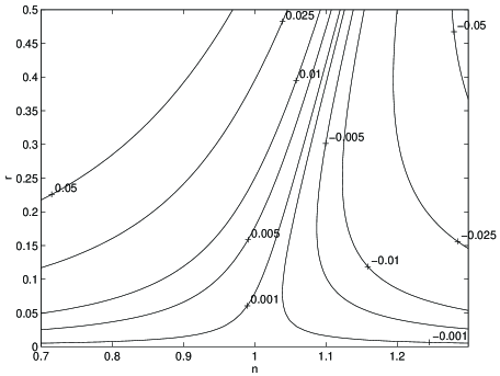
Figure 1: This shows contours of constant $dn/d\ln k$, assuming $\xi^{2}=0$. Detection of the scale dependence at 95% confidence requires roughly $|dn/d\ln k|\ga 0.01$.

As we confirmed in Section 2, gravitational waves are only detectable (at 95% confidence level) if $r_{{\rm ts}}\ga 0.1$ even if cosmic microwave background polarization is measured [Zaldarriaga et al. 1997]. The most optimistic scenario for measuring the scale dependence is if we can assume that all higher derivatives are negligible, and then with polarization a 95% confidence detection is possible if $|dn/d\ln k|\ga 0.01$. Studying the first term of Eq. (18), we immediately see that for it to be important then the tensors have to be detectable, by some margin. Much more interesting is the second term, because provided $n$ is not too close to unity, it can give a detectable contribution to the scale dependence even if $r$ is not itself detectable (though $r_{{\rm ts}}$ cannot be very small). This is illustrated in Fig. 1; there exist regions where $|dn/d\ln k|>0.01$ but where $r_{{\rm ts}}<0.1$. In fact, hybrid inflation models often have undetectable $r_{{\rm ts}}$ but $n$ significantly different from unity. The final $\xi^{2}$ term in Eq. (18) is in general independent of the others and so nothing can be said directly, other than that a priori it is as likely to reinforce the scale dependence as partially cancel it.

In conclusion, then, there exist significant parameter regions, including ones currently observationally viable, where the scale dependence of the spectral index can be measured. In such cases, it provides extra information concerning the inflation model which would not otherwise be available. In some cases, the scale dependence is measurable even when the tensor contribution is not.

4 Specific hybrid inflation models

We end with a brief description of a particular type of inflation model where $dn/d\ln k$ is detectable. Stewart [Stewart 1997a, Stewart 1997b] has recently presented two interesting models, the idea being to use quantum corrections to flatten the potential of the inflaton sufficiently to allow it to support an inflationary epoch. The argument is not difficult to reproduce. Typical inflation models require a non-zero scalar potential energy $V=V_{0}$. In supergravity this induces soft supersymmetry-breaking masses for all scalar fields leading to a classical potential:

$$V=V_{0}\left[1-{1\over 2}A\phi^{2}+...\right]$$ (19)

with $|A|\sim 1$. (Here the stringy Planck mass $M_{{\rm Pl}}\equiv m_{{\rm Pl}}/\sqrt{8\pi}$ has been set equal to one.) Unfortunately this does not lead to slow-roll inflation, since $|V^{\prime\prime}/V|\simeq|A|\sim 1$. Stewart pointed out that if $\phi$ has either gauge or Yukawa couplings, to vector or chiral superfields with soft supersymmetry breaking masses squared of order $V_{0}$, then quantum corrections will renormalize the mass of $\phi$ leading to a one-loop renormalization group effective potential of the form

$$V=V_{0}\left[1-{1\over 2}f(\delta\ln\phi)\phi^{2}+...\right]$$ (20)

where $\delta\ll 1$ is the one–loop suppression factor, $f(0)=A+O(\delta)$, with the expression being valid for $V_{0}\ll\phi^{2}\ll 1$. Such a correction can lead to slow–roll inflation in certain regions of the potential. In particular, if $\phi_{*}$ is defined by

$$f_{*}+{\delta\over 2}f^{\prime}_{*}=0$$ (21)

where $f_{*}=f(\delta\ln\phi_{*})$ and $f^{\prime}_{*}(x)=df_{*}/dx$ then $|V^{\prime\prime}/V|\sim O(\delta)$ in the vicinity around $\phi_{*}$ and the loop-corrected potential is flat enough to drive inflation even though the bare potential is not. The mechanism can work for $f^{\prime}_{*}$ either positive or negative. If it is less than zero then $\phi_{*}$ is a minimum of the potential and so a hybrid inflation mechanism is required to end inflation at some critical value $\phi_{{\rm c}}$; such a model is constructed in Stewart’s second paper [Stewart 1997b]. If $f^{\prime}_{*}>0$ then $\phi_{*}$ is a maximum of the potential. Stewart [Stewart 1997a] considered such a model where $\phi$ rolled towards the true vacuum at $\phi\sim 1$.

We are interested in the spectral index obtained and its slope. Introducing $g(y)\equiv-f_{*}(x)-\delta/2f^{\prime}_{*}(x)$ where $y\equiv\delta\ln(\phi_{*}/\phi)$ and defining $\delta$ by $\delta\ln\phi_{*}=-1$, Stewart showed that, to lowest order in the slow-roll approximation, the spectral index $n$ was given by

$$n = 1-2g^{\prime}_{*}\delta+8(1+A)\left(1-{1\over\sqrt{1+3/4(1+A)}}\right)\times$$ (22)

$$\exp\left[-2+{1\over\sqrt{1+3/4(1+A)}}-g^{\prime}_{*}\delta(N-N_{\rm fr})\right]\,,$$

where $g^{\prime}_{*}=2(1+A)/(A+\sqrt{A(A+1)}\,)$, $N-N_{\rm fr}$ is the number of $e$-folds of inflation from when the scale $k\propto e^{-N}$ leaves the horizon to $\phi=\phi_{\rm fr}$, the value of $\phi$ when it begins to fast-roll down the potential and inflation comes to an end. Since $d/d\ln k\simeq-d/dN$, it follows from Eq. (22) that

$${dn\over d\ln k} = 8(1+A)\left(1-{1\over\sqrt{1+3/4(1+A)}}\right)\times$$

$$g^{\prime}_{*}\delta\exp\left[-2+{1\over\sqrt{1+3/4(1+A)}}-g^{\prime}_{*}\delta(N-N_{{\rm fr}})\right]\,.$$

Typically the number of $e$-folds of inflation remaining after observable scales leave the horizon is 40 to 60, depending on the energy scale and the reheating efficiency. However, this may be reduced by 10 or 20 if there is a second, low-energy period of inflation known as thermal inflation [Lyth & Stewart 1995]. Low values of $N-N_{{\rm fr}}$ favour detectable scale dependence.

The most natural scale for such a particle physics motivated potential is $V_{0}\sim M_{{\rm SUSY}}^{4}$ where $M_{{\rm SUSY}}$ is the supersymmetry breaking scale in our vacuum. A value $M_{{\rm SUSY}}\sim 10^{10}$–$10^{11}$ GeV corresponds to a gravity-mediated supersymmetry breaking. The corresponding COBE normalized value of $\phi_{*}$ gives $\phi_{*}\sim 10^{-11}$, hence $\delta\sim 0.04$, a number consistent with that derived from a gauge coupling strength similar to that of the Grand Unified Theory gauge coupling inferred from LEP data, $\alpha_{{\rm GUT}}\sim 0.04$ [Stewart 1997b]. However, there is significant flexibility in the allowed values of $A$ and $V_{0}$, and hence $\delta$. A few values are tabulated in Table 2 to give a feel for the possibilities. What is encouraging is that provided there is a low number of $e$-foldings, the scale dependence can be detected by Planck or similar.

Table 2: Values of $n$ and $dn/d\ln k$ in different regions of parameter space.

$A$	$\delta$	$e$-folds	$n$	$dn/d\ln k$
1	0.02	20	1.32	0.013
1	0.02	40	1.13	0.007
1	0.04	20	1.07	0.013
1	0.04	40	0.92	0.003
2	0.02	20	1.44	0.013
2	0.02	40	1.23	0.008
2	0.04	20	1.18	0.015
2	0.04	40	0.99	0.005

5 Conclusions

We have considered the likely magnitude and impact of scale dependence of the spectral index in inflationary cosmologies. We have estimated the magnitude necessary to make the scale dependence detectable, and shown that slow-roll models of inflation, especially those of the hybrid inflation type, may give an observable effect. If so, this provides extra information on the inflaton potential which would not otherwise be available.

If scale dependence of $n$ is considered, then there is a scale (around $k_{0}\sim 0.05$ Mpc^-1) at which the uncertainty in the determination of $n$ is unchanged from the case of a power-law spectrum when the first derivative of $n$ is introduced. We find negligible degradation of the error on $n$ even when a second derivative is introduced, and have determined the anticipated errors on the first two derivatives of $n$ at the preferred scale. We have found that at other scales the errors on $n$ are significantly greater; up to a factor of around 10 greater for scales corresponding to the current horizon.

The introduction of extra parameters to model the cosmology implies that all the cosmological parameters will be more poorly determined. Fortunately, we have shown that the degradation of the uncertainty in these parameters is a small effect when the two derivatives are introduced.

References

- [Barrow & Liddle 1993] Barrow J. D., Liddle A. R., 1993, Phys. Rev. D, 47, R5129
- [Bond 1996] Bond J. R., 1996, in Schaeffer R., Silk J., Spiro M., Zinn-Justin J., eds, Cosmology and Large Scale Structure, Elsevier Science, Netherlands
- [Bond et al. 1997] Bond J. R., Efstathiou G., Tegmark M., 1997, MNRAS, 291, L33
- [Bond, Jaffe & Knox 1998] Bond J. R., Jaffe A. H., Knox L., 1998, Phys. Rev. D, 57, 2117
- [Copeland et al. 1993] Copeland E. J., Kolb E. W., Liddle A. R., Lidsey J. E., 1993, Phys. Rev. D, 48, 2529
- [Copeland et al. 1994a] Copeland E. J., Kolb E. W., Liddle A. R., Lidsey J. E., 1994a, Phys. Rev. D, 49, 1840
- [Copeland et al. 1994b] Copeland E. J., Liddle A. R., Lyth D. H., Stewart E. D., Wands D., 1994b, Phys. Rev. D, 49, 6410
- [Hodges & Blumenthal 1990] Hodges H. M., Blumenthal G. R., 1990, Phys. Rev. D, 42, 3329
- [Hodges et al. 1990] Hodges H. M., Blumenthal G. R., Kofman L. A., Primack J. R., 1990, Nucl. Phys., B335, 197
- [Jungman et al. 1996a] Jungman G., Kamionkowski M., Kosowsky A., Spergel D. N., 1996a, Phys. Rev. Lett, 76, 1007
- [Jungman et al. 1996b] Jungman G., Kamionkowski M., Kosowsky A., Spergel D. N., 1996b, Phys. Rev. D, 54, 1332
- [Kofman & Linde 1987] Kofman L. A., Linde A. D., 1987, Nucl. Phys., B282, 555
- [Kosowsky & Turner 1995] Kosowsky A., Turner M. S., 1995, Phys. Rev. D, 52, 1739
- [Liddle & Lyth 1992] Liddle A. R., Lyth D. H., 1992, Phys. Lett. B, 291, 391
- [Liddle & Lyth 1993] Liddle A. R., Lyth D. H., 1993, Phys. Rep., 231, 1
- [Liddle et al. 1994] Liddle A. R., Parsons P., Barrow J. D., 1994, Phys. Rev. D, 50, 7222
- [Lidsey et al. 1997] Lidsey J. E., Liddle A. R., Kolb E. W., Copeland E. J., Barreiro T., Abney M., 1997, Rev. Mod. Phys., 69, 373
- [Linde 1991] Linde A. D., 1991, Phys. Lett. B, 259, 38
- [Linde 1994] Linde A. D., 1994, Phys. Rev. D, 49, 748
- [Lyth 1996] Lyth D. H., 1996, Lancaster preprint hep-ph/9609431
- [Lyth 1997] Lyth D. H., 1997, Phys. Rev. Lett, 78, 1861
- [Lyth & Stewart 1995] Lyth D. H., Stewart E. D., 1995, Phys. Rev. Lett., 75, 201
- [Magueijo & Hobson 1997] Magueijo J., Hobson M. P., 1997, Phys. Rev. D, 56, 1908
- [Salopek et al. 1989] Salopek D. S., Bond J. R., Bardeen J. M., 1989, Phys. Rev. D, 40, 1753
- [Seljak & Zaldarriaga 1996] Seljak U., Zaldarriaga M., 1996, ApJ, 469, 437
- [Stewart 1997a] Stewart E. D., 1997a, Phys. Lett. B, 391, 34
- [Stewart 1997b] Stewart E. D., 1997b, Phys. Rev. D, 56, 2019
- [Tegmark 1997] Tegmark M., 1997, Phys. Rev. D, 55, 5895
- [Tegmark et al. 1997] Tegmark M., Taylor A. N., Heavens A. F., 1997, ApJ, 480, 22
- [Zaldarriaga et al. 1998] Zaldarriaga M., Seljak U., Bertschinger E., 1998, ApJ, 494, 491
- [Zaldarriaga et al. 1997] Zaldarriaga M., Spergel D. N., Seljak U., 1997, ApJ, 488, 1