Redshift Space Distortions of the Correlation Function in Wide Angle Galaxy Surveys

Abstract

Using a novel two-dimensional coordinate system, we have derived a particularly simple way to express the redshift distortions in galaxy redshift surveys with arbitrary geometry in closed form. This method provides an almost ideal way to measure the value of $\beta=\Omega_{0}^{0.6}/b$ in wide area surveys, since all pairs in the survey can be used for the analysis. In the limit of small angles, this result straightforwardly reduces to the plane-parallel approximation. This expansion can also be used together with more sophisticated methods such as for the calculation of Karhunen-Loeve eigenvectors in redshift space for an arbitrary survey geometry. Therefore, these results should provide for more precise methods in which to measure the large scale power spectrum and the value of $\beta$ simultaneously.

1 Introduction

The fact that the correlation function in redshift space is distorted from the real space correlations is well known. Davis and Peebles (1983) have demonstrated quantitatively that the correlation function $\xi(\pi,\sigma)$, expressed as a function of the line-of-sight $(\pi)$ and perpendicular $(\sigma)$ separations, has a significant anisotropy. By measuring the elongation of this function along the $(\pi)$ axis, a value of the one-dimensional velocity dispersion can be inferred. They found that the velocity distribution was well described by an exponential distribution and that the value of the dispersion was relatively independent of scale, at around 350 km/s. Peebles (1980) gives a nice summary why in linear theory the typical velocities of the galaxies scale with $\Omega_{0}^{0.6}$. With the advent of biased galaxy formation (Bardeen et al 1986), the velocities have been rescaled by a bias factor $b$, leading to velocities dependent upon the combination $\beta=\Omega^{0.6}/b$.

In Kaiser’s (1987) pioneering work, the effect of the infall due to linear theory was identified and it was shown that in the limit that the lines of sight to the two galaxies are approximately parallel to each other, the power spectrum $P(k)$ is enhanced as a function of the directional cosine $\mu$ between the wave vector and the line-of-sight as

$$P^{s}(k,\mu)=P(k)(1+\beta\mu^{2})^{2}.$$ (1)

In related work, Lilje and Efstathiou(1989) calculated the angular average of the redshift correlation function directly related to this expression. Hamilton(1992) expanded the redshift space correlation function into components, multiplied with the angular multipoles. He showed that only the quadrupole and hexadecapole terms arise in linear theory, in agreement with Kaiser’s expression. Other promising approaches have involved an expansion into orthogonal eigenfunctions (Heavens and Taylor 1994), or restricting the surveys to small opening angles so that the plane-parallel approximation still holds (Cole, Fisher and Weinberg 1994,1995). These papers attempted to measure the parameter $\beta$ from the quadrupole to monopole ratio.

Zaroubi and Hoffmann (1996) outlined how to compute a linear expansion of the redshift space correlation function for a general geometrical configuration and provided numerical estimates of the redshift distortions. Additionally, Hamilton and Culhane (1996), hereafter HC96, have introduced a novel integral transform, rotationally invariant and commuting with the redshift distortion operator, which makes the transformation very elegant and simple.

Here we present simple and intuitive expressions to calculate the redshift distortions which exploit the fact that the inherent geometry of the problem is two dimensional. Indeed, by rotating all pairs in a redshift survey to a common plane and analyzing the redshift distortions in that plane, we obtain particularly simple analytic results. These results smoothly approach the Kaiser/Hamilton plane-parallel limit in which angle between the galaxy pair in a survey is small. Additionally, these expressions allow for a much more productive use of redshift surveys since all galaxy pairs can be utilized in a given wide angle survey. It can also be used in adjunct with more sophisticated methods of analysis such as construction of eigenvectors for a KL analysis (Vogeley and Szalay 1996).

2 The Correlation Function in Redshift Space

2.1 The Coordinate System

The symmetries in the geometric configuration of redshift surveys have been elegantly described in HC96, who recognized that the correlation function in redshift space is tied to a triangle formed by the observer and the two galaxies which lie upon two arbitrary lines of sight. The correlation function should be a function of this triangle, but otherwise invariant under rotations about the observer. Such invariant triangles can be characterized by one size and two shape parameters. We will use two angles to describe the shape of the triangle, and express the scale dependence of the correlation function as a function of $r=|{\bf r}|$, the distance between the two points.

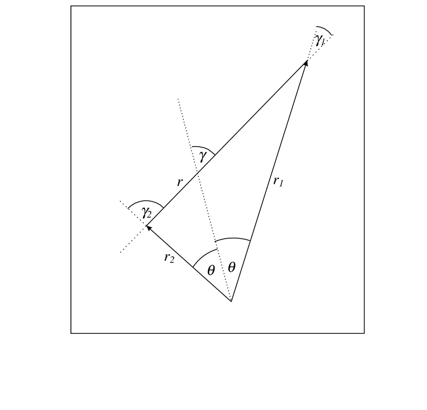
Figure 1: A graphic representation of our coordinate system. The angle between the two lines of sight is $2\theta$. The main line-of-sight is taken to be the axis bisecting the angle $2\theta$, since this is the symmetry axis for the two directions ${\hat{\bf r}}_{1}$ and ${\hat{\bf r}}_{2}$. The angle $\gamma$ is defined by the main line of sight and the vector ${\bf r}$.

In this coordinate system, which is illustrated in Fig. 1, the two points are located at points ${\bf r}_{1}=r_{1}{\hat{\bf r}}_{1}$ and ${\bf r}_{2}=r_{2}{\hat{\bf r}}_{2}$. The observer is at the origin, at rest in comoving frame. The angle between the two normal vectors is $2\theta$, that is ${\hat{\bf r}}_{1}{\hat{\bf r}}_{2}=\cos 2\theta$. The separation between the two points is ${\bf r}={\bf r}_{1}-{\bf r}_{2}$, with a normal vector ${\hat{\bf r}}$. The angles between ${\hat{\bf r}}_{1},{\hat{\bf r}}_{2}$ and ${\hat{\bf r}}$ are $\gamma_{1}$ and $\gamma_{2}$ respectively. The symmetry axis for ${\hat{\bf r}}_{1}$ and ${\hat{\bf r}}_{2}$ is found by halving the angle $2\theta$. The angle between this symmetry axis and ${\bf r}$ is $\gamma$. We assume that $r_{1}>r_{2}$, thus $\gamma_{2}>\gamma_{1}$. The angles are related to each other as $\gamma_{1}+\gamma_{2}=2\gamma$, and $\gamma_{2}-\gamma_{1}=2\theta$. This introduction implies our choice of the two angles, $\gamma$ and $\theta$, which together with $|{\bf r}|$ completely describe the shape of the triangle. These angles are particularly convenient since $\theta$ is given by our geometry and $\gamma$ smoothly approaches the angle familiar in the plane-parallel limit as $\theta$ tends to 0. There is another geometric relation between the two angles: if $\theta$ is not 0, then the smallest value $\gamma$ can take is $\theta$, and its largest value is $\pi-\theta$. This is not due to the choice of coordinates but rather to the geometry of the problem.

We will provide an expression for the distortions of the correlation function as a series expansion in terms of the angle $\gamma$, where the coefficients have a simple $r$ and $\theta$ dependence, together with a dependence on the parameter $\beta$ that we wish to measure. So far our approach has been quite similar to most earlier work except for the introduction of a convenient set of angles which will simplify the results considerably.

It has been a persistent problem to get a simple power spectrum or correlation function beyond the Kaiser (1987) plane-parallel limit. The difficulty lies in that the Fourier space transfer function, the ratio of the distorted and undistorted power spectrum contains a strong mode-coupling (Zaroubi and Hoffmann 1996). Thus, the transfer function is not multiplicative but contains an integral over a non-local kernel with a strong $k$-dependence. This dependence strongly affects the multipole coefficients which would otherwise make a precise determination of $\beta$ quite straightforward. One alternative has been to use only galaxy pairs at small angular separations (e.g. Cole et al 1994, 1995).

It is interesting to consider what the reasons are for this non-locality. With a finite $\theta$, the original symmetry of the problem is lost, and the geometry is inherently two-dimensional. This effect is thus arising from ‘aliasing’ (Kaiser and Peacock 1991, Szalay et al 1993, Landy et al 1996), i.e. projections of the spherically isotropic power to the lower dimensions of the survey geometry. Interestingly enough, even though the power spectrum is definitely non-local, the redshift space correlation function can still be computed in spherical coordinates, and it can be expressed in a closed form, as will be shown below.

In the following Section 2.2, we will first derive a representation of the redshift distortion problem in terms of spherical tensors. This development, being a representation independent expansion, is independent of our choice of coordinate system described above. In Section 2.3, we will reintroduce our coordinates and show how the coefficients of this expansion can be most economically expressed using these coordinates.

2.2 Expansion in Spherical Tensors

We can assume without a loss of generality, that the observer is at rest with respect to the CMB frame. As shown by HC96, this effect can be trivially included. The linear expansion of the overdensity at a redshift space coordinate ${\bf s}$ relates to the real-space overdensity at ${\bf r}$, with ${\bf s}={\bf r}+u{\hat{\bf r}}$, as a function of the radial velocity $u$ and its line-of-sight derivative $\partial u/\partial r$, as first introduced by Kaiser (1987),

$$\delta^{(s)}({\bf r})=\delta^{(r)}({\bf r})-\frac{\partial u({\bf r})}{\partial r}-\alpha(r)u({\bf r}),$$ (2)

Here $\alpha(r)=(2+\partial\ln\phi(r)/\partial\ln r)/r$, where $\phi(r)$ is the selection function which is a slowly varying function of $r$, the radial distance from the observer. Due to the fact that the velocity scale is much smaller than the typical depth of todays redshift surveys, this term is very small and is generally ignored. We will include this term for completeness in our results but would like to make one other point why this term is additionally small. If the redshift survey is defined by a boundary on the sky, a given selection function, and a range of the radial coordinate $(a,b)$, then $\alpha$ will be averaged, weighted by the selection function. Integrating by parts one can show that this term is small and becomes zero as the lower limit becomes 0 and the upper limit $\infty$, the case of full surveys.

The peculiar velocity can be written concisely as a Fourier integral, with the usual $\beta=\Omega_{0}^{0.6}/b$, as

$$u({\bf r})=i\beta\int\kern-2.5pt{d^{3}k\over(2\pi)^{3}}\,\frac{{\hat{\bf k}}{\hat{\bf r}}}{k}e^{i{\bf k}{\bf r}}\tilde{\delta}({\bf k}).$$ (3)

In order to simplify subsequent calculations, we introduce here the spherical tensor $A$ as

$$A_{l}^{n}({\bf r})=\int\kern-2.5pt{d^{3}k\over(2\pi)^{3}}\,(ik)^{-n}P_{l}({\hat{\bf k}}{\hat{\bf r}})e^{i{\bf k}{\bf r}}\tilde{\delta}({\bf k}).$$ (4)

One can then reexpress the redshift-space overdensity at the point ${\bf r}$ in terms of $A$ as

$$\delta^{(s)}({\bf r})=\left(1+\frac{\beta}{3}\right)A_{0}^{0}({\bf r})+\frac{2}{3}\beta A_{2}^{0}({\bf r})+\beta\alpha(r)A_{1}^{1}({\bf r}).$$ (5)

This use of spherical coordinates makes it easy to express the correlation of the different $A$ components, at positions ${\bf r}_{1}$ and ${\bf r}_{2}$ as

$$S_{l_{1}l_{2}}^{n_{1}+n_{2}}=\left\langle A_{l_{1}}^{n_{1}}({\bf r}_{1})A_{l_{2}}^{n_{2}}({\bf r}_{2})\right\rangle=(-1)^{l_{2}}\int\kern-2.5pt{d^{3}k\over(2\pi)^{3}}\,(ik)^{-(n_{1}+n_{2})}P_{l_{1}}({\hat{\bf k}}{\hat{\bf r}}_{1})P_{l_{2}}({\hat{\bf k}}{\hat{\bf r}}_{2})e^{i{\bf k}{\bf r}}P(k).$$ (6)

where $P_{l}$ is the Legendre polynomial, ${\bf r}={\bf r}_{1}-{\bf r}_{2}$ and $P(k)$ is the power spectrum with the definition $\left\langle\tilde{\delta}({\bf k})\tilde{\delta}({\bf k}^{\prime})\right\rangle=(2\pi)^{3}\delta^{3}({\bf k}+{\bf k}^{\prime})P(k)$. The redshift-space two-point correlation function of finite-angle is given in terms of $S_{l_{1}l_{2}}^{n}$, where we will use $\alpha_{i}=\alpha(r_{i})$.

$$\xi^{(s)}({\bf r}_{1},{\bf r}_{2}) \!\!\!= \!\!\!\left(1+\frac{\beta}{3}\right)^{2}S_{00}^{0}+\frac{4}{9}\beta^{2}S_{22}^{0}+\frac{2}{3}\beta\left(1+\frac{\beta}{3}\right)\left(S_{02}^{0}+S_{20}^{0}\right)$$ (7)

$$+\, \beta\left(1+\frac{\beta}{3}\right)\left[\alpha_{1}S_{10}^{1}+\alpha_{2}S_{01}^{1}\right]+\frac{2}{3}\beta^{2}\left[\alpha_{1}S_{12}^{1}+\alpha_{2}S_{21}^{1}\right]-\,\beta^{2}\alpha_{1}\alpha_{2}S_{11}^{2}$$

Both the Legendre polynomials and the plane wave $e^{i{\bf k}{\bf r}}$ can be expanded in terms of spherical harmonics as

$$P_{l}({\hat{\bf k}}{\hat{\bf r}}) \!\!\!= \!\!\!\frac{4\pi}{{2l\kern-1.99997pt+\kern-1.99997pt1}}\sum_{m=-l}^{l}Y_{lm}^{*}({\hat{\bf k}})Y_{lm}({\hat{\bf r}}),$$ (8)

$$e^{i{\bf k}{\bf r}} \!\!\!= \!\!\!4\pi\sum_{l=0}^{\infty}\sum_{m=-l}^{l}i^{l}j_{l}(kr)Y_{lm}^{*}({\hat{\bf k}})Y_{lm}({\hat{\bf r}}),$$ (9)

where $j_{l}$ and $Y_{lm}$ are spherical Bessel functions and spherical harmonics, respectively. We can express the integral of three $Y_{lm}$’s over $d{\mit\Omega}_{\bf k}$ with the Wigner $3j$-symbols. We also introduce the bipolar spherical harmonics $X^{LM}_{l_{1}l_{2}}({\hat{\bf r}}_{1},{\hat{\bf r}}_{2})$ which transform as a spherical harmonic with $L,M$ with respect to rotations (Varshalovich et al 1988).

$$X^{LM}_{l_{1}l_{2}}({\hat{\bf r}}_{1},{\hat{\bf r}}_{2})=(-1)^{l_{1}-l_{2}-M}\sqrt{{2L\kern-1.99997pt+\kern-1.99997pt1}}\sum_{m_{1},m_{2}}\left(\begin{array}[]{ccc}l_{1}&l_{2}&L\\ m_{1}&m_{2}&-M\end{array}\right)Y_{l_{1}m_{1}}({\hat{\bf r}}_{1})Y_{l_{2}m_{2}}({\hat{\bf r}}_{2})$$ (10)

With $Y_{LM}({\hat{\bf r}})$ these can form a rotationally invariant scalar, dependent on $L,l_{1},l_{2}$, where $\Delta$ indicates the shape of the triangle formed by the three unit vectors. Any quantity that is a scalar function of $\Delta$ is independent of what angles or parameters we may choose to describe the triangle shape. This invariant scalar $B$ is symmetric in $l_{1},l_{2}$.

$$B^{L}_{l_{1}l_{2}}(\Delta)={1\over\sqrt{({2l_{1}\kern-1.99997pt+\kern-1.99997pt1})({2l_{2}\kern-1.99997pt+\kern-1.99997pt1})}}\left(\begin{array}[]{ccc}l_{1}&l_{2}&L\\ 0&0&0\end{array}\right)\sum_{M}X^{LM*}_{l_{1}l_{2}}({\hat{\bf r}}_{1},{\hat{\bf r}}_{2})Y_{LM}({\hat{\bf r}}).$$ (11)

With this notation, equation (6) reduces to

$$S_{l_{1}l_{2}}^{n}=(4\pi)^{3/2}(-1)^{l_{1}}\sum_{L}i^{L-n}B^{L}_{l_{1}l_{2}}(\Delta)\,\xi_{L}^{(n)}(r)$$ (12)

where

$$\xi_{L}^{(n)}(r)=\frac{1}{2\pi^{2}}\int dk\,k^{2}k^{-n}j_{L}(kr)P(k),$$ (13)

2.3 Expansion of the Correlation Function

The above expression shows the correlation function can be written in terms of a series, factorized into size $r$ and shape $\Delta$ dependent terms, providing a representation independent expansion. Equations (7) and (12) give an expression of the redshift-space correlation function. Re-expanding in terms of $\xi^{(n)}_{L}(r)$, the $\Delta$ dependence is contained in the coefficients $c_{ij}(\Delta)$:

$$\xi^{(s)}(r,\Delta)=c_{00}\xi^{(0)}_{0}+c_{02}\xi^{(0)}_{2}+c_{04}\xi^{(0)}_{4}+c_{11}\xi^{(1)}_{1}+\,c_{13}\xi^{(1)}_{3}+c_{20}\xi^{(2)}_{0}+c_{22}\xi^{(2)}_{2},$$ (14)

It is at this point that the use of any particular coordinate system becomes paramount. Since the coefficients $c_{ij}(\Delta)$ are functions of the shape of the triangle under consideration, a judicious use of coordinates can simplify the problem considerably, as will be shown below. The terms proportional to $\sin^{2}(\theta)$ have been saparated, since these disappear in the plane-parallel limit. After a somewhat tedious reduction procedure, most of it carried out in Mathematica, we obtain the following results:

$$c_{00} \!\!\!= \!\!\!1+\frac{2}{3}\beta+\frac{1}{5}\beta^{2}-\frac{4}{15}\beta^{2}\cos^{2}\theta\sin^{2}\theta,$$ (15)

$$c_{02} \!\!\!= \!\!\!-\left(\frac{4}{3}\beta+\frac{4}{7}\beta^{2}\right)\cos 2\theta P_{2}(\cos\gamma)-\frac{2}{3}\left(\beta-\frac{1}{7}\beta^{2}+\frac{4}{7}\beta^{2}\sin^{2}\theta\right)\sin^{2}\theta,$$ (16)

$$c_{04} \!\!\!= \!\!\!\frac{8}{35}\beta^{2}P_{4}(\cos\gamma)-\frac{4}{21}\beta^{2}\sin^{2}\theta P_{2}(\cos\gamma)-\frac{1}{5}\beta^{2}\left(\frac{4}{21}-\frac{3}{7}\sin^{2}\theta\right)\sin^{2}\theta$$ (17)

and

$$c_{11} =\,\,\, (\alpha_{1}-\alpha_{2})\left(\beta+\frac{3}{5}\beta^{2}-\frac{4}{5}\beta^{2}\sin^{2}\theta\right)\cos\theta P_{1}(\cos\gamma)$$ (18)

$$\,\,\,+ (\alpha_{1}+\alpha_{2})\left(\beta+\frac{3}{5}\beta^{2}-\frac{4}{5}\beta^{2}\cos^{2}\theta\right)\sin\theta P_{1}(\sin\gamma)$$

$$c_{13} =\,\,\, \frac{1}{5}(\alpha_{1}-\alpha_{2})\beta^{2}\cos\theta[\sin^{2}\theta P_{1}(\cos\gamma)-2P_{3}(\cos\gamma)]$$ (19)

$$\,\,\,+ \frac{1}{5}(\alpha_{1}+\alpha_{2})\beta^{2}\sin\theta[\cos^{2}\theta P_{1}(\sin\gamma)-2P_{3}(\sin\gamma)]$$

$$c_{20} =\,\,\, \frac{1}{9}\alpha_{1}\alpha_{2}\beta^{2}(4\cos\theta-1),$$ (20)

$$c_{22} =\,\,\, \frac{1}{3}\alpha_{1}\alpha_{2}\beta^{2}\sin^{2}\theta-\frac{2}{3}\alpha_{1}\alpha_{2}\beta^{2}P_{2}(\cos\gamma).$$ (21)

The first set of coefficients, which do not contain $\alpha$, capture most of the relevant physics. For the sake of completeness, the second set gives the $\alpha$-dependent terms $c_{11}$, $c_{13}$, $c_{20}$ and $c_{22}$ which must be included for calculations in which $\alpha_{1}$ and $\alpha_{2}$ cannot be neglected.

From these expressions, it is evident that a good choice of coordinate system matters a great deal. Using the system discussed above (angles $\theta$ and $\gamma$, separation $r$), leads to remarkably simple expressions for the coefficients $c$. Other systems we explored generally contained a lot of associated Legendre polynomials. It is easily seen in the above expression that taking the limit $\theta\rightarrow 0$ reproduces Kaiser-Hamilton’s plane-parallel result.

3 Discussion

We have presented a derivation of the redshift space correlation function between galaxies at two infinitesimal volume elements separated by an arbitrary angle, and have obtained very simple closed form analytic expressions for the correlations. These equations show that the effects of a finite angle are quite important. These are illustrated graphically in Figure 2 which indicates how the redshift distortions change as the angle between the two lines of sight is increased from 0 to 120 degrees.

Since most of the next generation redshift surveys are wide angle with the majority of pairs separated at angles greater than 10 degrees, the use of these expressions will dramatically increase the amount of information which can be extracted from the surveys resulting in more robust measurements and smaller shot noise contamination. Also, if the survey is not contiguous but consists of several slices like the Las Campanas Survey (Landy etal 1996), or the 2dF survey which will be formed from hundreds of pencilbeams, this approach can use all the data together to estimate the infall distortions.

Another promising approach to study the large scale behavior of the power spectrum is with building up a Karhunen-Loeve basis (Vogeley and Szalay 1996). The first step in that method is to subdivide the survey into small cells (in redshift space) and then construct their correlation matrix. Most pairs of cells will have a large relative angle. Thus, with the expressions presented here, computing the correlation matrix is a trivial exercise. Once the appropriate basis has been created, one can use the Fisher matrix to select the set of eigenmodes most sensitive to $\beta$, yielding an optimal estimation of the value of $\beta$.

In conclusion, we believe that our results allow a much more elegant treatment of the redshift distortions in a general geometry than before with the added benefit that all galaxy pairs may be utilized to construct a signal.

Figure 2: Contour plots of the redshift-space correlation functions in polar coordinate system $r,\gamma$ for fixed finite angles $\theta$. A standard CDM model with COBE normalization and $H_{0}=70$ km s^-1 Mpc^-1 is assumed. Plots (a), (b), (c) and (d) correspond to $\theta=0,30,45$ and $60$ degrees. Solid and dashed lines indicate positive and negative values, respectively. Contour spacings are $\Delta\log_{10}|\xi|=0.25$. Solid thick lines represent the value 100, 10, 1 and 0.1. Dashed thick lines represent the value -1 and -0.1. Blank areas correspond to unphysical regions $\gamma>\theta$.

References

- (1) Bardeen, J., Bond, J.R., Kaiser, N., Szalay, A.S. 1986, ApJ, 304,15
- (2) Cole, S., Fisher, K.B., Weinberg, D.H. 1994, MNRAS, 267, 785
- (3) Cole, S., Fisher, K.B., Weinberg, D.H. 1995, MNRAS, 275, 515
- (4) Davis, M., Peebles, P.J.E. 1983, ApJ,267, 465
- (5) Hamilton, A.J.S. 1992, ApJ, 385, L5
- (6) Hamilton, A.J.S., Culhane, M. 1996, MNRAS, 278, 73
- (7) Heavens, A.F., Taylor, A.N. 1995, MNRAS, 275, 483
- (8) Landy,S.A., Schectman,S.A., Lin,H., Kirshner,R. Oemler,A.A., Tucker,D. 1996, ApJ, 456, 1
- (9) Lilje, P., Efstathiou, G.P. 1989, MNRAS, 236, 851
- (10) Kaiser, N. 1987, MNRAS, 227, 1
- (11) Kaiser, N. and Peacock, J.A. 1991, ApJ, 379, 482
- (12) Peebles, P.J.E. 1980, The Large Scale Structure of the Universe, (Princeton University Press: Princeton)
- (13) Szalay, A.S., Broadhurst,T.J., Ellman, N., Koo, D.C., Ellis, R.S. 1993, Proc. Nat. Acad. Sci., 90, 4853
- (14) Varshalovich, D.A., Moskalev, A.N., Khershonski, V.K. 1988, Quantum Theory of Angular Momentum (World Scientific)
- (15) Vogeley, M.S. Szalay, A.S. 1996, ApJ, 465, 34
- (16) Zaroubi, S., Hoffmann, Y. 1996, ApJ, 462, 25