Textures and Cosmic Microwave Background
non–Gaussian Signatures

Abstract

We report briefly on a recent analysis of the texture–induced CMB radiation three–point correlation function of temperature anisotropies as predicted by an analytical model. We specialize our analysis to both large–scales (e.g., for COBE–DMR, where we compare our prediction with the actual four–year data) and intermediate–scales. We show how the latter case puts strong constraints on the model parameters.

Alejandro Gangui

ICTP – International Center for Theoretical Physics,
P. O. Box 586, 34100 Trieste, Italy.

1 Introduction

The anisotropies in the Cosmic Microwave Background are a powerful test for models of structure formation in the universe. The possibility of a departure from Gaussianity of the statistics of the anisotropies would disfavor standard inflation. It follows that it is interesting to calculate the predictions texture make regarding non–Gaussian signatures. It was recently proposed [1] a simple analytical model for the computation of the ${\cal C}_{\ell}$’s from textures. The model exploits the fact that in this scenario the microwave sky will show evidence of spots due to perturbations in the effective temperature of the photons resulting from the non–linear dynamics of concentrations of energy–gradients of the texture field. The model of course does not aim to replace the full range numerical simulations but just to show overall features predicted by textures in the CMB anisotropies. In fact the model leaves free a couple of parameters that are fed in from numerical simulations, like the number density of spots, $\nu$, the scaling size, $d_{s}$, and the brightness factor of the particular spot, $a_{k}$, telling us about its temperature relative to the mean sky temperature. Texture configurations giving rise to spots in the CMB are assumed to arise with a constant probability per Hubble volume and Hubble time. In an expanding universe one may compute the surface probability density of spots

$$dP=N(y)dyd\Omega,\quad\mbox{with}\quad N(y)=-{8\nu\ln(2)\over 3}\left(2^{y/3}-1\right)^{2},$$ (1.1)

where $\Omega$ stands for a solid angle on the two–sphere and the time variable $y(t)\equiv\log_{2}(t_{0}/t)$ measures how many times the Hubble radius has doubled since proper time $t$ up to now (e.g., for a redshift $z_{\rm ls}\sim 1400$ at last scattering we have $y_{\rm ls}\simeq\log_{2}[(1400)^{3/2}]\simeq 16$). In the present context the anisotropies arise from the superposition of the contribution coming from all the individual spots $S_{k}$ produced from $y_{\rm ls}$ up to now, and so, $\Delta T/T=\sum_{k}a_{k}S_{k}(\theta_{k},y)$, where the random variable $a_{k}$ stands for the brightness of the hot/cold $k$–th spot with characteristic values to be extracted from numerical simulations [2]. $S_{k}(\theta_{k},y)$ is the characteristic shape of the spots produced at time $y$, where $\theta_{k}$ is the angle in the sky measured with respect to the center of the spot. A spot appearing at time $y$ has typically a size $\theta^{s}(y)\simeq d_{s}~{}\theta^{\rm hor}(y)$, with $\theta^{\rm hor}(y)$ the angular size of the horizon at $y$, and where it follows that $\theta^{s}(y)=\arcsin\left({0.5d_{s}\over 2^{y/3}-1}\right)$. Textures are essentially causal seeds and therefore the spots induced by their dynamics cannot exceed the size of the horizon at the time of formation, hence $d_{s}\leq 1$. Furthermore the scaling hypothesis implies that the profiles satisfy $S_{k}(\theta_{k},y)=S(\theta_{k}/\theta^{s}(y))$. From all this it follows a useful expression for the multipole coefficients, $a_{\ell}^{m}=\sum_{k}a_{k}S^{\ell}_{k}(y){Y_{\ell}^{m}}^{*}(\hat{\gamma}_{k})$, with $S^{\ell}_{k}(y)$ the Legendre transform of the spot profiles. At this point the ${\cal C}_{\ell}$’s are easily calculated [1]. As we are mainly concerned with the three–point function we go on and compute the angular bispectrum predicted within this analytical model, which we find to be ($\bigl{\langle}a^{3}\bigr{\rangle}$ is the mean cubic value of the spot brightness)

$$\bigl{\langle}a_{\ell_{1}}^{m_{1}}a_{\ell_{2}}^{m_{2}}a_{\ell_{3}}^{m_{3}}\bigr{\rangle}=\bigl{\langle}a^{3}\bigr{\rangle}\int dyN(y)S^{\ell_{1}}(y)S^{\ell_{2}}(y)S^{\ell_{3}}(y)\int d\Omega_{\hat{\gamma}}Y_{\ell_{1}}^{m_{1}}(\hat{\gamma})Y_{\ell_{2}}^{m_{2}}(\hat{\gamma})Y_{\ell_{3}}^{m_{3}}(\hat{\gamma}).$$ (1.2)

Having the expression for the bispectrum we may just plug it in the formulae for the full mean three–point temperature correlation function [3]. To make contact with experiments however we restrict ourselves to the collapsed case where two out of the three legs of the three–point function collapse and only one angle, say $\alpha$, survives (this is in fact one of the cases analyzed for the four–year COBE–DMR data [4]). The collapsed three–point function thus calculated, $\bigl{\langle}C_{3}(\alpha)\bigr{\rangle}$, corresponds to the mean value expected in an ensemble of realizations. However, as we can observe just one particular realization, we have to take into account the spread of the distribution of the three–point function values when comparing a model prediction with the observational results. This is the well–known cosmic variance problem. We can estimate the range of expected values about the mean by the rms dispersion $\sigma_{CV}^{2}(\alpha)\equiv\bigl{\langle}C_{3}^{2}(\alpha)\bigr{\rangle}-\bigl{\langle}C_{3}(\alpha)\bigr{\rangle}^{2}$. We will estimate the range for the amplitude of the three–point correlation function predicted by the model by $\bigl{\langle}C_{3}(\alpha)\bigr{\rangle}\pm\sigma_{CV}(\alpha)$. It has been shown [2] that spots generated from random field configurations of concentrations of energy gradients lead to peak anisotropies 20 to 40% smaller than those predicted by the spherically symmetric self–similar texture solution. These studies also suggest an asymmetry between maxima $\langle a_{\rm max}\rangle$ and minima $\langle a_{\rm min}\rangle$ of the peaks as being due to the fact that, for unwinding events, the minima are generated earlier in the evolution (photons climbing out of the collapsing texture) than the maxima (photons falling in the collapsing texture), and thus the field correlations are stronger for the maxima, which enhance the anisotropies.

2 Comparison with observations

Let us now compute the predictions on the CMB non–Gaussian features derived from the present analytical texture model. One needs to have the distribution of the spot brightness $\{a_{k}\}$ in order to compute the mean values $\langle a^{n}\rangle$. It is enough for our present purposes to take for all hot spots the same $a_{h}>0$ and for all the cold spots the same $a_{c}<0$. Then the $\langle a^{n}\rangle$ needed can readily be obtained in terms of $\langle a^{2}\rangle$ and $x\equiv\langle a\rangle/\langle|a|\rangle$. We fix $\langle a^{2}\rangle$ from the amplitude of the anisotropies according to four–year COBE–DMR [4]. The other parameter, $x$, that measures the possible asymmetry between hot and cold spots, we leave as a free parameter. We first consider the COBE–DMR window function and, in order to take into account the partial sky coverage due to the cut in the maps at Galactic latitudes $|b|<20^{\circ}$, we multiply $\sigma_{CV}$ by a factor $\sim 1.5$ in the numerical results (sample variance). Let us now compare with the data: Subtracting the dipole and for all reasonable values of the asymmetry parameter $x$, the data falls well within the $\bigl{\langle}C_{3}(\alpha)\bigr{\rangle}\pm\sigma_{CV}(\alpha)$ band, and thus there is good agreement with the observations. However, the band for Gaussian distributed fluctuations (e.g., as predicted by inflation) also encompasses the data well enough, and it is in turn included inside the texture predicted band. This makes it impossible to draw conclusions favoring one of the models [5].

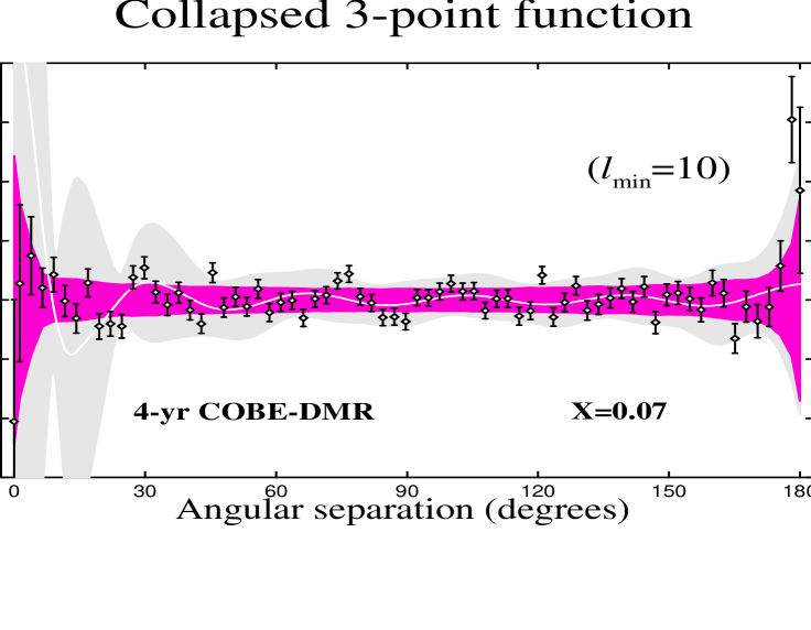
Figure 1: The collapsed three–point function (white curve) and the rms cosmic variance (grey band) which includes also the $\sim 50\%$ increment due to the sample variance, in units of $10^{4}{\mu}{\rm K}^{3}$, as predicted by the analytical texture model. The asymmetry parameter is $x=0.07$, as suggested by simulations. Also shown is the ‘pseudo–collapsed’ three–point function as computed from the analysis of the four–year COBE–DMR data. Error bars represent instrument noise while the dark band represents the rms range of fluctuations due to a superposition of instrument noise and cosmic and sample variance.

It is well known that the largest contribution to the cosmic variance comes from the small values of $\ell$. Thus, the situation may improve if one subtracts the lower order multipoles contribution, as in a $\ell_{min}=10$ analysis [6]. In Figure 1 we show the analysis of the four–year COBE–DMR data evaluated from the 53 + 90 GHz combined map, containing power from the $\ell=10$ moment and up. It is apparent that the fluctuations about zero correlation (i.e., no signal) are too large for the instrument noise to be the only responsible. These are however consistent with the range of fluctuations expected from a Gaussian process (dark band). What we want to see now is whether our analytical texture model for the three–point function [5] can do better when compared with the data. In the same figure we show the collapsed three–point function $\bigl{\langle}C_{3}(\alpha)\bigr{\rangle}$ (white curve) and the grey band indicates the rms range of fluctuations expected from the cosmic variance. From this figure one may see qualitatively by eye that (for some ranges of the angular separation better than for others, of course) the data seems to follow ‘approximately’ the trend of the texture curves.

An experiment probing smaller angular scales than COBE should thus be more appropriate to test non–Gaussian features in texture models. As an example we compute the predictions for a three–beam subtraction scheme experiment with window function at zero–lag ${\cal W}_{\ell}=(1.5-2P_{\ell}(\cos\theta)+0.5P_{\ell}(\cos 2\theta))^{1/2}\exp(-\ell(\ell+1)\sigma^{2}/2)$, where $\sigma=0.64^{\circ}$ is the beam width and $\theta=2.57^{\circ}$ is the chopping angle. This window function is peaked at $\ell\sim 70$ and the range of multipoles that significantly contribute to the three–point function is from $\ell=10$ to $\ell=100$. Hence we are still probing large enough scales and our results are not strongly affected by the microphysics of the last scattering surface. We obtain for the skewness $S\equiv\langle C_{3}(0)\rangle=(4.75\pm 1.94)\times 10^{4}\mu{\rm K}^{3}$, where the error band stands for the associated cosmic variance $\sigma_{CV}^{2}(0)$, for a value of $x=0.07$. For comparison, the Gaussian adiabatic prediction is $S_{\rm Gauss}=0.06\times 10^{4}\mu{\rm K}^{3}$. Thus, in this case even for reasonably small values of the asymmetry parameter $x$ one such experiment can in principle distinguish between inflation and texture predictions, and thus put stronger constraints on the model parameters.

Acknowledgments: I thank Silvia Mollerach for her collaboration in this work, and Gary Hinshaw for the courtesy of providing the 4-yr data, Ruth Durrer, David Wands for instructive conversations during these journées, and the organizers for their invitation to present our work. I acknowledge partial funding from The British Council/Fundación Antorchas, and thank Dennis Sciama for his continuous support.

References

- [1] J. Magueijo, Phys. Rev. D 52, 689 (1995).
- [2] J. Borrill et al., Phys. Rev. D. 50, 2469 (1994).
- [3] A. Gangui, F. Lucchin, S. Matarrese and S. Mollerach, Astrophys. J. 430, 447 (1994).
- [4] E. W. Wright et al., Astrophys. J. 464, L21 (1996).
- [5] A. Gangui and S. Mollerach, Phys. Rev. D 54, 4750 (1996).
- [6] G. Hinshaw et al., Astrophys. J. 446, L67 (1995).