SEARCH FOR EXTRA-SOLAR PLANETS THROUGH MONITORING MICROLENSING EVENTS FROM ANTARCTICA

Abstract

During the months when the galactic bulge is visible from the southern hemisphere, there are typically about 8 to 10 on-going microlensing events at any given time. If the lensing stars have planets around them, then the signature of the planets can be seen as sharp, extra peaks on the microlensing light curves. And if every lensing star has a Jupiter around it, then the probability of detecting an extra spike is of the order of 10%. Thus continuous and frequent monitoring of the on-going microlensing events, with a sampling interval of a few hours, provides a powerful new method to search for planets around lensing stars.

Such monitoring programs are now being carried out using a network of 1-meter class telescopes situated at appropriately spaced longitudes in the southern hemisphere (for example, by PLANET collaboration). However, the galactic bulge is visible from the south pole throughout this period, and hence a single automated telescope at the south-pole can provide an efficient means of carrying out the monitoring program. Up to about 20 events can be monitored during a single 3-month season with a 1-meter telescope, potentially leading to the detection of two planetary signals. The telescope can also be used for several other research projects involving microlensing and variability of stars.

1 Power of gravitational lensing

The last time a planet was discovered by its direct light was about 2 centuries ago when Sir William Herschel saw the planet Uranus through his telescope in 1791. As described below, (almost) all subsequent planet discoveries have been made not by the direct light of the planet but by its gravitational effect.

In 1845, the French astronomer Leverrier predicted the position of Neptune from the orbital perturbations of Uranus. The prediction was then observationally followed up by Johan Galle, who discovered Neptune in a single night of observations. In 1930, when Lowell predicted the position of Pluto from the orbital perturbations of Neptune, which was then easily discovered by Tombaugh. The discovery of the first definitive extra-solar planet around the pulsar PSR1257+12 was again through the gravitational effect of the planet (Wolszczan and Frail, 1992). The most recent flurry of discoveries of planets around the nearby stars have made use of the gravitational effect in a different facet, namely the radial velocity perturbation it causes on the parent star (Mayor et al. 1995; Marcy and Butler, 1995). On the other hand, a tremendous amount of effort has been spent in looking for planets around other stars though other esoteric means, such as spatial interferometry or adaptive optics. While some of these efforts will no doubt bear fruit in the near future as we overcome the technical challenges they pose, they have borne very little fruit so far. The reason is not difficult to understand: the gravitational effect, in almost all cases, makes use of the bright nearby object whereas the other methods seek to overcome the effect of the bright nearby object through technology. In the case of spatial interferometry or adaptive optics, one must always fight to keep the light of the bright star down in order to detect the faint planetary signal in the presence of this highly dominant bright source. In other words, the bright star always acts as a hindrance to the search, and is always something that one must win over in order to be able to detect the much fainter planet nearby. The situation is reversed in case of the gravitational effect of the planet, in which case, one simply uses the features in the brighter object to look for perturbations. In case of Neptune and Pluto, the nearby brighter object was used to look for perturbations in its orbit. In case of the pulsar PSR1257+12, the pulse period distribution of the pulsar itself was used to look for the effect due to the planet. And in case of the radial velocity measurements, the absorption lines from the parent star was necessary to look for the effect of the planet.

The technique microlensing also uses the brighter object nearby, and the star in this case too helps in the search for the planet nearby. This may potentially be a very powerful tool to look for extra-solar planets, and as discussed in more detail later, this is the only method sensitive to the search for Earth-like planets around normal stars, using ground based observations. Furthermore, this is the only method which can provide a statistics on the masses and orbital radii of extra-solar planets. It must be noted however that microlensing does have its selection effects, and this method is more sensitive to detection of planets around low mass stars since, statistically, a large fraction of the lenses are expected to be low mass stars.

The search for extra-solar planets through microlensing requires frequent and continuous monitoring of on-going microlensing events, and this paper describes how a telescope in Antarctica can be an ideal instrument for such a pursuit.

2 Microlensing due to stars

The idea of microlensing by stars is not new. In 1936, Einstein wrote a small paper in Science where, he did ‘a little calculation’ at the request of his friend Mandal and showed that if a star happens to pass very close to another star in the line of sight, then the background star will be lensed (Einstein, 1936). However, he also dismissed the idea as only a theoretical exercise and remarked that there was ‘no hope of observing such a phenomenon directly’. He was right at that time; the probability of observing is less than one in a million, and with the technology of 1936, there was no way one could observe this directly.

Paczyński, in two papers written in 1986 and 1991, noted that if one could monitor a few million stars, one could observe microlensing events, perhaps as a signature of the dark matter towards the LMC, or by known stars towards the Galactic Bulge (Paczyński, 1986; Paczyński, 1991; also see Griest, 1991). The project was taken up immediately by three groups and the first observed microlensing event was reported towards the LMC in 1993. By now, more than 100 events have been discovered, mostly towards the Galactic Bulge.

Out of the more than 100 microlensing events detected so far, only 8 are observed towards the LMC, the rest overwhelming majority being towards the Galactic Bulge. There is, as yet, no general consensus on the nature and location of the lenses towards the LMC, and the lenses could be anywhere between the local disk (Gould et al. 1994) or the halo (Alcock et al. 1995) and the LMC itself (Sahu 1994a,b; Wu, 1994). Towards the galactic bulge however, the general consensus is that a majority of the lenses are stars in the line of sight.

It is then a logical step to look for planets around these lensing stars through microlensing: the rest of this paper deals with the details of such a method to search for extra-solar planets.

3 Theoretical Aspects of Microlensing

Before proceeding into the details of the lensing due to binaries and planets, it is useful to review the basics of the lensing by a single star. For the details of the theoretical aspects of the lensing by a star, the reader may refer to the excellent review article by Paczyński (1996) and the very exhaustive monograph devoted to the subject of Gravitational Lensing by Schneider, Ehlers and Falco (1992). The basic information which we will need later are essentially the following.

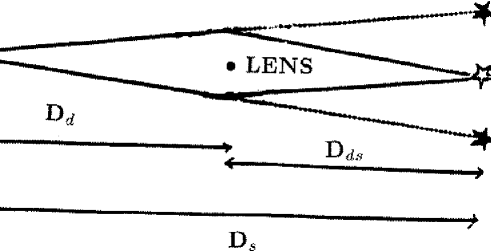
Figure 1: Schematic geometry of the gravitational microlensing. The presence of the lens causes the image of the source to split into two, their combined brightness being always larger than that of the unlensed image. Note that the deflection due to the lens and the separation of the images are greatly exaggerated in this schematic diagram.

With the lensing geometry as described in Figure 1, the Einstein ring radius R_E can be written as

$$R_{E}^{2}={{4GMD}\over{c^{2}}},D={D_{ds}D_{d}\over D_{s}}$$

where M is the the mass of the lensing object, D_d is the the distance to the lensing object, D_ds is the distance from the lens to the source, and D_s is the distance from the observer to the source.

The amplification due to the microlensing depends only on the impact parameter, which can be written as

$$A={{u^{2}+2}\over u(u^{2}+4)^{1/2}}$$

where $u$ is the impact parameter in units of $R_{E}$.

This equation can be easily inverted to derive the impact parameter from a given amplification

$$u=2^{1/2}[A(A^{2}-1)^{-1/2}-1]^{1/2}$$

which can be used to derive the minimum impact parameter $u_{m}$ from an observed light curve.

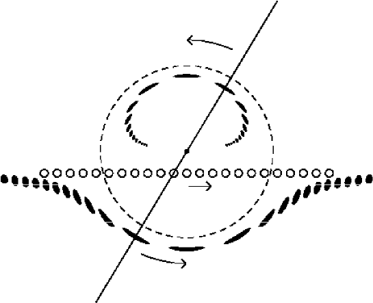
Figure 2: This figure shows how the apparent positions and the sizes of the images change at various stages of the microlensing. In this geometry the position of the lens, indicated by a solid dot, is fixed, and the open circles show the actual positions of the source. The filled circles show the images of the source as the source passes close to the lens in the plane of the sky. The dashed circle is the Einstein ring of the lens. At any instant, the source, the lens and the two images lie on a straight line. (Taken from Paczyński, 1996)

The the time scale of microlensing is the time taken by the source to cross the Einstein ring radius, which is given by

$$t_{0}={R_{E}\over{V_{e}}}$$

where $V_{e}$ is the tangential velocity of the lensing object. The impact parameter at any time during the microlensing event can be expressed as

$$u=[u_{m}^{2}+({t-t_{m}\over t_{0}})^{2}]^{1/2}$$

where $t_{m}$ is the time corresponding to the minimum impact parameter (or the maximum amplification).

From Eq. 1 and 4, the mass of the lens can be expressed as

$$M={[tV_{e}c]^{2}\over{4GD}}$$

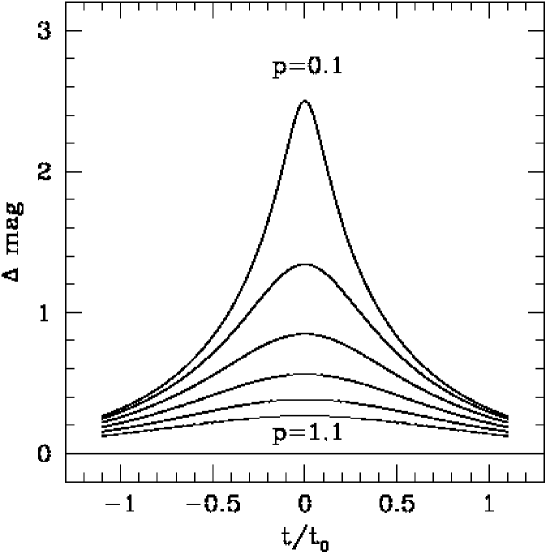
Figure 3: The microlensing light curves as a function of impact parameter.

3.1 Effect of Extended Source

In the case of the microlensing events towards the LMC and the Galactic Bulge, the point-source approximation may not always be valid. This is particularly the case if the LMC events are caused by the LMC stars and the Bulge events are caused by the Bulge stars, in which case the distance between the source and the the lens is not large. Consequently, the Enstin ring radius is smaller, in which case the source size cannot be neglected. (For more details see Sahu, 1994b, Sahu 1997). This is also very important for lensing caused by planetary mass objects since the Einstein ring radius of a planet may not always be much larger than the size of the source. In such a case, different parts of the source will be amplified differently and the net amplification can be expressed as (Eq. 6.81 of Schneider, Ehlers and Falco, 1992)

$${\int d^{2}y\ I(y)\ \mu_{p}(y)\over\int d^{2}y\ I(y)}$$

where I(y) is the surface brightness profile of the source, $\mu_{p}(y)$ is the amplification of a point source at point $y$, and the integration is carried out over the entire surface of the source.

In extended-source approximation, since different parts of the source are amplified differently, the limb darkening effect can be important. This can make the event chromatic and the ratios of the emission/absorption in the star features in the source star can vary during the event (Loeb and Sasselov, 1995). Such effects have indeed been seen in case of MACHO 95-30 (Alcock et al. 1997). The extended source effect can be particularly important in case of planetary events where, in general, the source-size cannot be neglected.

If the source can be approximated as a disk of uniform brightness, then the maximum amplification, when the source and the lens are perfectly aligned, is given by

$$A_{max}=[1+{4R_{E}^{2}\over{r_{0}^{2}}}]^{1\over{2}}$$

where $r_{0}$ is the radius of the source. When the Einstein ring radius is the same as the radius of the source, the maximum possible amplification in such a case is $\sim$2.24.

4 Planets as lenses

4.1 Observational characteristics

The light curve due to a binary lens, unlike the single lens, can be complex and can be very different from the mere superposition of two point lens light curves. In case of a double lens, the lens equation, which is a second order equation for a single lens, becomes two 5th order equations (or one 5th order equation in the complex plane, Witt and Mao, 1995). The most important new feature is the formation of caustics, where the amplification is infinite for a point source, but finite for a finite size source. When the source crosses a caustic, an extra pair of images forms or disappears. A full description of the microlensing due to a double lens is given by Schneider and Weiss (1986).

If the lensing star has a planetary system, the effect of the planet on the microlensing light curve can be treated as that of a binary lens system. The signature of the planet can be seen, in most cases, as sharp extra peaks in the microlensing light curve. Computer codes for analysis of such data have been developed by Mao and Di Stifano (1995) and Dominik (1996).

Figure 4: The figure shows the sizes of the Einstein ring radii R_E at the source plane, for a lensing event towards the Galactic Bulge. R_E for an Earth-mass planet a solar mass star are shown. Also shown are the actual radii of a solar type star and a typical giant star as projected onto the source plane, which are denoted by R(solar) and R(giant) respectively. For a Jupiter-mass planet, R_E is almost always larger than the radius of a giant star, so the effect of Jupiter can always be significant. But for an Earth-mass planet, there is only a small parameter space where the Einstein ring radius is larger than the size of a giant star. If the source is a main-sequence star like our Sun, the Einstein ring radius due to an earth-mass planet is almost always larger than the source size, and hence the amplification can be large.

Figure 5: The same as Fig. 4, but here the sizes of the Einstein ring radii and the sizes of the sources are all as seen projected onto the lens plane.

It was first shown by Mao and Paczyński (1991) that about  10% of the lensing events should show the binary nature of the lens, and this effect is strong even if the companion is a planet. The problem of microlensing by a star with a planetary system towards the Galactic Bulge was further investigated by Gould and Loeb (1992). They noted that, for a solar-like system half way between us and the Galactic Bulge, Jupiter’s orbital radius coincides with the Einstein ring radius of a solar-mass star. Such a case is termed ‘resonant lensing’ which increases the probability of detecting the planetary signal. In $\sim$20% of the cases, there would be a signature with magnification larger than 5%.

The importance of the resonant lensing can be qualitatively understood as follows. In Fig. 2, the impact parameter changes through a large range as the source passes close to the lens. The positions of two images formed by the lensing effect change continuously, but they remain close to the Einstein ring for a large range of impact parameters. So, the effect of the planet can be large if the planet happens to be close to the Einstein ring, which causes a further amplification. This also qualitatively explains why the probability of observing the effect of the planet increases if it is close to the Einstien ring.

In a large number of cases however, the resulting light curve due to a planet plus star system is close to the superposition of two point lens light curves (Fig. 6). This is particularly true when the star-planet distance is much larger than R_E. In such a case, the time scale of the extra peak due to the planet, $t_{p}$, and the time scale of the primary peak due to the star, $t_{s}$, are related through the relation $t_{p}/t_{s}=\sqrt{(m_{p}/M_{s})}$ where $m_{p}$ is the mass of the planet and $M_{s}$ is the mass of the star. Furthermore, if the source size cannot be neglected, the maximum amplification given by Eq. 7 remains valid. Fig. 4 and 5 show the sizes of the Einstein ring radii due to planetary and stellar mass lenses as a function of distance to the lens. The typical sizes of the main-sequence and giant sources are also shown. In such a case, it is clear that the size of the source is almost always smaller than the Einstein ring radius of a Jupiter-mass planet, as a result the amplification due to the planet can be large. The amplification can also be large for an Earth-mass planet if the source is a main sequence star. However, if the source is a giant-type star, then there is only a fixed range of D_d where the amplification due to an Earth size planet can be large.

In general. the situation is different in case of formation of caustics. Fig. 5 shows the effect of the formation of caustics and consequent high amplification and sharp peaks caused by the planets. The planets, in this case, are situated at different orbital radii and the mass of each planet is 10^-3 times that of the primary. The solid curve shows the light curve without the presence of the planets. The dashed and the dotted curves correspond to two representative tracks of the source with the presence of the planets (Wambsganss, 1997).

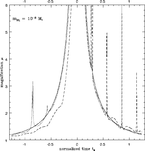
Figure 6: Effect of a few planets situated at different orbital radii on the microlensing light curve. The mass of each planet is 10^-3 times that of the primary. The projected distances of the planets from the primary, in units of R_E, are 0.57, 0.65, 0.74, 0.86, 1.16, 1.34, 1.55 and 1.77. The solid curve shows the light curve without the presence of the planets. The dashed and the dotted curves correspond to two representative tracks of the source with the presence of the planets. This shows how the influence of the planet on the microlensing light curve can be both upward and downward, and illustrates the possible high amplification and sharpness of the extra peaks caused by the planets (taken from Wambsganss, 1997).

The minimum duration of the extra feature due to the planet, to a first approximation, is the time taken by the source to cross the caustic, which can be about 1.5 to 5 hrs. The maximum duration of the spike is roughly the time taken by the planet to cross its own Einstein ring. Using a reasonable set of parameters (the lower mass of the planet is taken as that of the Earth, the higher mass is assumed to be that of Jupiter) this can be a few hours to about 3 days. Any follow-up program must be accordingly adjusted so that the extra feature due to the planet is well sampled.

4.2 Theoretical work

A full description of the theoretical aspects of planets acting as lenses is beyond the scope of this review. To date, there are a few countable number of papers which deals with the theoretical prediction of planetary signals on the light curve, which the reader may refer to (Bolatto and Falco, 1995; Bennett and Rhie, 1996; Wambsganss, 1996; and Peale, 1997).

5 Requirements for a Follow-up Monitoring Program

The first requirement for a follow-up monitoring program is access to the ‘alert’ events. With the alert capability of the survey programs firmly in place, it is now possible to build a follow-up program. At present, the alert events from the MACHO collaboration at a given time is sufficient to carry out a ground based follow up program with small telescopes towards the Galactic Bulge. After OGLE and EROS II experiments have their alert systems in place, the number of on-going alert events at a given time will increase and it may be possible to extend such follow-up networks to larger telescopes, and also perhaps towards the LMC.

The second requirement is the ability to monitor hourly. It should be noted that, assuming that the longer time scale events are mostly due to slower proper motion of the lensing star, the time scale of the planetary signal approximately scales with the time scale of the main event. So the monitoring, in general, can be less frequent for longer time scale events. But typically, as noted before, the time scales of the planetary event can be a few hours to a few days. So the follow-up monitoring program must have the capability to do hourly monitoring so that the extra feature due to the planet is well sampled. For discrimination against any other short term variations, some color information is also useful, since the microlensing is expected to be achromatic, where as most other types of variations are expected to have some chromaticity. Thus it is preferable to have a few observations in two colors.

The third requirement is to have 24-hour coverage in the monitoring program. This calls for telescopes at appropriately spaced longitudes around the globe.

6 A case for an automated telescope in Antarctica

An automated telescope close to the south pole fits the bill perfectly since it not only satisfies all the above requirements, but also has the advantage that it can be operated remotely.

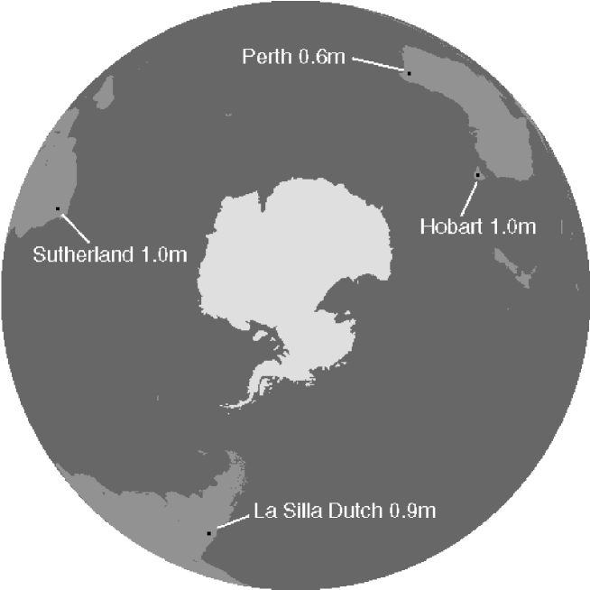
Figure 7: The location of the telescopes used by the PLANET collaboration for follow-up monitoring program of microlensing events (courtesy of PLANET collaboration). A telescope in Antarctica can achieve the same goal of 3 telescopes for 24-hour coverage in the monitoring program.

The PLANET collaboration currently uses 3 or 4 telescopes situated at appropriately spaced longitudes in the southern hemi-sphere to achieve a near-continuous coverage in the monitoring program (Albrow et al. 1995, 1996a,b; 1997). The same can be achieved with a single telescope in Antractica (Fig. 6).

At any given time during the $\sim$3-month period when the galactic bulge is observable, there are typically 8 to 10 on-going microlensing events. This number is likely to increase after the EROS II and OGLE II survey programs have their alert systems fully operational.

With a 1-meter size telescope, about 7 events can be monitored continuously with a sampling interval of 2 to 5 hours required for this project. Taking the typical monitoring duration (which is larger than the microlensing time-scale) to be 1-month, about 20 events can be monitored in a single 3-month period during which the galactic bulge is visible. Since the probability of detection is about 10% if every star has a Jupiter, that should lead to the detection of 2 planetary events in a single season. Even non-detection can provide very strong constraints on the presence of planets around lensing stars. With a bigger telescope, a larger number of events can be monitored, with a correspondingly larger number of expected planetary detections.

Once the number of events towards the LMC and SMC increase, as indeed expected in the near future after the EROS II and OGLE survey programs are fully operational, frequent monitoring of ongoing LMC and SMC microlensing events is a promising possibility. This would make the search strategy sensitive to a very different region in the orbital parameter space, and to a very different group of stars. Both the LMC and the SMC being circum-polar objects, such an extension of the monitoring program will keep the telescope busy for most of the year.

7 Spin-off and other scientific projects

Although the primary goal would be to search for extra-solar planetary systems, numerous other interesting projects can be done with such a telescope, some of which are briefly described below. Most of these projects (1 to 3 below) can be done with the same data and will not need any additional observations.

7.1 Short time-scale and new microlensing events

Since the line of sight towards the galactic bulge passes through the dense concentration of stars in the galactic disk, the optical depth to microlensing in the direction of the bulge is known to be high –   1 x 10^-6. If small mass stars (M $<$ 0.1 M_⊙) contribute significantly to the mass budget of the galaxy, then a sizable fraction of this optical depth would be due to these small mass stars.

The Einsten ring radius of a 0.01 M_⊙ object for a source-lens distance of 1 kpc is about 3 x 10¹² cm (its variation with distance is given by Eq. 1.) Assuming a typical proper motion of about 200 km/s, the time scale for such events would be about 2 days (about 16 hours for m = 0.001 M_⊙ stars). The current microlensing survey programs are insensitive to such short time-scale events and such events would essentially go unnoticed by the survey programs. However, such events can be easily detected by the monitoring program mentioned here with the automated telescope.

There would be typically about 20,000 stars per one 1000 X 1000 pixel CCD image. Thus about 2 $\times$ 10⁶ stars would be observed in about 5 frames. Thus, if 50% of the mass is in form of small mass stars of mass m=0.01 M_⊙, 1 such event would be detected every 2 nights (or about 1 event every 16 hours if m=0.001 M_⊙).

Thus, this program can provide an answer to the contribution of small mass stars to the mass budget of the galaxy. Even non-detection will provide a strong upper limit to their contribution.

In addition, the telescope can be used for detecting new microlensing events. This can perhaps be best done in the near-IR wavelengths where the low extinction allows one to probe deeper into the galactic bulge. The high IR transmissivity near the south pole makes such a project particularly attractive.

7.2 Binary Events

The resolution of sharp caustic crossing in binary events, which may last only a few hours, can be clearly detected from such a monitoring program (Mao & Di Stefano 1995). This can be used to get the binary fraction and characteristics of the lensing objects.

7.3 Extended sources

High-amplification lensing of giants can resolve the structure of the source star. Such an extended source effect can produce chromatic effects that can be quantified through high-quality multi-band photometry near the event peak. Thus the observations can be used to ‘map’ the source star.

7.4 Variable stars

Finally, the resulting data base of frequently-sampled bulge fields, each containing $>$10,000 stars would be clearly useful for the study of variable stars. In addition, the telescope can be used for the purpose of studying some specific variable stars. In particular, the programs which need continuous monitoring for more than 10 hours (e.g. the study of stellar oscillations) can greatly benefit from such a telescope.

- [1] lbrow, M., et al. (PLANET collaboration), 1995, in Proc. IAU Symp. 173, Eds. C.S. Kochanek, J.N. Hewitt, p227
- [2] lbrow, M., et al., 1996a, Proc. 12th IAP Conference, in press (astro-ph/9610128)
- [3] lbrow, M., et al., 1996b, BAAS, 27, 1449
- [4] lbrow, M. et al., 1997, Proc. STScI Symp. on Planets beyond the solar system and the next generation of space missions, Ed. D. Soderblom, ASP Conf. Series.
- [5] lcock, C. et al., 1995, ApJ, 454, L125
- [6] lcock et al., 1997, Preprint (astro-ph/9702199)
- [7] ahcall, J.N., Flynn, C., Gould, A., Kirhakos, S., 1994, ApJ, 435, L51
- [8] ennett D.P, Rhie, S., 1996, ApJ, 472, 660
- [9] olatto, A.D., Falco, E.E., 1994, ApJ, 436, 112
- [10] ominik, M., 1996, Ph.D. Thesis, Univ. Dortmund
- [11] instein, A., 1936, Science, 84, 506
- [12] ould, A., Loeb, A., 1992, ApJ, 396, 104
- [13] riest, K., 1991, ApJ, 366, 412
- [14] ray, D., 1997, Nature, 385, 795
- [15] iraga, M, Paczyński, B., 1994, ApJ, 430, 101
- [16] oeb, A., Sasselov, D., 1995, ApJ, 491, L33
- [17] ao, S., Paczyński, B., 1991, ApJ, 374, L37
- [18] ao, S., Di Stifano, R., 1995, ApJ, 440, 22
- [19] arcy, G.W., Butler, R.P., 1996, ApJ, 464, L153
- [20] ayor, M., Queloz, D.A., 1995, Nature, 378, 355
- [21] aczyński, B., 1986, ApJ, 304, 1
- [22] aczyński, B., 1991, ApJ, 371, L63
- [23] aczyński, B., 1996, Ann. Rev. Astron. Astrophys. 34, 415
- [24] eale, S.J., 1997, Icarus, 127, 269
- [25] ahu, K.C., 1994a, Nature, 370, 275
- [26] ahu, K.C., 1994b, Pub. Astron. Soc. Pac., 106, 942
- [27] ahu, K.C., 1997, “Detecting planets through microlensing”, Proc. STScI Symp. on Planets beyond the solar system and the next generation of space missions, Ed. D. Soderblom, ASP Conf. Series.
- [28] chneider, P., Ehlers, J. & Falco, E.E., 1992, “Gravitational Lensing”, (Springer-Verlag).
- [29] chneider, P., Weiss, A., 1986, Astron. Astrophys. 164, 237
- [30] ambsganss, J., 1997, MNRAS, 284, 475
- [31] itt, H., Mao, S., 1994, ApJ., 430, 505
- [32] olszczan, A., Frail, D.A., 1992, Nature, 355, 145
- [33] u, X-P., 1994, ApJ., 435, 66