Dynamics and Excitation of Radio Galaxy Emission-Line Regions — I. PKS 2356$-$61

Abstract

Results are presented from a programme of detailed longslit spectroscopic observations of the extended emission-line region (EELR) associated with the powerful radio galaxy PKS 2356$-$61. The observations have been used to construct spectroscopic datacubes, which yield detailed information on the spatial variations of emission-line ratios across the EELR, together with its kinematic structure. We present an extensive comparison between the data and results obtained from the MAPPINGS II shock ionization code, and show that the physical properties of the line-emitting gas, including its ionization, excitation, dynamics and overall energy budget, are entirely consistent with a scenario involving auto-ionizing shocks as the dominant ionization mechanism. This has the advantage of accounting for the observed EELR properties by means of a single physical process, thereby requiring less free parameters than the alternative scheme involving photoionization by radiation from the active nucleus. Finally, possible mechanisms of shock formation are considered in the context of the dynamics and origin of the gas, specifically scenarios involving infall or accretion of gas during an interaction between the host radio galaxy and a companion galaxy.

KOEKEMOER & BICKNELL RADIO GALAXY EMISSION-LINE REGIONS: PKS 2356$-$61

Space Telescope Science Institute, 3700 San Martin Drive, Baltimore, MD 21210, USA; koekemoe@stsci.edu

ANU Astrophysical Theory Centre, Australian National University, Canberra, ACT 0200, Australia (The ANUATC is operated jointly by the Mount Stromlo and Siding Spring Observatories and the School of Mathematical Sciences of the Australian National University); gvb@maths.anu.edu.au

galaxies: active — galaxies: individual (PKS 2356$-$61) — galaxies: ISM — galaxies: kinematics and dynamics — radio continuum: galaxies — shock waves

1997 June 26 1997 November 7

To appear in The Astrophysical Journal

1 Introduction

Powerful radio galaxies are often observed to contain systems of ionized gas, extended up to scales of several tens of kpc from the nucleus. Detailed studies of these extended emission-line regions (EELRs) have revealed a wide range of morphological and kinematic properties (e.g., Baum & Heckman 1989a, 1989b; Tadhunter, Fosbury & Quinn 1989; McCarthy, Spinrad, & van Breugel 1995): in some objects the EELR is coincident with the radio lobes, while in the majority of cases the line-emitting gas is extended at modest angles away from the radio axis and does not display a direct spatial association with the radio emission. The EELR kinematics (Tadhunter et al. 1989; Heckman et al. 1989; Baum et al. 1992) can be generally classified into “rotators” and “non-rotators”, the latter being further subdivided into “calm” and “violent”. The rotator EELRs typically exhibit circular velocity fields approximately consistent with the massive halos inferred for radio ellipticals, while the non-rotators display less well-ordered kinematics and little or no evidence of settled dynamics.

Explanations for the origin of the gas include mergers or interactions involving gas-rich galaxies; large differences between the gaseous and stellar kinematics (Phillips et al. 1986; Tadhunter et al. 1989; Bettoni et al. 1990) suggest external infall of gaseous material on recent timescales compared to the age of the elliptical (Habe & Ikeuchi 1985, 1988; Varnas et al. 1987). Detailed kinematic studies of EELRs often reveal a correspondence between the radio axis and the gas “rotation” axes (e.g., Simkin 1977; Heckman et al. 1985; Tadhunter et al. 1989), suggesting a direct connection between gas infall and nuclear activity. It has also been suggested that the gas has condensed out of a hot intergalactic medium (Fabian et al. 1981; Canizares et al. 1987); however, the angular momentum of gas in radio galaxies tends to be higher than that of typical cooling flow EELRs. Furthermore, the importance of mergers in fuelling galaxy activity is suggested by the typical morphological disruption of host galaxies (Hutchings 1987; Smith & Heckman 1989) as well as apparent environmental differences between radio-loud and normal ellipticals (Lilly & Longair 1984; Spinrad & Djorgovski 1984).

Thus, a principal question in the study of the formation and evolution of radio galaxies concerns the detailed physical properties of the EELRs. In particular, models of the EELR ionization and dynamics are of importance in understanding their origin, as well as their rôle as a source of fuel for the active nucleus, related to the more general question of the triggering mechanism for active galaxies.

Excitation of radio galaxy EELRs has generally been considered in the context of “unified schemes” of radio galaxies and quasars (e.g., Barthel 1989), involving photoionization of the gas by radiation from the active nucleus. This is analogous to the scenario inferred on kpc scales for EELRs in Seyfert galaxies, where nuclear photoionization is supported by “ionization cones” in line-ratio maps in a number of objects, and by the presence of polarized broad emission lines (e.g., Antonucci & Miller 1985; Mulchaey, Wilson, & Tsvetanov 1996). While evidence for orientation-based unification of radio galaxies and quasars has been inferred from a range of observational studies, including radio galaxy morphology and beaming studies, X-ray properties, and host galaxy populations (e.g., Antonucci 1993 and references therein; see also Gopal-Krishna, Kulkarni, & Wiita 1996), it is less clear that all the detailed properties of the line-emitting gas in all radio galaxies can be explained in terms of nuclear photoionization. Firstly, radio galaxy EELRs are extended on much larger scales than those in Seyfert galaxies, typically by at least an order of magnitude, and do not display clear ionization cones. Furthermore, relationships between EELR luminosity and core power or total radio power typically display a scatter of $1-2$ orders of magnitude (e.g., Baum & Heckman 1989b), which may be due in part to different ionization mechanisms dominating in different objects that have otherwise similar core properties. Another interesting effect is that the global kinematic properties of EELRs have been shown to correlate with their overall excitation state; this is not a directly expected consequence of unified schemes, and suggests the importance of local ionization in some classes of objects (Baum et al. 1990, 1992).

Moreover, detailed studies of individual radio galaxies have shown that the EELR properties cannot always be readily accounted for in terms of nuclear photoionization. Specifically, the extended material in a number of objects display emission-line fluxes and excitation states that are inconsistent with the nuclear ionization properties required to photoionize the material closer to the AGN (e.g., Danziger et al. 1984; van Breugel et al. 1986; Tadhunter et al. 1988; Meisenheimer & Hippelein 1992). In such objects, the importance of local ionizing mechanisms, such as shocks, has been postulated in order to explain the large-scale properties of the extended gas. Thus, while orientation effects are clearly likely to affect some observational properties of radio galaxies and quasars, we point out that the ionization and excitation properties of the EELRs may be dominated to varying degrees in individual objects by local ionization mechanisms, related for example to shocks.

In this paper we address in detail the feasibility of “auto-ionizing shocks” as a viable ionization mechanism for the extended gas. One possible origin for shocks is collisions between streams of gas during a galaxy merger. This scenario is motivated by the “tidal” EELR morphology often observed in radio sources, where the gas is neither conical nor directly associated with the radio plasma. In objects where the radio plasma coincides with the EELR (e.g., Prieto et al. 1993; Tadhunter et al. 1994) it is possible that associated bowshocks may play a direct role in ionizing the gas. For example, the auto-ionizing shock model has been applied successfully to observations of emission-line gas in Centaurus A (Sutherland, Bicknell & Dopita 1993). The physical appeal of auto-ionizing shocks is that the gas energetics, excitation and kinematics are accounted for in a single, physically self-consistent model, requiring less free parameters than photoionization by a hidden AGN.

2 Observational Programme

2.1 Target Object

In order to obtain as complete a description as possible of the physical properties of the gas, a combination of kinematic and excitation information is required across its entire extent. We describe the results from a program of low- and high-dispersion longslit spectroscopy of the radio galaxy PKS 2356$-$61, sampling the EELR completely through the use of multiple slit positions.

The radio galaxy PKS 2356$-$61 is one of the strongest southern FR II sources, with a total radio power $P_{\rm 1.4\,GHz}\sim 10^{25.8}\,$W Hz^-1, and was discovered during the “Mills Cross” radio survey of the southern sky by Mills et al. (1961). Its double-lobed morphology has been apparent since the first radio synthesis observations were obtained (Ekers 1969). The optical counterpart was identified by Westerlund & Smith (1966) to be a type E3 or D elliptical of $V$ magnitude 16, in a sparsely populated field (containing 10 other galaxies within a region $\sim 21\arcmin$ in size, i.e., $\sim 2.3\,$Mpc for ($H_{0}=75{\rm\,km\,s^{-1}}\,$Mpc^-1, $q_{0}=0$, which we use throughout this paper). The first redshift determination was by Whiteoak (1972), who measured a value of $z=0.0959$ based on optical emission-lines. A nuclear spectrum obtained by Danziger & Goss (1983) shows strong, high-excitation narrow-line emission, with a high [OIII]$\lambda$5007/H$\beta$ ratio ($\gtrsim 10$) and the presence of significant [NeV]$\lambda$3426. This is also evident in the fluxes published by Robinson et al. (1987) for the nuclear region and two off-nuclear regions (7 E and 4 W). These and other optical properties are summarized in Table 2.1.

lrl 0pt General properties of PKS 2356$-$61. & Notes R.A. (B1950) & $23^{\rm h}\;56^{\rm m}\;29\fs 37\;\pm\,0\fs 02$ 1,2 Dec. (B1950) $-61\arcdeg\;11\arcmin\;40\farcs 6\;\pm\,0\farcs 5\!\phn$ 1,2 $z_{\rm abs}$ 0.0963 $\pm\,0.0001$ 3 $z_{\rm em}$ 0.0959 $\pm\,0.0001$ 3,4 $z_{\rm abs+em}$ 0.0958 $\pm\,0.0003$ 5 Distance $D_{L}$ $z_{\rm abs+em}$ (Mpc)^† 383           Scale (kpc/arcsec)^† 1.86           Galaxy type D/E3          1,2,6 $V$ mag. 16           1 $B$ mag. 17           6,7 Continuum extent $6\arcsec\times 4\arcsec$        1 Continuum P.A. $6\arcdeg$           1 EELR extent $14\arcsec\times 8\arcsec$        8 $F_{\rm[OIII]\lambda 5007}/F_{\rm H\beta}$ 13.2           9 $F_{\rm H\beta}$(erg/s/cm²) $3.94\times 10^{-15}$     9 $\Delta V_{\rm tot}$ (km s^-1) 180           8 $\Delta V_{\rm max}$ (km s^-1) 90           8 $P_{\rm 1.4\,GHz}$ (W Hz^-1) $6.3\times 10^{25}$     10 1: Westerlund & Smith 1966; 2: Ekers 1970; 3: Tritton 1972; 4: Whiteoak 1972; 5: Danziger & Goss 1983; 6: Sutton 1968; 7: Tadhunter et al. 1989; 8: Danziger & Focardi 1988; 9: Robinson et al. 1987; 10: Wright & Otrupcek 1990.
^† We use $H_{0}=75{\rm\,km\,s^{-1}}\,$Mpc^-1, $q_{0}=0$.

The only previously published emission-line image is in H$\alpha$ (Danziger & Focardi 1988), showing a bright, elongated emission-line region centred on the galaxy nucleus, with an arc or shell-like feature on its eastern side. A very faint tail extends from the east to the south; a high-dispersion longslit spectrum of one of the blobs in this tail (Tadhunter et al. 1989) shows a relatively small velocity gradient ($\lesssim 200{\rm\,km\,s^{-1}}$).

2.2 Observations and Data Reduction

The observations were obtained during dark time on the nights of 1 and 2 August, 1992, using the RGO Spectrograph mounted at the f/8 Cassegrain focus of the Anglo-Australian Telescope (AAT). The detector used was the Tektronix #2 CCD, which consists of $1024\times 1024$ 24 pixels, each corresponding to 077 on the sky. Details of the observations are presented in Table 2.2. Conditions were sufficiently photometric that reliable absolute photometry was obtained, and the seeing ranged between 12 and 15. A detailed account of the observations and reduction procedures is presented in Koekemoer (1996).

lcc 0pt Spectrophotometric Observations of PKS 2356$-$61. & 1 August 1992 2 August 1992 Grating & 270R 1200V
Wavelength/pixel 3.39 Å 0.58 Å
Spectral range 3996$\,\rightarrow\,$7465 Å 5305$\,\rightarrow\,$5895 Å
Emission lines [OII]$\lambda$3727$\rightarrow$[SII]$\lambda$6731 H$\beta$, [OIII]$\lambda$5007
Calibration arcs He/Ne/Ar Cu/Ar
The data obtained each night consisted of exposures in 14 parallel, adjacent slit positions at a position angle of 0. The slit width was 1 and the slit positions were offset in R.A. in increments of 1; the spatial coverage extended from $5\arcsec\,$W$\,\rightarrow\,8\arcsec\,$E of the nucleus. The exposure time at each slit position totaled 1200 sec.

Longslit exposures were obtained at parallel positions across the entire extent of the EELR, thereby producing two spectral datacubes (at high- and low-dispersion) in Right Ascension, Declination and wavelength. New slit positions were acquired by offsetting the telescope in increments of 1. This is most reliably achieved through the use of “Star-to-Probe” guiding: the guiding assembly is moved by a specified amount, and the telescope moves automatically in order to re-position the guide star on a standard location. By re-acquisition of the galaxy nucleus and nearby stars throughout the night, it was verified that positioning errors were $\lesssim 0\farcs 15$.

Longslit observations are susceptible to problems due to atmospheric effects. Seeing fluctuations can cause changes in the contribution from regions immediately outside the slit, while low-dispersion data can suffer from differential refraction, resulting in varying contributions from regions outside the slit as a function of wavelength. However, all the data were obtained at zenith distances $\lesssim 30-40\arcdeg$, thus differential refraction effects are $\lesssim 0\farcs 2$ along the wavelength regime covered. The impact of these effects was further minimized by employing a slit width of 1, comparable to the seeing disk size, and by spatially smoothing the final dataset using 3$\times$3-pixel averaging.

Smooth-spectrum stars and photometric standards (Baldwin & Stone 1984) were observed to correct for atmospheric absorption lines and the detector/grating spectral response. Routines in the IRAF “onedspec” package were used to apply these corrections to the data. Frames were de-biased using the corresponding overscan regions, and no two-dimensional bias structure was present on the detector. Pixel-to-pixel flat-fields were obtained from exposures of the internal tungsten lamp. The frames were corrected for optical vignetting along the slit using twilight exposures obtained with the same slit width. The spectra were corrected for atmospheric extinction using standard extinction curves for Siding Spring Observatory (available within IRAF).

Internal arc exposures were obtained at regular intervals throughout each night, in order to correct for instrumental shifts. A two-dimensional wavelength transformation for each arc frame, subsequently applied to the data, was obtained by fitting arc lines at multiple positions along the slit, using routines in the IRAF “twodspec” package. The resulting residuals in wavelength were less than 0.1 pixels across the regions of interest. After wavelength calibration, the night-sky spectrum for each frame, obtained from empty regions along the slit, was subtracted from the data.

3 Results

3.1 Morphology

We used the low-dispersion datacube to investigate the spatial distribution of the stellar continuum and emission-line gas in PKS 2356$-$61. The datacube was smoothed in R.A. and Dec. using a “boxcar” filter ($3\times 3$ pixels), in order to minimise effects due to possible changes in seeing throughout the night. A continuum image, shown in Figure 1$a$, was produced by summing all channels with observed wavelengths in the range $5591-6685$Å (i.e., rest wavelengths of $5100-6100$Å, corresponding approximately to $V$-band), taking care to avoid the 5577Å night sky line as well as [OIII]$\lambda$5007 and other strong emission lines. We fitted elliptical isophotes to the host galaxy in this image using the IRAF/STSDAS package “ellipse” (Jedrzejewski 1987), and compared the results with ellipses fitted on a broad-band CCD image of the object. In neither case did we find any significant residual continuum features co-incident with the emission-line region; instead, the stellar continuum follows a well-behaved elliptical light distribution. Furthermore, the radial distribution of surface brightness, ellipticity and position angle as derived from the spectroscopic datacube showed excellent agreement with those obtained from the CCD image, confirming that the datacube is capable of yielding spectrophotometric results as reliable as those obtained using conventional imaging photometric techniques.

Some faint, extended continuum emission appears to be associated with the objects toward the north of the source; this is also evident on the broad-band CCD image. Spectroscopically, this structure is associated with H$\alpha$ emission at very similar systemic velocities to the gas in the central source; it is therefore likely that this material is dynamically associated with the central galaxy. The brighter objects, however, are foreground stars, as confirmed by examination of their summed low-dispersion spectra.

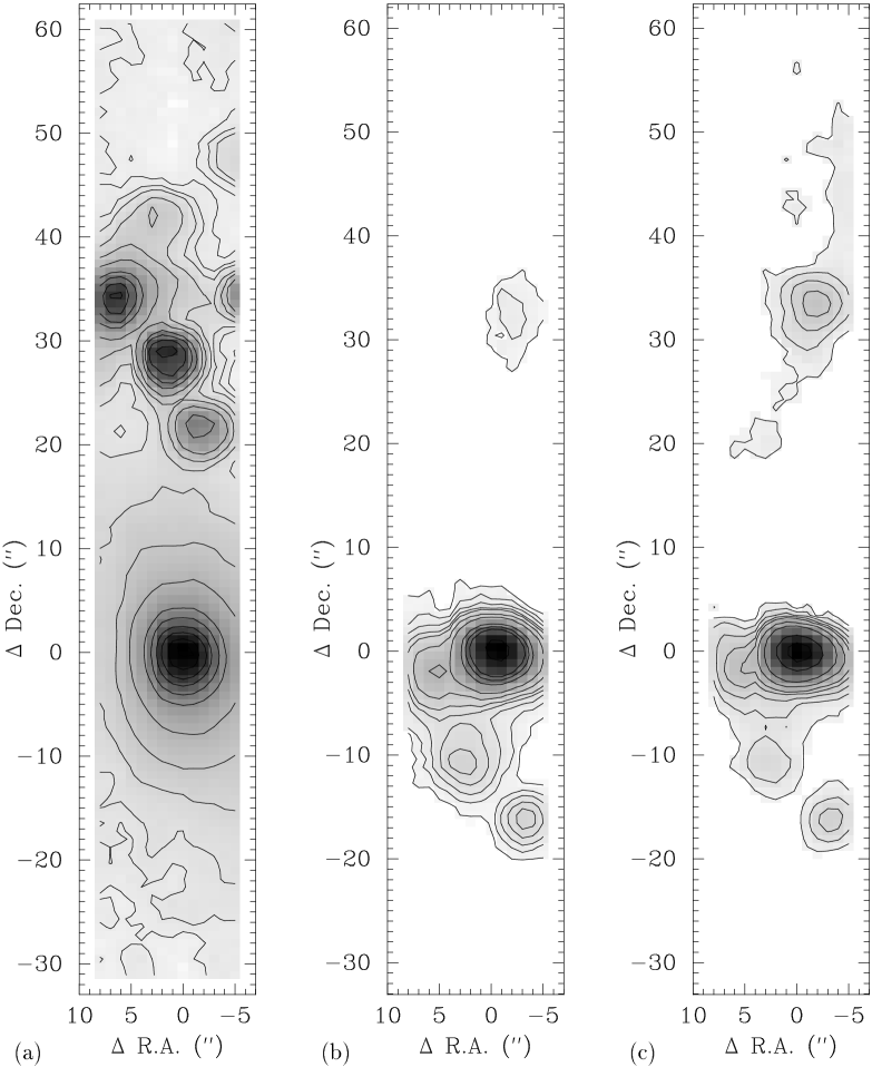
Figure 1: Images of PKS 2356$-$61 derived from the low-dispersion spectral datacube. Positions are given in offsets of R.A. and Dec. relative to the nucleus; North is to the top and East is to the left in all images. $(a)$ “$V$-band” continuum image; $(b)$ [OIII]$\lambda$5007 image; $(c)$ H$\alpha$ image. In all images the slit is oriented north-south and pixel sizes are $1\arcsec\times 0\farcs 77$ (corresponding to a slit width of 1, with a spatial scale along the slit of 077/pixel). Pixels along the slit have not been rebinned into 1 increments, in order to avoid the introduction of artifacts due to non-uniform resampling of flux. Instead, the aspect ratio of pixels is plotted in such as way that the spatial scale in arcseconds is the same along each axis.

“Narrow-band” images of the emission-line gas in [OIII]$\lambda$5007 and H$\alpha$ are presented in Figures 1$b$,$c$. These were obtained by parameterizing the line profiles in terms of Gaussian components. All pixels containing detectable line emission were fitted using the “specfit” routine within IRAF, yielding values and error estimates for the fluxes, velocities and widths of the lines [OIII]$\lambda$5007, H$\beta$, H$\alpha$, [NII]$\lambda\lambda$6548,6583 and [SII]$\lambda\lambda$6716,6731. The spectral resolution is $\sim 4$Å, sufficiently high to separate the H$\alpha$ and [NII] profiles but also low enough that each line profile can be adequately described by a single Gaussian. The resulting images in Figures 1$b$,$c$ represent all pixels with flux values greater than the corresponding formal 3-$\sigma$ limits obtained from the fits.

The emission-line region associated with the host galaxy may be described generally in terms of two components, a bright elongated central region and a fainter tail extending up to $\sim 15-20\arcsec$ from the nucleus. The tail itself consists of three distinct clouds which we designate A, B and C, in order of increasing distance from the central region. No association with the radio axis (at PA $\sim 135$) is evident, either in the central region or in the tail. However, it is interesting to note that the major axis of the central region is approximately perpendicular to the orientation of the host galaxy optical continuum distribution.

A large H$\alpha$-emitting region is evident to the north of the host galaxy, displaying relatively little [OIII] $\lambda$5007 emission. This region corresponds to the faint, diffuse emission apparent in the continuum image. A faint extension can be seen on either side of its central component; the total projected length of these extensions is $\sim 55\,$kpc. The systemic velocity of this object is within $\sim 200{\rm\,km\,s^{-1}}$ of that of the central galaxy, and this is considerably smaller than expected if two cluster objects were randomly superimposed (in which case the velocity difference should be comparable to the projected cluster velocity dispersion, i.e., $\gtrsim 1000{\rm\,km\,s^{-1}}$). Thus, it is possible that the H$\alpha$ object corresponds to a gas-rich galaxy that is interacting with the host galaxy of PKS 2356$-$61, in which case its extended morphology may be accounted for by tidal disruption.

3.2 Kinematics

The high-dispersion spectral datacube has a velocity FWHM resolution $\sim 70{\rm\,km\,s^{-1}}$, the spectral sampling being 0.8Å. The observations were taken at the same slit positions and offsets as those used for the low-dispersion datacube, but the data were obtained on a different night, so that seeing effects could potentially introduce differences in the flux distribution compared to the low-dispersion datacube. In order to minimize such effects, the dataset discussed here has been smoothed in the same way as the low-dispersion dataset, by using a “boxcar” filter of $3\times 3$ pixels.

In Figure 2 we present several different views of the continuum-subtracted [OIII]$\lambda$5007 datacube. These images were created with the AVS package. The orientations in all panels are such that redshift increases towards the right. The top left panel (Fig. 2$a$) shows the flux distribution of the gas as viewed on the sky, with north toward the top and east to the left. The cube is then presented at a number of different viewing angles; for example, Figure 2$d$ shows the equivalent of a longslit spectrum covering the whole emission-line region — in this image, north is at the top and south is at the bottom (i.e., the slit direction runs vertically along the page).

Figure 3: High-dispersion [OIII]$\lambda$5007 velocity structure of the emission-line gas in PKS 2356$-$61. Each spectrum represents the sum of a region $\sim 3-4\arcsec$ across, i.e., larger than the scale used for smoothing the datacube, thus adjacent spectra are independent of one another. All velocities are relative to the systemic velocity (mean emission-line redshift of the entire system), which is indicated by the vertical axis. The orientation of this image is the same as in Figure 1; North is toward the top and East is to the left.

A more quantitative representation of the velocity structure is shown in Figure 3; a comparison of these data with Figure 2 reveals that the three clouds comprising the tail are spatially and kinematically distinct, having different central velocities as well as different internal velocity fields. However, the velocity widths of individual components in these clouds are almost all the same, ranging from 120 to 150${\rm\,km\,s^{-1}}$. Here we describe the general characteristics of the tail clouds.

Cloud C has a higher redshift than any of the other gas components in the EELR. It contains only one velocity component, with an almost constant velocity width. The velocity centroids also show little or no systematic change across the entire extent of this cloud.

Cloud B is at a lower redshift and is comprised of two kinematically distinct components, B1 and B2, at lower and higher redshifts respectively. These components both have a very similar velocity width to the gas in C, and the width also appears to remain constant across their entire extent. Furthermore, they overlap almost entirely on the sky and their surface brightnesses are very similar. Component B1 shows no systematic change in velocity centroid but B2 displays a smooth velocity gradient across its entire extent, being more redshifted in the direction of C. A faint connection may be seen between B2 and C, but this is possibly a result of the smoothing since the unsmoothed dataset contains a set of pixels between the two clouds where there is no detectable [OIII]$\lambda$5007 emission. The velocity gradient is not a result of the smoothing since it extends over many smoothing scales.

Cloud A contains a bright component with a width similar to that of cloud C but it also contains a fainter, broader, blue-shifted component. The bright component shows no systematic change in its velocity centroid, which is intermediate between those of the two components in B. Its velocity centroid is also very close to the value of the systemic velocity. The faint broad blue extension in A is characteristic of a “blue wing” although given its low S/N, it could also be a single separate component, as is the case for B. The faint component is considerably broader, having approximately the same width as the total difference between the two components in B. A significant spatial overlap is apparent between clouds A and B, even in the unsmoothed datacube.

The central component is kinematically distinct from the clouds in the tail. It is dominated by a broad component, with FWHM values $\sim 300-400{\rm\,km\,s^{-1}}$, and also has a much higher surface brightness than any of the tail regions. This region also contains asymmetric extensions to the main component, possibly indicating narrow components similar to those found in the tail clouds; these could also be due to the presence of blue and red wings.

3.3 Emission-Line Ratios

We next consider the physical conditions and excitation state of the gas, using the spatial variation of a number of emission-line ratios across the EELR as derived from the low-dispersion datacube. In this sub-section we present several emission-line ratio maps, followed by composite spectra for a number of sub-regions within the EELR.

3.3.1 Line-Ratio Images

In Figure 4 we present images of the spatial variation of the line ratios [OIII]$\lambda$5007/H$\beta$, [NII]$\lambda$6583/H$\alpha$, [SII]$\lambda\lambda$6716+6731/H$\alpha$, [SII]$\lambda\lambda$6716/6731, and H$\alpha$/H$\beta$.

An important consideration in quantifying the Balmer line fluxes is the degree of Balmer absorption present in the underlying stellar continuum. This has been addressed in the literature using a variety of techniques (e.g., Koski & Osterbrock 1976; Filippenko & Sargent 1988; Storchi-Bergmann et al. 1992), generally involving an independent determination of the stellar continuum. However, in PKS 2356$-$61 there are no strong emission-line free regions of continuum, and the continuum is also too faint to allow an unambiguous determination of the intrinsic degree of absorption, for example by using synthetic stellar spectra.

Instead, the significance of stellar absorption may be determined through a comparison of the variation of the ratio H$\alpha$/H$\beta$ and the stellar continuum. It can be seen in Figure 4$e$ that a strong peak in this ratio is present at a location immediately to the east of the nucleus, increasing by almost a factor of 2 to values in the range $5-6$. Since the stellar continuum is relatively weak, a drastic change in stellar population would be required to account for this effect by Balmer line absorption; however, no such change is observed in the host galaxy continuum spectra. Thus we infer that the variations in H$\alpha$/H$\beta$ across the central EELR are indicative of intrinsic variations in the amount of extinction, and not the result of underlying absorption. In the tail, however, there is a possibility of significant underlying absorption in the continuum, which we discuss further when presenting the one-dimensional low-dispersion summed spectra.

Examination of the line-ratio images reveals the presence of a “band” of excitation across the nucleus, extending towards the south-west and north-east. This feature is particularly apparent on the images of [OIII]$\lambda$5007/H$\beta$ and [NII]$\lambda$6583/H$\alpha$, displaying typical line ratio values of [OIII]$\lambda$5007/H$\beta$ $\sim 10$, [NII]$\lambda$6583/H$\alpha$ $\gtrsim 1$ and [SII]$\lambda\lambda$6716+6731/H$\alpha$ $\sim 0.9$. Upon moving away from the nucleus, two clear trends in excitation are evident: (1) towards the south-east and north-west, i.e., in a direction perpendicular to the band, the [OIII]$\lambda$5007/H$\beta$ ratio increases to around $15-20$ while [NII]$\lambda$6583/H$\alpha$ decreases to $\sim 0.5-0.6$, and [SII]$\lambda\lambda$6716+6731/H$\alpha$ also decreases to $\sim 0.5$; (2) along the band, towards the south-west and north-east, the behaviour is somewhat inverted, with [OIII]$\lambda$5007/H$\beta$ remaining at a value $\sim 10$ and [NII]$\lambda$6583/H$\alpha$ increasing to values $\gtrsim 1.2$. The band also coincides with the region of high reddening inferred from the H$\alpha$/H$\beta$ ratio, suggesting that this region may correspond to a ring or disk of dust-rich material. The one-dimensional composite spectra discussed in the following sub-section allow a more detailed investigation of the physical properties of various regions in the EELR.

3.3.2 Composite Spectra

Low-dispersion composite spectra are presented in Figure 5 for the entire central emission-line region, the nucleus ($3\arcsec\times 3\arcsec$), and the summed emission from the three tail regions A, B and C. The wavelength scales of the spectra have been corrected to rest wavelength, using the mean redshift of the brightest emission lines.

Figure 5: Low-dispersion spectra (rest wavelength) for: $(a)$ the central region, $(b)$ the nuclear region ($3\arcsec\times 3\arcsec$), and $(c)$ the entire tail region. These spectra were produced by summing all the individual spectra corresponding to pixels that have a detectable [OIII] flux in the emission-line image, and thus represent high S/N integrated spectra for each region.

In Figure 6, we present the summed spectra for the H$\alpha$ object to the north of PKS 2356$-$61. Its spectrum is typical of a star-forming region, with a very young stellar population and strong Balmer and [OII]$\lambda$3727 emission, with very little [OIII]$\lambda$5007. It is interesting to note that the two extensions both show some emission-line features, although their stellar continua are very different. In particular, the southern extension has a spectrum very similar to the nucleus of the object, while the northern extension has a much larger Balmer line equivalent width, displaying very little continuum emission. This may indicate that the northern extension consists almost exclusively of star-forming regions, while the stronger continuum in the nucleus and southern extension reveals the additional presence of somewhat older stars; a more definitive interpretation is precluded by the relatively low S/N.

Figure 6: Low-dispersion spectra (rest wavelength) for the faint H$\alpha$ object to the north of PKS 2356$-$61. These spectra were produced in the same way as those presented in Figure 5, by summing all the individual spectra corresponding to pixels with a detectable H$\alpha$ flux. The top panel (a) shows the total summed spectrum for all pixels covering the entire H$\alpha$ object, including the northern and southern extensions and its central region. The second and third panels (b) and (c) display the spectra for the southern and northern extensions, and are shown here in order to afford a comparison between the two extensions and the total spectrum, the differences possibly being a result of different stellar populations in each region.

lrlrlrlrlrl 0pt Line fluxes and errors for the low-dispersion spectra of PKS 2356$-$61. Emission & Centre Tail (Tot.) Tail (A) Tail (B) Tail (C)
line Flux 1-$\sigma$ Flux 1-$\sigma$ Flux 1-$\sigma$ Flux 1-$\sigma$ Flux 1-$\sigma$ [OII]$\lambda$3727 226.0 3.4 10.9 0.6 5.14 0.87 3.26 0.82 1.03 0.65 [NeIII]$\lambda$3869 54.3 2.1 4.53 0.51 2.20 0.64 H$\gamma$ 35.8 1.7 2.45 0.45 0.47 0.36 [OIII]$\lambda$4363 20.7 1.6 1.88 0.40 HeII$\lambda$4686 19.4 1.2 1.84 0.33 H$\beta$ 53.0 1.2 2.35 0.43 1.33 0.26 0.60 0.29 0.47 0.21 [OIII]$\lambda$5007 662.0 1.8 38.3 0.7 19.4 0.5 11.0 0.4 4.48 0.28 [NI]$\lambda$5200 9.95 1.06 0.67 0.41 0.35 0.23 [OI]$\lambda$6300 32.7 1.2 0.60 0.35 0.33 0.21 H$\alpha$ 229.0 1.4 10.1 0.6 4.98 0.26 2.54 0.28 1.68 0.23 [NII]$\lambda$6583 203.0 3.7 7.12 0.57 3.02 0.27 2.18 0.30 1.11 0.22 [SII]$\lambda$6716 95.0 2.2 1.27 0.63 0.93 0.42 [SII]$\lambda$6731 70.3 1.7 1.67 0.58 0.77 0.37 All values are in units of $1\times 10^{-16}\,$erg s${}^{-1}\,$cm^-2.

lrrrrr 0pt De-reddened line ratios for PKS 2356$-$61. Line Ratio Centre Tail (Tot.) Tail (A) Tail (B) Tail (C) $C$ 1.169   1.189   0.761   1.125   0.647   3pt HeII$\lambda$4686/H$\beta$ 0.39 ${}_{0.36}^{0.42}$ 0.84 ${}_{0.62}^{1.13}$ [OIII]$\lambda$5007/H$\beta$ 11.9 ${}_{11.6}^{12.2}$ 16  ${}_{14}^{19}$ 14  ${}_{12}^{17}$ 18 ${}_{12}^{30}$ 9.5 ${}_{~{}7.1}^{13.3}$ [OIII]$\lambda\lambda$5007+4959/4363 34.5 ${}_{31.9}^{37.5}$ 22  ${}_{19}^{27}$ [OIII]$\lambda$5007/[OI]$\lambda$6300 27.4 ${}_{26.4}^{28.6}$ 87 ${}_{~{}57}^{179}$ 72 ${}_{~{}47}^{146}$ [OIII]$\lambda$5007/[OII]$\lambda$3727 1.90 ${}_{1.87}^{1.94}$ 2.3  ${}_{2.2}^{2.4}$ 2.8  ${}_{2.5}^{3.3}$ 2.2 ${}_{1.8}^{2.9}$ 3.4 ${}_{2.4}^{5.9}$ [OIII]$\lambda$5007/[NII]$\lambda$6583 4.69 ${}_{4.59}^{4.79}$ 7.9  ${}_{7.3}^{8.5}$ 8.2  ${}_{7.5}^{8.9}$ 7.2 ${}_{6.3}^{8.3}$ 4.9 ${}_{4.3}^{5.7}$ [OIII]$\lambda$5007/H$\alpha$ 4.15 ${}_{4.12}^{4.19}$ 5.6  ${}_{5.3}^{6.0}$ 4.9  ${}_{4.7}^{5.2}$ 6.2 ${}_{5.5}^{6.9}$ 3.3 ${}_{3.0}^{3.6}$ [OI]$\lambda$6300/H$\alpha$ 0.15 ${}_{0.14}^{0.16}$ 0.06 ${}_{0.03}^{0.10}$ 0.07 ${}_{0.03}^{0.11}$ [SII]$\lambda\lambda$6716+6731/H$\alpha$ 0.70 ${}_{0.68}^{0.72}$ 0.28 ${}_{0.21}^{0.37}$ 0.34 ${}_{0.20}^{0.48}$ [NII]$\lambda$6583/H$\alpha$ 0.89 ${}_{0.87}^{0.91}$ 0.71 ${}_{0.63}^{0.79}$ 0.60 ${}_{0.54}^{0.67}$ 0.86 ${}_{0.70}^{1.05}$ 0.66 ${}_{0.56}^{0.78}$ [SII]$\lambda\lambda$6716/6731 1.35 ${}_{1.29}^{1.42}$ 0.76 ${}_{0.36}^{1.46}$ 1.2  ${}_{0.6}^{2.7}$ The ratio upper and lower limits are derived from the 1-$\sigma$ flux errors.

Line fluxes were measured using the IRAF routine “specfit”; since these spectra are of low dispersion, each profile can be adequately described by a single Gaussian component. In clouds B and C, the [SII] lines were not fitted due to the noise contribution from skylines at 7300Å. Table 3.3.2 lists the measured fluxes and 1-$\sigma$ rms errors for all the lines fitted. The errors are the formal 1-$\sigma$ errors obtained from the fits, but they do not represent other effects such as sky background subtraction uncertainties. Thus their primary use is simply to give an indication of the relative accuracy of the various measured fluxes, particularly relevant to the fainter regions.

In Table 3.3.2 we present a number of physically important line ratios, corrected for reddening effects using several standard assumptions. The intrinsic ratio $I_{\lambda_{1}}/I_{\lambda_{2}}$ of the intensities of two lines at wavelengths $\lambda_{1}$,$\lambda_{2}$, given an observed ratio $I_{\lambda_{1,0}}/I_{\lambda_{2,0}}$ and an extinction function $f(\lambda)$ (e.g., Savage & Mathis 1979), is calculated following Osterbrock (1989):

$${I_{\lambda_{1}}\over I_{\lambda_{2}}}={I_{\lambda_{1,0}}\over I_{\lambda_{2,0}}}\,e^{C[f(\lambda_{1})-f(\lambda_{2})]}$$

where the optical depth at $\lambda$ is $\tau_{\lambda}=C\,f(\lambda)$, parameterized by the coefficient of extinction $C$. Extinction due to our galaxy is assumed negligible as a result of the relatively high galactic latitude of the source ($-55\arcdeg\,$S), thus all reddening is considered to be internal to the source. Case B recombination is assumed, with the canonical H$\alpha$/H$\beta$ ratio of 2.87. Although some authors claim evidence of a slightly higher intrinsic ratio of $\sim 3.0-3.1$ when a hard ionizing spectrum is assumed (Halpern & Steiner 1983; Ferland & Osterbrock 1985; Tsvetanov & Yancoulova 1989), we find that this difference has a negligible effect on the present results. Underlying Balmer-line absorption is also taken to be negligible, as we discussed previously based on the H$\alpha$/H$\beta$ ratio and the continuum flux. Finally, it is assumed that reddening for all emission-lines can be described by the observed Balmer decrement, and that the electron temperature $T_{e}$ derived from the [OIII]$\lambda\lambda$5007/4363 ratio can be applied to the Balmer-line emitting region. In practice, different ionic species are probably not precisely co-incident; however, dust variations within the EELR are likely to be less significant than foreground reddening, and furthermore the reddening values observed in PKS 2356$-$61 are sufficiently small that such differences are likely to be undetectable.

3.4 Physical Conditions in the Gas

3.4.1 Electron Density and Temperature

We use the line flux ratios of [SII]$\lambda\lambda$6716/6731 and [OIII]$\lambda\lambda$5007/4363 to constrain the electron density $n_{e}$ and temperature $T_{e}$ of the gas. For the central region, we find $T_{e}=2.2\pm 0.1\times 10^{4}\,$K and constrain $n_{e}\sim 22-140\,$cm^-3, with a most probable value of $n_{e}=80\,$cm^-3. The three tail regions are treated as a single region, distinct from the central region, since the differences between the tail and central regions are generally much greater than within the tail, and moreover S/N limitations allow only one value to be obtained for the entire tail region. For the tail region, we measure $T_{e}=3.2\pm 0.6\times 10^{4}\,$K and constrain $n_{e}$ to lie in the range $\sim 10-10^{4}\,$cm^-3 (with a most probable value of $n_{e}\sim 100\,$cm^-3). The upper and lower bounds given for each quantity are derived from the errors in the measured ratios in Table 3.3.2. We note that the values derived from these ratios may not be representative of the line-emitting gas as a whole, as its inferred ionization structure is model-dependent. Therefore, the derived densities/temperatures are indicative of mean values, possibly integrated over several zones of different ionization and density.

The [OIII] temperature is comparatively large for both the central region and the tail. It is probable that the errors on the measurement for the tail region are larger than the formal 1-$\sigma$ errors yielded by the flux fitting, although we find that the maximum possible uncertainty introduced by the underlying continuum results in a lower limit of $T_{e}\sim 2.1\times 10^{4}\,$K for the tail region. It should be noted that substantial [OIII]$\lambda$4363 emission is observed across the entire central region ($\sim 12\arcsec\times 9\arcsec$); less than 30% of the flux is produced by the inner $3\arcsec\times 3\arcsec$ centred on the nucleus. Thus, the [OIII]$\lambda\lambda$4363/5007 ratio indicates an electron temperature $T_{e}\gtrsim 2\times 10^{4}\,$K across an extended region of $\gtrsim 20\,$kpc; we discuss this interesting result in more detail later in this paper.

3.4.2 Ionization rate

We derive the ionization rate in the gas, $N_{\rm ion}$, using the observed H$\alpha$ luminosity in various regions of the EELR, and following standard assumptions such as Case B ionization equilibrium conditions (e.g., Osterbrock 1989). The various values of $N_{\rm ion}$ are presented in Table 3.4.2 (calculated from the H$\alpha$ fluxes in Table 3.3.2). The volume of each region is derived from its projected spatial extent by assuming an approximately ellipsoidal three-dimensional geometry, with a line-of-sight depth equal to the mean of its minimum and maximum extent on the sky (in fact, regions B and C are represented by spherical volumes of diameter $d$). We also tabulate the derived quantity $n_{e}f^{1/2}$, where $f$ represents the volume filling factor of line-emitting gas. It should be noted that this is only an approximate indication of the electron density, applicable to material in ionization equilibrium; the occurrence of shocks can produce post-shock density enhancements two to three orders of magnitude higher than the precursor gas.

lcccc 0pt Ionization rates in the EELR. Extent Volume $N_{\rm ion}$ $n_{e}f^{1/2}$
(arcsec) (kpc³) (s^-1) (cm^-3) Centre $10\times 8$ 2425 $3.14\times 10^{53}$ 0.176 Tail A $\phn 6\times 9$ 1365 $6.83\times 10^{51}$ 0.034 Tail B $d=7\arcsec$ 1155 $3.48\times 10^{51}$ 0.027 Tail C $d=6\arcsec$ 730 $2.30\times 10^{51}$ 0.028

Later in this paper, we use the values of $N_{\rm ion}$ to investigate various possible ionization mechanisms for the tail clouds, as well as the covering fractions of the clouds to ionizing radiation, and their geometrical location with respect to the nucleus and the plane of the sky. The limits on the electron density from the quantity $n_{e}^{2}f$ provide valuable additional constraints to those derived previously from the [SII] line ratios: if shocks are indeed a dominant ionization mechanism in the gas, it is likely that the densities suggested by the [SII] ratios apply primarily to the post-shock material, while the precursor densities may be closer to the lower limits tabulated in Table 3.4.2. In the following section we discuss in more detail the question of the relative contributions of precursor and post-shock emission, through a detailed examination of observed line ratios, fluxes and velocity widths, and a comparison with results from auto-ionizing shock models.

4 Emission-line Energetics and Excitation

Here we investigate the applicability of the auto-ionizing shock model to the EELR, by examining three complementary observable quantities: (a) velocity width along the line-of-sight; (b) surface brightness for a region of particular velocity width; (c) line ratios for a region of particular velocity width. If shocks are the principal ionization mechanism in the gas then these three observables should be inter-related; this allows good constraints to be placed upon the consistency of the model. The comparison between the shock model and the observations is carried out in three different ways:

• Energetic feasibility. Two aspects are considered: (a) The variation of observed luminosity as a function of velocity width, for all pixels, as compared with the relationships expected from the shock model; (b) Can the EELR luminosity be accounted for energetically by shocks with velocities corresponding to the observed velocity widths?

• Excitation: Dependence on $\Delta v$. This comparison is made by examining the excitation state of each pixel (quantified using a ratio of two emission lines) as a function of its velocity width. Resulting trends are compared with those expected on the basis of the shock model. This comparison uses the values measured for each pixel and is therefore limited to the brightest lines, observable across the entire EELR.

• Excitation: Diagnostic line ratios. The degree of excitation can also be quantified by plotting pairs of line ratios against each other, specifically aimed at separating regions where different excitation mechanisms operate. In this comparison, integrated line fluxes are obtained by summing spectra from different regions of the EELR, in order to obtain good signal-to-noise line fluxes for the fainter emission lines, some of which are crucial for determination of physical properties of the gas. The location of the resulting points, relative to the loci from shock models, yields a powerful means of verifying (independently of the previous two comparisons) whether the observed excitation state is consistent with the observed velocity width if the shock model applies.

In these comparisons, we assume that the observed line-of-sight velocity width $\Delta v$ represents one or more shocks with that velocity, rather than a superposition of kinematically unrelated systems. Observationally, we define $\Delta v$ as the largest line-of-sight velocity difference for emission in a given pixel. For strongly blended high S/N profiles, we find that the second moment of the profile provides a robust means of quantifying its velocity width; otherwise if multiple peaks are clearly apparent then $\Delta v$ is taken to be the largest velocity difference between separate components. The resulting values of $\Delta v$ were “de-blended” by the velocity resolution of 70${\rm\,km\,s^{-1}}$; however this is not a substantial correction.

4.1 Auto-Ionizing Shock Models

In order to investigate the viability of auto-ionizing shocks as a possible ionization mechanism for the gas, Koekemoer (1996) has computed a grid of models extending across two of the primary shock parameters: the shock velocity and the magnetic field parameter $B/n^{1/2}$, where $B$ is the value of the magnetic field strength transverse to the shock, and $n$ is the precursor gas density. The gas is assumed to be in the low-density limit in all cases. The shock models were computed using the non-equilibrium ionization code MAPPINGS II, described in Sutherland & Dopita (1993), together with the same atomic abundances. These abundances are generally the same as those in the Solar neighbourhood; the question of possible abundance variations is explored further in some of the subsequent sections.

In Figures 7 – 11 we present results from the shock ionization models together with the observational determinations of emission-line fluxes and velocity widths. The model results plotted are: pure shocks (ranging from $150-550{\rm\,km\,s^{-1}}$), pure precursor spectra produced by photoionization from shocks with velocities in the range $200-550{\rm\,km\,s^{-1}}$, and a set of loci for the combined spectra of photon-bounded precursors and shocks in the velocity range $200-550{\rm\,km\,s^{-1}}$. Results are also plotted for different values of the magnetic field parameter: $B/n^{1/2}=0,1,4\,\mu$G cm^3/2.

An increase in the magnetic parameter reduces the compression factor behind the shock, thereby increasing the effective ionization parameter in the photoionization-recombination region and changing the line ratios accordingly. However, the ionizing spectrum of the shock, hence also the precursor emission, is insensitive to the value of $B/n^{1/2}$. Thus each shock velocity produces a single photoionized precursor spectrum, regardless of different values of the magnetic field parameter.

4.2 Energetic Feasibility

We first investigate whether the emission-line regions may feasibly be powered by shocks with velocities corresponding to the observed values of $\Delta v$. We compare the observations with the modelling results by assuming that for a given detector pixel, the observed velocity width corresponds to one or more shocks along the line-of-sight having only that velocity. This is physically justified by the strong dependence of shock luminosity upon velocity, such that the fastest shock in any region can be expected to dominate the spectrum.

The total surface area of shocks along the line-of-sight corresponding to a single pixel is parameterized by the quantity $f_{A}$, normalised to the pixel surface area. This is necessary because the resolution scale is of order 1 kpc, which may be substantially larger than the scale of shocks in the gas. Therefore it is not possible to directly constrain orientation effects for individual shocks, or the possible presence of multiple shocks of different velocities along the line-of-sight sampled by a single pixel; the inclusion of such effects would introduce too many unknown parameters into the problem. Rather, the approach taken here is to examine the degree of consistency of shock models with the observations using a minimum of free parameters.

Given the above scenario, the observed flux at each pixel is converted to an intensity, in units of erg s^-1 emitted per cm² of material along the line-of-sight, thus allowing a direct comparison with the intensities predicted by shock models. The [OIII]$\lambda$5007 and H$\beta$ intensities for all pixels across the EELR are plotted in Figure 7, as a function of the observed velocity width of each pixel. The models on the plots represent the intensity that a pixel of a given velocity width would have, given the above assumptions. The models are calculated for a precursor density $n=1\,$cm^-3 and $f_{A}=1$; it should be noted that the predicted intensity is linearly proportional to density.

Figure 7: Variation of the intensity of $(a)$ H$\beta$ and $(b)$ [OIII]$\lambda$5007 for each pixel in the EELR of PKS 2356$-$61, as a function of the line-of-sight velocity width of each pixel. Points from the “Central Region” are indicated by filled dots, while those from the Tail regions A, B and C are marked accordingly. Auto-ionizing model curves are plotted for “pure” shocks (“Sh”), “pure” precursors, and combined shock and precursor emission (“Sh+P”). Note that the value of the $B$-parameter significantly affects emission from the shocked region, but not from the precursor material.

The models are not intended to be a “fit” to the data points. Rather, the primary result from this comparison is:

For any given point (i.e., pixel) in the gas with a particular velocity width, shocks of a corresponding velocity can account for all the flux observed in that pixel for values of $nf_{A}$ $\sim$ 0.1 $-$ 10.

There is no reason a priori to expect the shock model predictions to be at all comparable to the observed intensities. The fact that agreement to better than an order of magnitude is obtained for the EELR energetics, using physically reasonable approximations, provides strong support for the argument that shocks, if present, can readily dominate the EELR ionization energetics.

It is clear that the upper envelope of pixel intensities increases strongly as a function of $\Delta v$, rising by an order of magnitude across a factor of two in velocity width. In particular, none of the brightest pixels display low velocity widths, and this cannot be explained through the presence of any kind of observational selection effect. Indeed, observational selection effects should be more prominent at low intensity levels: for example, weak lines should be preferentially detected at small velocity widths. The fact that all the low-intensity pixels display the full range of velocity widths indicates that these observations are of sufficient S/N not to suffer from such selection effects. The plots show that the EELR contains pixels with (projected) shock velocities continuously ranging between $\sim 200$ and 350${\rm\,km\,s^{-1}}$, while the spread in pixel intensities of similar velocity width may indicate different amounts of line-emitting gas.

It is also evident that for all values of $\Delta v$ above $\sim 200{\rm\,km\,s^{-1}}$, the observed [OIII]$\lambda$5007 flux, relative to H$\beta$, remains about a factor of 2 higher than predicted by models involving combined shock and precursor emission. We show in the following sub-section that such a constant offset suggests geometrical orientation effects, in which an inclination of the shock plane to the line-of-sight leads to an observed velocity that is lower than the intrinsic shock velocity.

The energetics alone cannot provide further significant insights into the physical processes along a given line-of-sight, since both the shock surface area and the density are free parameters. In particular, it is difficult to constrain the relative importance of emission from the shocked gas versus that of material photoionized by the shocks. In the following sub-section we investigate line ratio variations, which offer a powerful complementary means of constraining the relevant physics.

4.3 Excitation and Velocity Width

The free parameters of shock surface area and gas density can be removed by investigating the variation of line ratios as a function of velocity width. In particular, a high-excitation line such as [OIII]$\lambda$5007 compared to H$\beta$ provides a good diagnostic of the relative contributions of shock and precursor emission. In Figure 8 we present the ratio [OIII]$\lambda$5007/H$\beta$ as a function of line-of-sight velocity width, for all pixels with detected H$\beta$ fluxes $\gtrsim 3$$\sigma$. The values of the [OIII]$\lambda$5007/H$\beta$ ratio in Figure 8 range predominantly between 10 and 20, at all the observed velocity widths. However, the points separate clearly into the following two regimes, depending upon which part of the EELR they represent.

Figure 8: Variation of [OIII]$\lambda$5007/H$\beta$ as a function of observed velocity width, for all pixels of sufficient S/N in the EELR of PKS 2356$-$61. The data points and theoretical shock loci are represented the same way as in Figure 7. Two families of shock loci are plotted (both extending up to intrinsic shock velocities of 550${\rm\,km\,s^{-1}}$): one for a line-of-sight inclination of 0$\arcdeg$ (i.e., the shock velocity is identical to the observed line-of-sight velocity width, extending up to 550${\rm\,km\,s^{-1}}$), while the other corresponds to the velocity widths expected for a random distribution of line-of-sight inclinations; (thus the observed ensemble of shock velocities are reduced by the “mean” projection factor of $1/\surd 3$, and only extend up to $\sim 300{\rm\,km\,s^{-1}}$).

Firstly, the central region and the tail region B both display velocities up to $\sim 350{\rm\,km\,s^{-1}}$ (typically in the range $250-300{\rm\,km\,s^{-1}}$); their observed values of [OIII]$\lambda$5007/H$\beta$ correspond to a combination of emission from photoionized precursor material (kinematically associated with shocks) and cooling material behind shocks of velocities $\sim$ 400 $-$ 550${\rm\,km\,s^{-1}}$. These shock velocities become consistent with the observed velocity widths upon invoking the standard projection factor of $1/\surd 3$ for an ensemble of line-of-sight shock inclination angles (thereby producing observed velocities only $\sim 50-60\%$ of the intrinsic shock velocities).

Secondly, the tail regions A and C display velocity widths almost exclusively $\lesssim 200{\rm\,km\,s^{-1}}$ and predominantly in the range $100-150{\rm\,km\,s^{-1}}$, much too small to be kinematically associated with shocks of the velocities required to produce the observed [OIII]$\lambda$5007/H$\beta$ ratios (unless highly improbable geometric situations are invoked). Thus, in the context of auto-ionizing shocks these regions correspond to gas photoionized by shocks, but not kinematically associated with such shocks.

If the line-emitting gas in the central region is related to infalling material, for example gas captured tidally through an interaction with a companion galaxy, then such gas clouds are likely to virialize on significantly shorter timescales than the overall lifetime of the source. If shocks in this region are the result of collisions between individual clouds, then the virialized velocity distribution must be deprojected to correspond to the observed velocities. We use the standard deprojection factor of $1/\surd 3$ for an ensemble of clouds that possess random velocity vectors. The actual situation is likely to be more complex: all the clouds would not be moving at identical speeds; shock velocities would depend upon the relative trajectories of the clouds involved; and the cloud velocity vectors are not likely to be completely randomized. However, it is clear that agreement with the observations is substantially improved if the observed velocities correspond to $\sim 50-60\%$ of their intrinsic values, not unreasonable for an ensemble of clouds in the process of virialization.

4.4 Diagnostic Line Ratios

The final comparison between observed emission-line properties and those predicted from shock models, involves the use of “diagnostic” line-ratio plots (Baldwin et al. 1981; Veilleux & Osterbrock 1987; Dopita & Sutherland 1996). Such plots are designed to allow the separation of different excitation mechanisms, thereby providing useful insights into the physics of a particular object. In the present paper they are used to separate pure shocks from pure precursors and shocks with “full” (photon-bounded) precursors, as well as discriminating between results expected for shocks of different velocities and different values of $B/n^{1/2}$. Hence, these diagrams provide an independent means of investigating the consistency of shocks with the observations. The ratios are taken from Table 3.3.2 and represent the following distinct regions: (1) the Central elongated emission-line region; (2) the total Tail region, representing the tidal “tail” structure extending away from the central region; (3) the three individual “tail” sections A, B and C, for which fluxes of some of the brighter lines were obtained.

The relevant ratios and 1-$\sigma$ error limits for these regions are presented on the diagnostic line ratio plots in Figures 9 – 11, together with the loci expected from shock models. The 1-$\sigma$ limits are purely indicative of the statistical errors of the measured fluxes; they do not include effects such as line ratio variations across individual regions. Note that fluxes for some of the fainter lines could not be obtained in all three tail regions A, B and C, thus they are omitted from some of the plots. A comparison of the observed data with the models allows a number of physical properties to be inferred about the gas and allows a good test of the self-consistency of the the shock model, which we discuss here for various line ratios.

Figure 9: Diagnostic ratios of: $(a)$ [OIII]$\lambda$5007/H$\beta$ vs. [OII]$\lambda\lambda$3727+3729/[OIII]$\lambda$5007; $(b)$ [OIII]$\lambda$5007/H$\beta$ vs. [NII]$\lambda$6583/H$\alpha$. All the model curves extend to 550${\rm\,km\,s^{-1}}$, with velocities plotted at increments of 50${\rm\,km\,s^{-1}}$. Loci for pure precursor emission commence at 200${\rm\,km\,s^{-1}}$, while those involving shocks commence at 150${\rm\,km\,s^{-1}}$. Note that the value of the $B$-parameter significantly affects emission from the shocked region, but not from the precursor material.

Figure 10: Diagnostic ratios of: $(a)$ [OIII]$\lambda$5007/H$\beta$ vs. [SII]$\lambda\lambda$6717+6731/H$\alpha$; $(b)$ [OIII]$\lambda$5007/H$\beta$ vs. [OI]$\lambda$6300/H$\alpha$. The theoretical shock loci are plotted the same way as in Figure 9.

Figure 11: Diagnostic ratios of: $(a)$ [OIII]$\lambda$5007/H$\beta$ vs. HeII$\lambda$4686/H$\beta$; $(b)$ [OIII]$\lambda$5007/H$\beta$ vs. [OIII]$\lambda\lambda$4363/5007. The theoretical shock loci are plotted the same way as in Figure 9.

[OIII]$\lambda$5007/H$\beta$ vs. [OII]$\lambda\lambda$3727/[OIII]$\lambda$5007 (Fig. 9$a$). — The relatively high values of the ratio of [OIII]$\lambda$5007/H$\beta$ imply the presence of photoionized precursors, since the shocked material alone produces comparatively weak [OIII]$\lambda$5007 emission. The observed data points are consistent with combined shock and precursor emission, with shock velocities in the range $\sim 400-550{\rm\,km\,s^{-1}}$ and a magnetic parameter value $B/n^{1/2}\sim 1\,\mu$G cm^3/2. However, the points for A and C lie somewhat closer to “pure” precursor emission than the region B and the Central region; it should also be noted that uncertainties in the reddening correction could either increase or decrease the [OII]$\lambda$3727/[OIII]$\lambda$5007 ratio by $\sim 30-50\%$.

[OIII]$\lambda$5007/H$\beta$ vs. [NII]$\lambda$6583/H$\alpha$ (Fig. 9$b$). — The positions of the [NII]$\lambda$6583/H$\alpha$ points with respect to the model curves are remarkably consistent with those in Figure 9$a$, even though the ratio of [NII]$\lambda$6583/H$\alpha$ is observationally independent of the [OII]$\lambda$3727/[OIII]$\lambda$5007 ratio. This agreement offers strong support for the feasibility of the shock model. In particular, Figure 9$b$ also suggests that the emission from the gas is due to shocks combined with photon-bounded precursors, and that the magnetic field parameter is likely to be $B/n^{1/2}\sim 1\,\mu$G cm^3/2 rather than zero. This is a typical value of the magnetic parameter expected for ISM gas (Dopita & Sutherland 1995). It is also interesting to note that the agreement with Figure 9$a$ implies that nitrogen abundances are not likely to be substantially different from Solar values (i.e., within a factor $2-3$).

[OIII]$\lambda$5007/H$\beta$ vs. [SII]$\lambda\lambda$6717+6731/H$\alpha$ (Fig. 10$a$). — The tail regions B and C are absent from this figure, since the [SII] emission from these regions is of too low S/N to be useful. Thus the only fluxes plotted here are from the Central region, from the tail region A, and from the summed spectrum of all three tail regions. The results apparent on this diagram are very similar to those of Figure 9, i.e., the ratios are dominated by emission from radiation-bounded precursors photoionized by shocks of velocities in the range $450-550{\rm\,km\,s^{-1}}$, with a magnetic parameter $B/n^{1/2}\sim 1\,\mu$G cm^3/2. In particular, the emission from the tail region A (and the tail as a whole) appears dominated by emission from precursors rather than post-shock material, while the central region is, as before, consistent with post-shock emission together with kinematically associated photoionized precursors. We also note that the relative consistency of these results with those of Figure 9 implies that additional effects (such as collisional de-excitation) are unimportant, thus the gas is predominantly in the low-density limit ($n_{e}\lesssim 10^{3}\,$cm^-3).

[OIII]$\lambda$5007/H$\beta$ vs. [OI]$\lambda$6300/H$\alpha$ (Fig. 10$b$). — These ratios are also consistent with ionization involving shocks of velocities $\gtrsim 400{\rm\,km\,s^{-1}}$. As in Figure 10$a$, the [OI]$\lambda$6300 emission in the tail is relatively weak and is primarily from region A, the location of which suggests emission dominated by “pure” precursor material. The Central region lies substantially closer to the loci comprising combined emission from precursors and shocks with velocities $\sim 400-450{\rm\,km\,s^{-1}}$, and a weak value for the magnetic parameter. It should be noted that despite the importance of [OI]$\lambda$6300 as a diagnostic tool for discriminating between optically thick and thin photoionization conditions, its modelling entails substantial uncertainties. For example, the formation of molecules in the partially ionized region can lower the electron temperature and significantly reduce the [OI] emission (Dopita & Sutherland 1996), and this is not currently accounted for in the MAPPINGS II code. Predicted model values of the [OI]$\lambda$6300 line emission tend to vary by a factor $\sim 2-3$ between different ionization codes (Ferland et al. 1995), a substantially larger variation than for the higher ionization states of oxygen. The discrepancy between the MAPPINGS II models and the observations is also of this order, thus it is possible that incorporating this effect into the models would make Figure 10$b$ more consistent with Figure 10$a$, although such modifications are well beyond the scope of the present work. Despite this uncertainty, however, the results from the [OI]$\lambda$6300/H$\alpha$ ratio are still remarkably consistent with those obtained from the other ratios.

[OIII]$\lambda$5007/H$\beta$ vs. HeII$\lambda$4686/H$\beta$ (Fig. 11$a$). — The HeII$\lambda$4686 flux for the central region agrees well with the scenario inferred from the other ratios, i.e., combined emission from shocks of velocity $\sim 400-500{\rm\,km\,s^{-1}}$ with radiation-bounded precursors, and magnetic field parameters of order $\gtrsim 1\,\mu$G cm^3/2. The value of HeII$\lambda$4686/H$\beta$ for the tail region is approximately consistent with pure precursors photoionized by shocks of velocity $\sim 400-450{\rm\,km\,s^{-1}}$; the value of the ratio is somewhat higher (about a factor of 2) than expected from the models, but it should also be noted that the observational uncertainty for this ratio in the tail region is comparatively large. Thus, these results are overall approximately consistent with those obtained from Figures 9 and 10.

[OIII]$\lambda$5007/H$\beta$ vs. [OIII]$\lambda$4363/[OIII]$\lambda$5007 (Fig. 11$b$). — Upon comparison with the data presented in Dopita & Sutherland (1995) it is clear that the electron temperature for the gas in this galaxy is among the highest seen in radio galaxy emission line regions. It is likely that uncertainties in the underlying continuum features have led to an overestimation of the [OIII]$\lambda$4363 flux; however, the largest possible error introduced in this way corresponds to an overestimation of the [OIII]$\lambda$4363 flux by a factor of $\sim 2-3$. Reducing the observed [OIII]$\lambda$4363 flux by this amount would still provide good agreement, not only with the fluxes predicted by the shock model, but also with the particular scenario inferred from the other diagrams — combined precursor and post-shock emission from shocks of velocities $\sim 400-550{\rm\,km\,s^{-1}}$. By comparison, nuclear photoionization models typically under-predict this ratio by factors $\gtrsim 50-100$ (e.g., Stasińska 1984; Tadhunter, Robinson & Morganti 1989). Such discrepancies can be reduced to some extent through the use of lower than solar abundances (Ferland & Mushotzky 1982; Ferland & Netzer 1983) or the introduction of matter-bounded clouds having various distributions of thickness (Morganti et al. 1991; Viegas & Prieto 1992; Binette et al. 1996). However, in order to compare those results with the models presented here, we would need to introduce similar free parameters, such as different metallicities, and varying distributions of precursor optical depths or shock velocities along the line-of-sight, and such modifications are outside the scope of the present work.

In summary, the following scenario can be inferred from the comparison of three observationally independent line ratios, [OIII]$\lambda$5007/H$\beta$, [NII]$\lambda$6583/H$\alpha$ and [OII]$\lambda$3727/[OIII]$\lambda$5007: the ratios in the central region and the tail region B are consistent with combined emission from shocks with velocities in the range $400-550{\rm\,km\,s^{-1}}$ and magnetic field parameters of order $B/n^{1/2}\sim 1\,\mu$G cm^3/2, together with radiation-bounded precursors photoionized by these shocks. The ratios in the tail clouds A and C tend to be more indicative of emission dominated by precursors, photoionized by shocks with velocities of order $400-550{\rm\,km\,s^{-1}}$. The fact that consistency between the observations and the models can be achieved in these ratios, without invoking additional free parameters such as “partial” precursors (i.e., matter-bounded), density differences, or abundance variations, is a very strong point in support of the viability of auto-ionizing shocks as an ionization mechanism for the EELR.

The examination of two additional line ratios, [OI]$\lambda$6300/H$\alpha$ and [SII]$\lambda\lambda$6717+6731/H$\alpha$, suggests that the temperature in the extended weakly ionized region may be somewhat lower than expected, possibly as a result of the formation of molecular species. This is the only modification required that is not possible to incorporate into the current model. It is also apparent that the gas is predominantly in the low-density limit. Finally, the shock model accounts for the ratio [OIII]$\lambda$4363/[OIII]$\lambda$5007 to within a factor of $2-3$ (or closer, if uncertainties due to the underlying continuum are taken into consideration), and this is more than an order of magnitude superior to the estimates generally obtained from nuclear photoionization models.

5 Discussion

We now consider the feasibility of different possible physical scenarios inferred from the observations, in terms of the spatial geometry, dynamics and ionizing mechanisms operating in the EELR. For simplicity, we discuss separately the two most plausible sources of ionizing photons: the AGN or shocks. While it is possible that both of these mechanisms are operating to some extent, perhaps even to different degrees in different parts of the EELR, in the present work our aim is rather to investigate the dominant mechanism responsible for the bulk of the EELR energetics across the largest spatial scales. This greatly reduces the number of possible combinations of free parameters, thereby allowing more useful constraints to be obtained on the physics of the line-emitting gas.

5.1 Structure and Geometry of the Tail EELR

Firstly, the structure and physical properties of the three clouds in the tail region are investigated using the ionization rates presented in Table 3.4.2, and the observed projected spatial distribution of the clouds on the sky. This enables constraints to be placed on their intrinsic distances from the nucleus, together with related physical properties such as the covering fraction and volume filling factor of line-emitting gas in these clouds.

We consider a scenario in which the three tail clouds are primarily photoionized by radiation escaping from the central region. This is motivated by the relatively low linewidths in the tail clouds: for example, the velocity width across all of cloud C is $\lesssim 150{\rm\,km\,s^{-1}}$, much too small to be directly associated with the shock velocities required to ionize the gas (unless all the shocks are highly inclined to the line of sight, which is very improbable). We later discuss the possible effect of supplementary ionization, if shocks with velocities $\sim 200-300{\rm\,km\,s^{-1}}$ are present within the tail clouds A or B.

If the primary source of ionizing photons is considered to lie towards the centre of the galaxy, this has the additional advantage that the derived tail cloud properties are relatively insensitive to whether the radiation is produced by the AGN or a collection of shocks throughout the central region. We note, however, that the inferred properties of the central EELR depend strongly upon the scenario invoked for production of the ionizing radiation, and in the next sub-section this is used to investigate the relative viability of shocks or the AGN as the primary source of ionizing photons.

We denote by $N_{\rm tot}$ the total rate of ionizing photons produced by the radiation source; a fraction ${\mathcal{F}}_{\rm cen}$ of these photons are absorbed by the entire central EELR, while the remaining flux of escaping ionizing photons is $N_{\rm esc}=(1-{\mathcal{F}}_{\rm cen})\,N_{\rm tot}$. For each tail cloud we use the values of $N_{\rm ion}$ presented in Table 3.4.2 to constrain $N_{\rm esc}$. The covering fraction of material in each tail cloud is represented by ${\mathcal{F}}$, where ${\mathcal{F}}=1$ indicates total absorption of all incident ionizing radiation by the cloud. The observed projected separation $\Delta$ between each tail cloud and the nucleus is related to their intrinsic separation $R$ by the angle $i$, defined by $R\propto\Delta/\cos i$ (thus $i=0\arcdeg$ corresponds to a geometry where the line between the nucleus and the tail cloud lies in the plane of the sky).

lccc 0pt Flux of Escaping Ionizing Radiation. Distance $\Delta$ $N^{\prime}_{\rm esc}$ $R^{\prime}$
(arcsec) (s^-1) (kpc) Tail A $\phn 6\arcsec$ $5.8\times 10^{52}$ 22.2 Tail B $10\arcsec$ $1.1\times 10^{53}$ 26.5 Tail C $15\arcsec$ $2.3\times 10^{53}$ 27.9

In Table 5.1 we present $N^{\prime}_{\rm esc}=N_{\rm esc}{\mathcal{F}}\cos^{2}i$, which for each tail cloud corresponds to the inferred total rate of ionizing photons escaping from the ionizing source, required to produce the observed values of $N_{\rm ion}$ (taking into account the parameters ${\mathcal{F}}$ and $i$ for each cloud). The projected distance between each cloud and the nucleus, together with the estimated spatial extent of each cloud, are used to determine the solid angle subtended by each cloud at the nucleus. We also define a quantity $R^{\prime}$, representing the distance between the nucleus and tail clouds A and B that would be required to produce the same value of $N^{\prime}_{\rm esc}$ as calculated for tail cloud C :

$$R^{\prime}=R\times\left({{\mathcal{F}}_{C}\cos^{2}i_{C}\over{\mathcal{F}}}\right)^{1\over 2}$$

Thus, $R^{\prime}$ parameterizes the intrinsic distance $R$ between a tail cloud and the nucleus, together with the covering fraction ${\mathcal{F}}$ of the cloud, relative to ${\mathcal{F}}_{C}$ (the covering fraction of cloud C ) and $i_{C}$, the angle between the vector from the nucleus to cloud C and the plane of the sky. Cloud C is chosen as a reference because it is the furthest from the nucleus, thereby minimizing the effects of uncertainties in estimates of its spatial extent and its separation from the nucleus. Although some uncertainties are involved in these derivations, for example approximations concerning the precise three-dimensional structure of each tail cloud, it is still possible to investigate the contribution of effects such as the inclination and covering fraction on our estimates of $N_{\rm esc}$, under the following three physically different scenarios.

Firstly, if the covering fractions ${\mathcal{F}}$ are approximately the same for each tail cloud, then the values of $N^{\prime}_{\rm esc}$ and $R^{\prime}$ suggest a geometry where tail cloud C is closest to the plane of the sky (with respect to the nucleus) and tail cloud A is furthest out of the plane of the sky. More specifically, if the vector between the nucleus and tail cloud C lies approximately in the plane of the sky ($i\lesssim 20\arcdeg$), then $i\sim 50\arcdeg$ for the vector between the nucleus and tail cloud B, and $i\sim 65\arcdeg$ for the vector to cloud A. This would imply that all three tail clouds are at almost the same intrinsic distance from the nucleus ($R\sim 25\,$kpc), moving on an orbit with low ellipticity. Interestingly, this could be consistent with the observed kinematics: cloud C shows the greatest velocity offset with respect to the galaxy nucleus, cloud A displays a velocity almost identical to systemic (as would be expected if its tangential orbital velocity is strongly projected), and cloud B displays an intermediate velocity. One weakness of this scenario is that it does not readily account for the observed velocity split in tail cloud B; we later discuss the kinematics in more detail and consider possible extensions to this scheme.

A second possibility is that the covering fraction of the tail clouds increases as a function of radius. If all three tail clouds have the same value of $i$, then the covering fractions for clouds B and C relative to cloud A are ${\mathcal{F}}_{B}\sim 1.8{\mathcal{F}}_{A}$ and ${\mathcal{F}}_{C}\sim 3.8{\mathcal{F}}_{A}$ respectively. This might possibly be accounted for in terms of radial differences in the external medium around each cloud (as discussed in Binette et al. 1996, or Prieto et al. 1993). For example, if the covering fraction is directly proportional to the volume filling factor, and if this depends in turn upon the external pressure, then a radial decrease of pressure as $\sim r^{-1.4}$ may produce the observed change. However, this is inconsistent with the radial profiles of $r^{-2}$ or steeper generally obtained for ellipticals and similar systems (Kochanek 1994b; de Zeeuw & Franx 1991 and other references therein). Furthermore, there exist no detailed physical models describing such effects produced by the surrounding medium upon the volume filling factor of material within a line-emitting region, hence this scenario is difficult to quantify further.

Finally, in the context of photoionization by the AGN, the differences in $N_{\rm esc}$ might be explained by different amounts of radiation reaching the three clouds, as a result of anisotropic emission. For example, cloud A may lie further toward the edge of an ionizing “cone”, while clouds B and C may be closer to its axis, thus more of the ionizing radiation from the AGN is obscured towards cloud A compared with B or C. Unfortunately, in this scenario the possible combinations of cloud positions and cone opening angles and relative degrees of obscuration are almost entirely arbitrary — the observed structure may be matched with several completely different cloud positioning configurations and cone angles, which do not readily allow independent verification through other observational properties. Perhaps more importantly, a highly anisotropic ionization cone is not easily reconciled with the uniform radial flux distribution of the central EELR.

We adopt here the simplest parameterization for the observed differences in $N_{\rm esc}$, assuming that they are primarily due to changes in a single variable, either $i$ or ${\mathcal{F}}$. If we consider $i$ to be the free variable, setting ${\mathcal{F}}$ to be the same for all three clouds, then the tabulated values of $R^{\prime}$ (or $N^{\prime}_{\rm esc}$) imply that the clouds are all at approximately the same distance from the nucleus ($R^{\prime}/\cos i_{C}\sim 25\,$kpc). Hence, the clouds would all be in approximately the same environment, thereby providing an independent physical justification as to why ${\mathcal{F}}$ should be similar for all the clouds. The alternative possibility, considering ${\mathcal{F}}$ to be the dominant free parameter and fixing $i$ to be the same for each cloud, is inherently more complex since it demands additional assumptions concerning differences in the environment around each cloud, as well as a detailed description of how changes in the environment translate into differences in covering fraction.

Thus we consider the different values in $N^{\prime}_{\rm esc}$ to arise primarily from different values of $i$, implying that the tail clouds are at similar distances from the nucleus (small variations may be accounted for by differences in ${\mathcal{F}}$, related to the detailed shapes of the clouds). This scenario is appealing for several reasons: (1) the number of free parameters is minimal; (2) the inferred values of $i$ are comparatively insensitive to the spatial structure of the source of ionizing photons (i.e., AGN or shocks), provided that they originate closer to the nucleus than the tail cloud itself; (3) the derived tail cloud locations yield a dynamical model that can be rigorously tested through a comparison with the kinematic structure.

5.2 Energetics of the Ionizing Source

The tail cloud fluxes provide constraints upon global properties of the central EELR, such as the fraction of ionizing photons that are absorbed, given a specific scenario for the ionization mechanism. In this section we examine the energetics required to account for the emission from the central EELR and the tail clouds, in the context of either shocks or AGN photoionization. We also extrapolate the ionizing spectra into the optical regime and compare the expected fluxes with the observed low-dispersion spectra.

Since the tail cloud C is considered to be entirely photoionized by external radiation, its value of $N^{\prime}_{\rm esc}$ can be used to infer directly the flux of ionizing photons, $N_{\rm esc}(\nu>\nu_{0})$, escaping from the ionizing source:

$$N_{\rm esc}(\nu>\nu_{0})={2.3\times 10^{53}\over{\mathcal{F}}_{C}\cos^{2}i_{C}}{\hskip 10.00002pt\rm s^{-1}}$$

Here $\nu_{0}=13.6\,$eV is the threshold ionization frequency for Hydrogen, which we use to obtain the total ionizing flux from ionization models (thus allowing optical fluxes to be computed and compared with the observed spectra). We consider the general geometry of ionizing photons escaping isotropically from the central region, before discussing other possibilities such as selective absorption towards certain directions (or possible contributions from local shocks in the tail clouds).

5.2.1 Photoionization by the AGN

We first discuss the EELR energetics in the context of “unified schemes”, in which all the ionizing photons are considered to originate from the AGN. The total rate of ionizing photons absorbed by the central EELR is given by the corresponding value of $N_{\rm ion}$ in Table 3.4.2; an upper limit on the total rate of escaping ionizing photons, implied by the tail cloud fluxes, is given by the highest value of $N^{\prime}_{\rm esc}$ (that of tail cloud C ) in Table 5.1. Hence we obtain directly an upper limit on ${\mathcal{F}}_{\rm cen}$, the only unknown parameters being the values of ${\mathcal{F}}$ and $i$ for tail cloud C:

$${\mathcal{F}}_{\rm cen}=\left(1+{0.733\over{{\mathcal{F}}_{C}\cos^{2}i_{C}}}\right)^{-1}$$

If the AGN produces a power-law spectrum of the form $F_{\nu}\propto\nu^{\alpha}$ (e.g., Robinson et al. 1987) then the value of $N_{\rm ion}$ for the central EELR, combined with the upper limit on ${\mathcal{F}}_{\rm cen}$, yield direct lower limits on the expected flux from the AGN in the optical regime. For example, setting $\alpha=-1.5$ implies a flux density $F_{\lambda}\gtrsim 5.3\times 10^{-16}\,$erg s${}^{-1}\,$cm${}^{-2}\,$Å^-1 at $\lambda\sim 4000\,$Å, which is at least an order of magnitude higher than the observed upper limit on the possible featureless component in the nuclear continuum (the absorption feature at $\lambda=3935\,$Å in the spectrum of the central 3$\times$3, presented in Figure 5$b$, displays a minimum flux level of $F_{\lambda}=5.1\times 10^{-17}\,$erg s${}^{-1}\,$cm^-2Å^-1). The most likely interpretation of this deficit involves a high degree of obscuration toward the AGN, which would be in agreement with the lack of observed nuclear broad emission lines in this object and also generally consistent with the “unified” scenario of obscuration along our line-of-sight towards the nuclei of narrow-line radio galaxies.

The difficulty with accounting for the EELR energetics predominantly by radiation from the AGN is that the central EELR displays no morphological signs of biconical photoionization, but instead has a very uniform radial distribution, and is somewhat extended along a position angle apparently unassociated with the radio axis (offset by $\sim 40\arcdeg$). This morphology is also evident in the narrow-band image previously published by Danziger & Focardi (1988). Furthermore, the radial density distribution required to account for the tail fluxes is too flat compared with physically reasonable models of elliptical galaxies, as already discussed in sub-section 5.1. Thus, we are motivated to investigate another possible mechanism for producing the bulk of the ionizing radiation, by means of shocks within the EELR.

5.2.2 Ionization by Shocks

In this sub-section we discuss the feasibility of accounting for the EELR energy budget primarily in terms of shocks, rather than radiation from the AGN. Once again, tail cloud C is considered to be photoionized, thus we assume that its recombination line luminosity follows the same scaling relationships as derived for precursor emission by Dopita & Sutherland (1996).

We consider first a geometry where all the ionizing radiation is produced by shocks occurring in the central EELR (neglecting for the moment the possibility of second-order contributions from lower-velocity shocks within the tail clouds A or B ). The physical significance of the quantity ${\mathcal{F}}_{\rm cen}$ in this scenario is that it represents the fraction of ionizing photons absorbed by precursor material (of density $n_{\rm cen}$) directly associated with the shocks in the central EELR. For simplicity, the shocks are all assumed to correspond to a single velocity $V_{S}$; thus we may directly apply the luminosity scaling relationships for shocks and precursors given in Equations (3.4) and (4.4) respectively of Dopita & Sutherland (1996). (together with ratios presented in their Tables 8 and 10 to scale the luminosities from H$\beta$ to H$\alpha$, in order to afford a comparison with the higher S/N observed H$\alpha$ fluxes). This yields the expected total observable H$\alpha$ flux produced by the shocks and precursors in the central EELR, necessary to produce the required number of escaping ionizing photons to photoionize the tail cloud C (having a density $n_{C}$):

$$F_{\rm H\alpha,{\rm cen}}={1.68\times 10^{-14}\over{\mathcal{F}}_{C}\cos^{2}i_{C}(1-{\mathcal{F}}_{\rm cen})}\times\left(n_{\rm cen}\over n_{C}\right)$$

$$\times\left[0.787\left({V_{S}\over 100{\rm\,km\,s^{-1}}}\right)^{0.13}+{\mathcal{F}}_{\rm cen}\right]{\rm erg\,s^{-1}cm^{-2}}$$

Although the scenario considered here is comparatively simple, involving shocks of a single velocity, and assuming precursors of uniform density, it accounts remarkably well for the total observed EELR luminosities. For example, if ${\mathcal{F}}_{C}\cos^{2}i_{C}\sim 1$ (thus ${\mathcal{F}}_{\rm cen}\sim 0.6$), then the expected value of $F_{\rm H\alpha,{\rm cen}}$, as required to photoionize cloud C through photons escaping from shocks, agrees well with the observed central EELR H$\alpha$ flux of $2.29\times 10^{-14}\,$erg s^-1 cm^-2 (see Table 3.3.2). The agreement can be improved if the average density of precursor material in the central region is a factor of $\sim 2-3$ times lower than that of cloud C, which would physically correspond to the scenario of material in the central region being more disrupted and diffuse than the cooler gas in the tail region. Furthermore, if ${\mathcal{F}}_{C}\cos^{2}i_{C}\ll 1$ then larger density differences can also be accommodated.

The expected continuum flux density in the optical regime from the shocks and precursors in the central region can be obtained directly from the MAPPINGS II model output files, and compared with the observed limits on non-stellar emission. We find that at $\lambda\sim 4000\,$Å, the expected total underlying continuum emission from shocks and precursors in the central EELR (taking $V_{S}=500\,$km s^-1 and ${\mathcal{F}}_{\rm cen}\sim 0.6$) is $F_{\lambda}\sim 1.5\times 10^{-17}\,$erg s${}^{-1}\,$cm^-2Å^-1; see also Figure 5 in Sutherland et al. (1993). This is well within the observed upper limit of $F_{\lambda}=2\times 10^{-16}\,$erg s${}^{-1}\,$cm^-2Å^-1 in the absorption minimum at $\lambda=3935\,$Å in the total spectrum of the central EELR (Fig. 5$a$), thus the required shock luminosity does not contradict the observational limits upon the non-stellar continuum.

Some shocks may also possibly be present within the tail region itself; in particular, the double velocity system in tail cloud B is suggestive of two kinematically and spatially related emission-line systems. The geometry of tail cloud C with respect to B is such that it should intercept $\sim 15\,$% of any ionizing radiation escaping from cloud B; a similar argument to the one above reveals that ionizing photons escaping from any shocks in cloud B can account only for $\lesssim 10\,$% of the observed emission from cloud C. Thus, the ionizing photons from any shocks present within the tail region are more likely to be absorbed by their associated precursors instead of escaping to ionize other parts of the EELR. This would suggest that the volume filling factor of material in the tail clouds is closer to unity than in the central EELR, again consistent with a scenario in which the central material is strongly disrupted, while the tail is still relatively quiescent.

5.3 Shocks: Physical Characteristics

We have so far demonstrated that the EELR morphology, excitation, kinematics and luminosities can be successfully accounted for if the energy budget is dominated by autoionizing shocks, predominantly occurring within the central EELR, and that this scenario requires less unknown parameters than the alternative scheme of photoionization by radiation from the AGN. Here we discuss the viability of the shock hypothesis in terms of the overall physical properties required of the shocks and their precursors.

The spatial structure of the gas is clearly an important consideration in discussing the occurrence of shocks. We point out that the volume filling factor $f$ of the line-emitting gas, as commonly inferred from the density-sensitive [SII] doublet, is only a reliable density indicator if the emission is dominated by material with approximately uniform density. Thus, the values of $n_{e}$ derived from the [SII] ratio, combined with the constraints on $n_{e}f^{1/2}$ derived from the ionization rates (Table 3.4.2) would suggest $f\sim 5\times 10^{-6}$ for the emission-line gas in the central region. While this is generally consistent with values inferred by other authors (e.g., van Breugel et al. 1985, 1986; Heckman et al. 1989), this interpretation is valid only if the emission is entirely from material photoionized by an AGN.

On the other hand, as we have already alluded to in Sub-section 3.4, if the emission is primarily related to shocks then the [SII] ratios would be dominated by emission from the post-shock cooling region, where the typical densities are two to three orders of magnitude higher than in the precursor zone. For example, shocks with $V_{S}\sim 450-500\,$km s^-1 and $B/n^{1/2}\sim 1-2\,\mu$G cm^3/2 have post-shock regions $\sim 200-400$ times denser than their precursors, implying precursor densities $n_{\rm cen}\lesssim 0.1-1\,$cm^-3 (if the density value for the central region derived in Sub-section 3.4 applies primarily to post-shock material). This would suggest values of $f$ within an order of magnitude from unity for the unshocked precursor material in the central EELR, thereby profoundly altering the physical description of the gas.

The radiative cooling timescale for material in the post-shock region is typically $\sim 10^{4}\,$yr, too short for a single shock event to account for the ionization of the gas during the lifetime of the radio source (generally inferred to be $\sim 10^{6}-10^{7}\,$yr, for powerful radio galaxies, e.g., Alexander & Leahy 1987). One possibility for continuous deposition of energy into shocks is a direct association between the radio jet and the line-emitting plasma, as postulated for Centaurus A (Sutherland et al. 1993), and also more recently for PKS 2250$-$41 (Clark et al. 1997). However, PKS 2356$-$61 displays very little association between the EELR and the radio axis. In fact, the EELR morphology and kinematic structure are more consistent with accretion onto the host galaxy; thus we propose for this object a scenario involving shock formation that is driven by collisions between infalling gas, and material that is already settling in the host galaxy.

Using the combined expressions for precursor and shock emission as a function of shock velocity, together with the observed H$\alpha$ flux from the central EELR, we find that the total surface area of shocks in the central EELR required to produce the observed emission is:

$$A_{\rm sh}=1.44\times 10^{3}\left(n_{\rm cen}\over{\rm cm}^{-3}\right)^{-1}\left({V_{S}\over 100{\rm\,km\,s^{-1}}}\right)^{-2.28}$$

$$\times\left[0.787\left({V_{S}\over 100{\rm\,km\,s^{-1}}}\right)^{0.13}+{\mathcal{F}}_{\rm cen}\right]^{-1}\hskip 10.00002pt{\rm kpc}^{2}$$

(where ${\mathcal{F}}_{\rm cen}$ represents, as before, the fraction of ionizing radiation produced by shocks that is absorbed by precursors within the central EELR). Given a precursor density $n_{\rm cen}\sim 0.1\,$cm^-3, with ${\mathcal{F}}_{\rm cen}\sim 0.6$, and shock velocities $V_{S}=500\,$km s^-1, the total mass flux through the shocks is $\dot{M}\sim 1.26\,M_{\sun}\,$kpc${}^{-2}\,$yr^-1. We note the possibility of “reprocessing” of post-shock material by further shocks during the lifetime of the source, in which case the mass flux through the shocks need not necessarily be a direct indicator of the total mass of gas in the central EELR.

5.4 Dynamics and Origin of the Gas

The strong kinematic and spatial association between the clouds in the “tail” EELR suggests that they have a common dynamical history; here we discuss their origin in the context of gas accretion by the host galaxy, as a result of an interaction with a gas-rich companion. This scenario is favored on the basis of several pieces of observational evidence: (1) the presence of the H$\alpha$ object towards the north of the source; (2) the faint bridge of emission-line gas connecting the H$\alpha$ object with the host galaxy; (3) the fact that this faint bridge apparently lies on the same trajectory as the “tail” EELR to the south of the host galaxy. Furthermore, we rule out the following alternative explanations for the gas origin: (1) ejection of gas along the radio axis is inconsistent with the lack of any observed association between the EELR and the radio axis; (2) condensation from a cooling flow in the ICM is not favored because of the comparatively high observed velocities, and also the fact that the large-scale EELR is concentrated in a “tail”, not a diffuse halo around the host galaxy as expected for cooling flows (Heckman et al. 1989; Baum et al. 1992; Fabian 1994).

Numerical studies of gas dynamics during galaxy encounters generally show a tendency for the gas distribution to bifurcate into two components (Combes et al. 1990; Hernquist & Mihos 1995; Barnes & Hernquist 1991, 1996): a compact, centrally condensed region, and extended “tidal tails”. While the detailed morphologies and dynamics clearly depend upon the interaction geometry, this general bifurcation is physically understood as a direct consequence of the decreased dynamical timescale towards the centre of the accreting galaxy, the gas having been driven into the central region through gravitational torquing in response to the tidal forces (Binney & Tremaine 1987; Barnes & Hernquist 1992): material within the inner few kpc experiences several orbital crossings and begins to virialize while material extended on scales $\gtrsim 10\,$kpc is still undergoing infall or large-scale orbital motions.

The “settling” of gas towards the centres of elliptical galaxies has also been alluded to in several observational studies (e.g., Bertola & Bettoni 1988; Möllenhoff & Bender 1990), together with more detailed simulations of the kinematic evolution of the gas (Habe & Ikeuchi 1985, 1988; Varnas et al. 1987). A typical feature of such simulations is the presence of large velocity shears in the gas, allowing the formation of shocks within the settling gas itself; shocks can also be expected as a result of the interaction between infalling gas and the settling gas (Combes et al. 1988; Athanassoula 1992). Interestingly, similar results have been obtained in a different context, namely the disruption and orbital motion of stellar debris near a black hole (Kochanek 1994a; Lee et al. 1996). In such cases, the simulations clearly reveal collisions between material settling in the potential well and streams that are still in the process of accretion, with the resulting shocks contributing significantly to a loss of angular momentum of the infalling streams.

Preliminary three-dimensional hydrodynamic simulations of interactions between a small gas-rich companion galaxy and a large elliptical (Koekemoer 1996), using parameters appropriate to those inferred for PKS 2356$-$61, indicate that infalling material is likely to interact directly with the settling gas for a comparatively wide range of encounter geometries and galaxy/halo configurations, and that such interactions persist over timescales $\sim 10^{7}-10^{8}\,$yr. Direct connections between shock formation and tidal accretion have also been proposed elsewhere in the literature, for example the peculiar spiral galaxy NGC 4438 (Combes et al. 1998; Keel & Wehrle 1993; Kenney et al. 1995). Substantially more sophisticated modelling will be needed before more quantitative statements can be made concerning the properties of any shocks formed during the accretion process, in particular detailed three-dimensional descriptions of the cooling and fragmentation processes occurring behind the shocks, as well as realistic models of the sizes and spatial distributions of gas clouds within the tidal streams. However, the results obtained to date suggest that shocks can play a significant role in galaxy interactions, with their energetic importance depending primarily upon the velocities involved.

Thus, the formation of shocks within the central EELR can be understood as being driven both by the dynamics of the settling gas itself, as well as by the additional infalling material. Since the timescale associated with galaxy interactions is of the same order as the lifetime of the radio source, the EELR energetics can feasibly be powered in this scenario for much of the lifetime of the source. The energy supply for the EELR is ultimately related to the gravitational potential energy released by the infalling material, the kinetic energy associated with the initial relative velocity between the galaxies, and the total mass of gas accreted by the host galaxy.

6 Conclusions

We have presented results from detailed optical longslit spectroscopy of the EELR in the nearby powerful radio galaxy PKS 2356$-$61, providing complete three-dimensional spectroscopic datacubes that sample the entire spatial distribution of line-emitting gas. We have carried out an extensive investigation of the observed physical properties of the gas, comparing these with results expected from the MAPPINGS II shock ionization code, and we have found that the excitation, kinematics and energetics of the gas are entirely consistent with a scenario involving auto-ionizing shocks as the dominant ionization mechanism.

We find that the EELR is separated into two kinematically and spatially distinct components: a central region, having a typical velocity width $\sim 300-400{\rm\,km\,s^{-1}}$, and a tail region extending away from the centre, having much lower line-of-sight velocity widths ($\sim 120-150{\rm\,km\,s^{-1}}$) and displaying more internal velocity structure than the central region. We have also discovered a faint H$\alpha$-emitting galaxy located $\sim 60\,$kpc toward the north of the host galaxy of PKS 2356$-$61, exhibiting two elongated streams of emission apparently indicating a dynamical association between the two galaxies.

The highly detailed nature of our data has allowed us to test in several complementary ways the feasibility of the proposition that the gas energetics may be powered by auto-ionizing shocks. Specifically, we have compared the EELR line-of-sight velocity widths with both the emission-line fluxes and excitation relationships expected from the MAPPINGS II models, and we have also presented MAPPINGS II loci on diagrams of observed diagnostic line ratios plotted against one another. These tests repeatedly yield similar results: the properties of the central region are consistent with emission from shocks with intrinsic velocities in the range $\sim 400-550{\rm\,km\,s^{-1}}$, together with their associated precursors, while emission from the tail clouds are more indicative of “pure” precursor material, photoionized by shocks of these velocities but not kinematically associated with them. This is further confirmed by an examination of the EELR energy budget, in which we find that a total covering fraction ${\mathcal{F}}_{\rm cen}\sim 0.6$ for the precursor material in the central region is sufficient to account for the properties of the central EELR, while at the same time providing agreement with the observed fluxes of the photoionized clouds in the tail region.

Although the alternative hypothesis of photoionization by radiation from an active nucleus cannot be completely ruled out in this object, we find that the radially uniform morphology of the central EELR cannot be readily reconciled with the anisotropic ionization “cone” anticipated in such a model. Furthermore, nuclear photoionization requires additional arbitrarily free parameters, in particular the spectral shape and total flux of the ionizing continuum, together with specific amounts of obscuration required to explain the fluxes in the tail clouds. On the other hand, the shock model can account for all the observed EELR properties by means of a single physical process, and allows direct observational verification of all the primary observable quantities — shock velocities, line fluxes and excitation — thereby greatly reducing the number of arbitrary parameters.

The morphology of the EELR appears completely unrelated to the radio axis, and we find it unlikely that interactions between the radio plasma and the gas play a significant role in this source. Rather, we propose that the formation of the shocks is essentially related to gravitationally-driven kinetic energy deposited by gas that is being accreted into the host galaxy from a companion object. While detailed three-dimensional radiative, non-equilibrium, magneto-hydrodynamic modelling would be required in order to determine the precise properties and lifetimes of shocks formed during such a process, the observed velocities correspond well to those required for gas accretion to take place during such interactions. Furthermore, the approximate interaction timescale in the case of PKS 2356$-$61 is in the range $\sim 10^{7}-10^{8}\,$yr, allowing for the possibility of a continual supply of shocks from fresh infalling material during the lifetime of the radio source.

Interactions between galaxies have long been considered to play a role in triggering nuclear activity as a result of gas accretion, particularly in the context of powerful radio galaxies. Although the processes involved in such interactions are likely to be quite complex, the possibility that shocks can form as a result, at least in some cases, and dominate the EELR energetics, is highly appealing in terms of accounting for all the observed properties of the extended line-emitting gas by a single physical process. Clearly, similarly detailed observations of other radio galaxies will be required in order to investigate the importance of this process in the general context of the formation and evolution of active galaxies.

Acknowledgements

We are grateful to the Anglo-Australian Observatory and ATAC for the support of this project in the form of generous allocations of observing time, and we thank the staff at the telescope for support during the observations. We thank Mike Dopita and Ralph Sutherland for making available to us the MAPPINGS II code, which we used to calculate the model results presented in this paper. We would also like to thank the referee, Dr. Patrick McCarthy, for useful comments which helped to improve the paper. A.M.K. acknowledges financial support during the course of this work in the form of an Australian National University Postgraduate Research Scholarship.

Figure 2: (colour plate). Several views of the [OIII]$\lambda$5007 velocity datacube for PKS 2356$-$61, from different angles. The blue and green axes correspond to Right Ascension and Declination, with pixel dimensions of 1 and 077 respectively. The pixel aspect ratio is such that the spatial image scale is the same along both axes. The red axis represents velocity, with increasing systemic velocity towards the right in all frames. The velocity scale is $\sim 45{\rm\,km\,s^{-1}}$/pixel and the total velocity range is $\sim 1800{\rm\,km\,s^{-1}}$. The colour scale corresponds to pixel flux (the brightest emission is coloured red, decreasing to yellow, green and blue). The flux scale is logarithmic, normalised to the rms noise level of the faintest detected emission ($\sigma_{0}\sim 1\times 10^{-18}\,$erg s${}^{-1}\,$cm${}^{-2}\,$arcsec${}^{-2}\,$Å^-1); values of 1$\sigma_{0}$, 10$\sigma_{0}$, 100$\sigma_{0}$ and $\gtrsim 1000\sigma_{0}$ are indicated by dark blue, blue-green, yellow-orange and red, respectively.

Figure 4: (colour plate). Spatial variation of emission-line flux ratios across PKS 2356$-$61: $(a)$ [OIII]$\lambda$5007/H$\beta$; $(b)$ [NII]$\lambda$6583/H$\alpha$; $(c)$ [SII]$\lambda\lambda$6716+6731/H$\alpha$; $(d)$ [SII]$\lambda\lambda$6716/6731; $(e)$ H$\alpha$/H$\beta$. Pixel scales and image orientations are as for Fig. 1. Colour indicates the ratio value, and ratios with relatively low S/N are shown with a correspondingly lower intensity.

References

- [1]
- [\citeauthoryearAlexander & LeahyAlexander & Leahy1987] Alexander, P., & Leahy, J. P. 1987, MNRAS, 225, 1
- [\citeauthoryearAntonucciAntonucci1993] Antonucci, R. R. J. 1993, ARA&A, 31, 473
- [\citeauthoryearAntonucci & MillerAntonucci & Miller1985] Antonucci, R. R. J., & Miller, J. S. 1985, ApJ, 297, 621
- [\citeauthoryearAthanassoulaAthanassoula1992] Athanassoula, E. 1992, MNRAS, 259, 345
- [\citeauthoryearBaldwin, Phillips, & TerlevichBaldwin et al.1981] Baldwin, J. A., Phillips, M. M., & Terlevich, R. 1981, PASP, 93, 5
- [\citeauthoryearBaldwin & StoneBaldwin & Stone1984] Baldwin, J. A., & Stone, R. P. S. 1984, MNRAS, 206, 241
- [\citeauthoryearBarnes & HernquistBarnes & Hernquist1991] Barnes, J. E., & Hernquist, L. 1991, ApJ, 370, L65
- [\citeauthoryearBarnes & HernquistBarnes & Hernquist1992] Barnes, J. E., & Hernquist, L. 1992, ARA&A, 30, 705
- [\citeauthoryearBarnes & HernquistBarnes & Hernquist1996] Barnes, J. E., & Hernquist, L. 1996, ApJ, 471, 115
- [\citeauthoryearBarthelBarthel1989] Barthel, P. D. 1989, ApJ, 336, 606
- [\citeauthoryearBaum & HeckmanBaum & Heckman1989a] Baum, S. A., & Heckman, T. M. 1989a, ApJ, 336, 681
- [\citeauthoryearBaum & HeckmanBaum & Heckman1989b] Baum, S. A., & Heckman, T. M. 1989b, ApJ, 336, 702
- [\citeauthoryearBaum, Heckman, & van BreugelBaum et al.1990] Baum, S. A., Heckman, T. M., & van Breugel, W. 1990, ApJS, 74, 389
- [\citeauthoryearBaum, Heckman, & van BreugelBaum et al.1992] Baum, S. A., Heckman, T. M., & van Breugel, W. 1992, ApJ, 389, 208
- [\citeauthoryearBertola & BettoniBertola & Bettoni1988] Bertola, F., & Bettoni, D. 1988, ApJ, 329, 102
- [\citeauthoryearBettoni, Fasano, & GalettaBettoni et al.1990] Bettoni, D., Fasano, G., & Galetta, G. 1990, AJ, 99, 1789
- [\citeauthoryearBinette, Wilson, & Storchi-BergmannBinette et al.1996] Binette, L., Wilson, A. S., & Storchi-Bergmann, T. 1996, A&A, 312, 365
- [\citeauthoryearBinney & TremaineBinney & Tremaine1987] Binney, J., & Tremaine, S. 1987, Galactic Dynamics (Princeton: Princeton University Press)
- [\citeauthoryearCanizares, Fabbiano, & TrinchieriCanizares et al.1987] Canizares, C. R., Fabbiano, G., & Trinchieri, G. 1987, ApJ, 312, 503
- [\citeauthoryearClark et al.Clark et al.1997] Clark, N. E., Tadhunter, C. N., Morganti, R., Killeen, N. E. B., Fosbury, R. A. E., Hook, R. N., Siebert, J., & Shaw, M. 1997, MNRAS, in press
- [\citeauthoryearCombes et al.Combes et al.1988] Combes, F., Dupraz, C., Casoli, F., & Pagani, L. 1988, A&A, 203, L9
- [\citeauthoryearCombes, Dupraz, & GerinCombes et al.1990] Combes, F., Dupraz, C., & Gerin, M. 1990, in Dynamics and Interactions of Galaxies, ed. R. Wielen (Berlin: Springer-Verlag), 205
- [\citeauthoryearDanziger & FocardiDanziger & Focardi1988] Danziger, I. J., & Focardi, P. 1988, in Cooling Flows in Clusters of Galaxies, ed. A. C. Fabian (Dordrecht: Kluwer), 133
- [\citeauthoryearDanziger et al.Danziger et al.1984] Danziger, I. J., Fosbury, R. A. E., Goss, W. M., Bland, J., & Boksenberg, A. 1984, MNRAS, 208, 589
- [\citeauthoryearDanziger & GossDanziger & Goss1983] Danziger, I. J., & Goss, W. M. 1983, MNRAS, 202, 703
- [\citeauthoryearde Zeeuw & Franxde Zeeuw & Franx1991] de Zeeuw, P. T., & Franx, M. 1991, ARA&A, 29, 239
- [\citeauthoryearDopita & SutherlandDopita & Sutherland1995] Dopita, M. A., & Sutherland, R. S. 1995, ApJ, 455, 468
- [\citeauthoryearDopita & SutherlandDopita & Sutherland1996] Dopita, M. A., & Sutherland, R. S. 1996, ApJS, 102, 161
- [\citeauthoryearEkersEkers1969] Ekers, R. D. 1969, Aust. J. Phys. – Astrophys. Supp., 6, 1
- [\citeauthoryearEkersEkers1970] Ekers, R. D. 1970, Aust. J. Phys., 23, 217
- [\citeauthoryearFabianFabian1994] Fabian, A. C. 1994, ARA&A, 32, 277
- [\citeauthoryearFabian et al.Fabian et al.1981] Fabian, A. C., Nulsen, P. J., Stewart, G. C., Ku, W. H., Malin, D. F., & Mushotzky, R. F. 1981, MNRAS, 196, P35
- [\citeauthoryearFerland et al.Ferland et al.1995] Ferland, G. J., et al. 1995, in The Analysis of Emission Lines, Space Telescope Science Institute Symposium Series, ed. R. Williams & M. Livio (Cambridge: Cambridge University Press), 83
- [\citeauthoryearFerland & MushotzkyFerland & Mushotzky1982] Ferland, G. J., & Mushotzky, R. F. 1982, ApJ, 262, 564
- [\citeauthoryearFerland & NetzerFerland & Netzer1983] Ferland, G. J., & Netzer, H. 1983, ApJ, 264, 105
- [\citeauthoryearFerland & OsterbrockFerland & Osterbrock1985] Ferland, G. J., & Osterbrock, D. E. 1985, ApJ, 289, 105
- [\citeauthoryearFilippenko & SargentFilippenko & Sargent1988] Filippenko, A. V., & Sargent, W. L. W. 1988, ApJ, 324, 134
- [\citeauthoryearGopal-Krishna, Kulkarni, & WiitaGopal-Krishna et al.1996] Gopal-Krishna, Kulkarni, V. K., & Wiita, P. J. 1996, ApJ, 463, L1
- [\citeauthoryearHabe & IkeuchiHabe & Ikeuchi1985] Habe, A., & Ikeuchi, S. 1985, ApJ, 289, 540
- [\citeauthoryearHabe & IkeuchiHabe & Ikeuchi1988] Habe, A., & Ikeuchi, S. 1988, ApJ, 326, 84
- [\citeauthoryearHalpern & SteinerHalpern & Steiner1983] Halpern, J. P., & Steiner, J. E. 1983, ApJ, 269, L37
- [\citeauthoryearHeckman et al.Heckman et al.1989] Heckman, T. M., Baum, S. A., van Breugel, W. J. M., & McCarthy, P. 1989, ApJ, 338, 48
- [\citeauthoryearHeckman et al.Heckman et al.1985] Heckman, T. M., Illingworth, G. D., Miley, G. K., & van Breugel, W. J. M. 1985, ApJ, 299, 41
- [\citeauthoryearHernquist & MihosHernquist & Mihos1995] Hernquist, L., & Mihos, J. C. 1995, ApJ, 448, 41
- [\citeauthoryearHutchingsHutchings1987] Hutchings, J. B. 1987, ApJ, 320, 122
- [\citeauthoryearJedrzejewskiJedrzejewski1987] Jedrzejewski, R. I. 1987, MNRAS, 226, 747
- [\citeauthoryearKeel & WehrleKeel & Wehrle1993] Keel, W. C., & Wehrle, A. E. 1993, AJ, 106, 236
- [\citeauthoryearKenney et al.Kenney et al.1995] Kenney, J. D. P., Rubin, V. C., Planesas, P., & Young, J. S. 1995, ApJ, 438, 135
- [\citeauthoryearKochanekKochanek1994a] Kochanek, C. S. 1994a, ApJ, 422, 508
- [\citeauthoryearKochanekKochanek1994b] Kochanek, C. S. 1994b, ApJ, 436, 56
- [\citeauthoryearKoekemoerKoekemoer1996] Koekemoer, A. M. 1996, Ph.D. thesis, Australian National University
- [\citeauthoryearKoski & OsterbrockKoski & Osterbrock1976] Koski, A. T., & Osterbrock, D. E. 1976, ApJ, 203, L49
- [\citeauthoryearLee, Kang, & RyuLee et al.1996] Lee, H. M., Kang, H., & Ryu, D. 1996, ApJ, 464, 131
- [\citeauthoryearLilly & LongairLilly & Longair1984] Lilly, S. J., & Longair, M. S. 1984, MNRAS, 211, 833
- [\citeauthoryearMcCarthy, Spinrad, & Van BreugelMcCarthy et al.1995] McCarthy, P. J., Spinrad, H., & Van Breugel, W. 1995, ApJS, 99, 27
- [\citeauthoryearMeisenheimer & HippeleinMeisenheimer & Hippelein1992] Meisenheimer, K., & Hippelein, H. 1992, A&A, 264, 455
- [\citeauthoryearMills, Slee, & HillMills et al.1961] Mills, B. Y., Slee, O. B., & Hill, E. R. 1961, Aust. J. Phys., 14, 497
- [\citeauthoryearMöllenhoff & BenderMöllenhoff & Bender1990] Möllenhoff, C., & Bender, R. 1990, in Dynamics and Interactions of Galaxies, ed. R. Wielen (Berlin: Springer-Verlag), 274
- [\citeauthoryearMorganti et al.Morganti et al.1991] Morganti, R., Robinson, A., Fosbury, R. A. E., di Serego Alighieri, S., Tadhunter, C. N., & Malin, D. F. 1991, MNRAS, 249, 91
- [\citeauthoryearMulchaey, Wilson, & TsvetanovMulchaey et al.1996] Mulchaey, J. S., Wilson, A. S., & Tsvetanov, Z. 1996, ApJS, 102, 309
- [\citeauthoryearOsterbrockOsterbrock1989] Osterbrock, D. E. 1989, Astrophysics of Gaseous Nebulae and Active Galactic Nuclei (Mill Valley: University Science Books)
- [\citeauthoryearPhillips et al.Phillips et al.1986] Phillips, M. M., Jenkins, C. R., Dopita, M. A., Sadler, E. M., & Binette, L. 1986, AJ, 91, 1062
- [\citeauthoryearPrieto et al.Prieto et al.1993] Prieto, M. A., Walsh, J. R., Fosbury, R. A. E., & di Serego Alighieri, S. 1993, MNRAS, 263, 10
- [\citeauthoryearRobinson et al.Robinson et al.1987] Robinson, A., Binette, L., Fosbury, R. A. E., & Tadhunter, C. N. 1987, MNRAS, 227, 97
- [\citeauthoryearSavage & MathisSavage & Mathis1979] Savage, B. D., & Mathis, J. S. 1979, ARA&A, 17, 73
- [\citeauthoryearSimkinSimkin1977] Simkin, S. M. 1977, ApJ, 217, 45
- [\citeauthoryearSmith & HeckmanSmith & Heckman1989] Smith, R. M., & Heckman, T. M. 1989, ApJ, 341, 658
- [\citeauthoryearSpinrad & DjorgovskiSpinrad & Djorgovski1984] Spinrad, H., & Djorgovski, S. 1984, ApJ, 280, L9
- [\citeauthoryearStasińskaStasińska1984] Stasińska, G. 1984, A&A, 135, 341
- [\citeauthoryearStorchi-Bergmann, Wilson, & BaldwinStorchi-Bergmann et al.1992] Storchi-Bergmann, T., Wilson, A. S., & Baldwin, J. A. 1992, ApJ, 396, 45
- [\citeauthoryearSutherland, Bicknell, & DopitaSutherland et al.1993] Sutherland, R. S., Bicknell, G. V., & Dopita, M. A. 1993, ApJ, 414, 510
- [\citeauthoryearSutherland & DopitaSutherland & Dopita1993] Sutherland, R. S., & Dopita, M. A. 1993, ApJS, 88, 253
- [\citeauthoryearSuttonSutton1968] Sutton, J. M. 1968, Aust. J. Phys., 21, 221
- [\citeauthoryearTadhunter et al.Tadhunter et al.1988] Tadhunter, C. N., Fosbury, R. A. E., di Serego Alighieri, S., Bland, J., Danziger, I. J., Goss, W. M., McAdam, W. B., & Snijders, M. A. J. 1988, MNRAS, 235, 403
- [\citeauthoryearTadhunter, Fosbury, & QuinnTadhunter et al.1989] Tadhunter, C. N., Fosbury, R. A. E., & Quinn, P. J. 1989, MNRAS, 240, 225
- [\citeauthoryearTadhunter, Robinson, & MorgantiTadhunter et al.1989] Tadhunter, C. N., Robinson, A., & Morganti, R. 1989, in Extranuclear Activity in Galaxies, ed. E. J. A. Meurs & R. A. E. Fosbury (Garching: ESO), 293
- [\citeauthoryearTadhunter et al.Tadhunter et al.1994] Tadhunter, C. N., Shaw, M., Clark, N., & Morganti, R. 1994, A&A, 288, L21
- [\citeauthoryearTrittonTritton1972] Tritton, K. P. 1972, MNRAS, 158, 277
- [\citeauthoryearTsvetanov & YancoulovaTsvetanov & Yancoulova1989] Tsvetanov, Z. I., & Yancoulova, I. M. 1989, MNRAS, 237, 707
- [\citeauthoryearvan Breugel et al.van Breugel et al.1986] van Breugel, W. J. M., Heckman, T. M., Miley, G. K., & Filippenko, A. V. 1986, ApJ, 311, 58
- [\citeauthoryearvan Breugel et al.van Breugel et al.1985] van Breugel, W. J. M., Miley, G. K., Heckman, T. M., Butcher, H. R., & Bridle, A. H. 1985, ApJ, 290, 496
- [\citeauthoryearVarnas et al.Varnas et al.1987] Varnas, S. R., Bertola, F., Galletta, G., Freeman, K. C., & Carter, D. 1987, ApJ, 313, 69
- [\citeauthoryearVeilleux & OsterbrockVeilleux & Osterbrock1987] Veilleux, S., & Osterbrock, D. E. 1987, ApJS, 63, 295
- [\citeauthoryearViegas & PrietoViegas & Prieto1992] Viegas, S. M., & Prieto, M. A. 1992, MNRAS, 258, 483
- [\citeauthoryearWesterlund & SmithWesterlund & Smith1966] Westerlund, B. E., & Smith, L. F. 1966, Aust. J. Phys., 19, 181
- [\citeauthoryearWhiteoakWhiteoak1972] Whiteoak, J. B. 1972, Aust. J. Phys., 25, 233
- [\citeauthoryearWright & OtrupcekWright & Otrupcek1990] Wright, A. E., & Otrupcek, R. 1990, The PKSCAT90 Database (Australia: Australia Telescope National Facility / Parkes Radio Telescope)